Nonlinear Feedback Shift Registers
Haiyan Wang, Dongdai Lin
State Key Laboratory of Information Security, Institute of Information Engineering, Chinese Academy of Sciences, Beijing 100093, China.
{wanghaiyan, ddlin}@iie.ac.cn
Abstract. In this paper, we study stability and linearization of multi-valued nonlinear feedback shift registers which are considered as logic networks. First, the linearization of multi-valued nonlinear feedback shift registers (NFSRs) is discussed, which is to find their state transition ma-trices by considering it as a logical network via a semi-tensor product ap-proach. For a multi-valued NFSR, the new state transition matrix which can be simply computed from the truth table of its feedback function is more explicit. Second, based on the linearization theory of multi-valued NFSRs, we investigate the stability of multi-valued NFSRs, and some suf-ficient and necessary conditions are provided for globally (locally) stable multi-valued NFSRs. Finally, some examples are presented to show the effectiveness of the proposed results.
Keywords: Nonlinear feedback shift register, Semi-tensor product, State transition matrix, Stability, Boolean network.
1
Introduction
It is known that nonlinear feedback shift registers (NFSRs) are the main build-ing blocks in many fields. For example, the eSTREAM Stream Cipher Project hardware finalists, Grain [1], Mickey [2] and ,Trivium [3]. In addition, many con-volutional decoders use NFSRs as their main building blocks [4]. In the process of decoding, an error tends to induce a successive of further decoding errors. There are some strategies such as periodic re-synchronization have been proposed to control this error-propagation. The stability of an NFSR is an alternative to limit this error propagation.
The theory of NFSRs which is different from LFSRs is not well-understood due to its complexity and lack of efficient analysis tools, though numerous efforts have been made over the past decades. It is known that ann-stage LFSR can use an n-dimensional matrix to describe its state transition. Such a matrix is called a state transition matrix of the LFSR. For an NFSR, does there also exist a state transition matrix? The linearization of NFSRs answers this questions.
automaton in [6] and as a finite-state machine in [7]. In particular, it was viewed as a Boolean network in [8]. A Boolean network is an autonomous system that evolves as an automaton through Boolean functions. However, it is different to any autonomous systems studied in the conventional system theory, where the system variables take infinite number of reals. Over the last decades Boolean network have attracted much attention in many communities, ranging from bi-ology [9] and physics [10] to system science [11], and their resulting monography [12], and [13, 14].
The semi-tensor product of matrices [11] has been successfully used in the study of Boolean networks [15, 16], multi-valued and mix-valued logical networks [17, 18], and some other related fields [19, 20]. In their work, a Boolean function can be expressed as a multi-linear mapping with respect to its variables, and a Boolean network is therefore converted into a conventional discrete-time linear system. In [16], a matrix expression of a Boolean network was investigated. Multi-valued logical networks were studied, and the controllability of multi-Multi-valued logical control networks was revealed in [17]. In particular, based on the linear system description of a Boolean network, its global stability was investigated in [21] via an incident matrix, and it was also studied in [22] via the state transition matrix. Some sufficient and necessary conditions were given in both references. In addition, local stability of Boolean networks was addressed in the latter reference.
This paper investigates the multi-valued NFSR. First, the linearization of multi-valued NFSRs is discussed which is to find their state transition matrices by considering it as a logical network via a semi-tensor product approach. Then, based on the Linearization theory of multi-valued NFSRs (logic network repre-sentation), we investigate the stability of multi-valued NFSRs, and some suffi-cient and necessary conditions are provided for globally (locally) stable multi-valued NFSRs.
The rest of this paper is organized as follows. Section 2 gives some notations and necessary preliminaries on the semi-tensor product of matrices in the study of Boolean networks. In Section 3, we present the linearization of multi-valued NFSRs, and in Section 4, we give the stability of multi-valued NFSRs, and some sufficient and necessary conditions are provided for globally (locally) stable multi-valued NFSRs, which is followed by the conclusion in section 5.
2
Preliminaries
This section presents some notations and necessary preliminaries on the semi-tensor product in the study of logic networks.
analysis and synthesis of such networks. We refer to [12, 15, 16] and the references therein for details.
First, we give some notations used in this paper.
– In: identity matrix.
– δi
n: the i-th column of the identity matrixIn.
– Colj(B): thej-th column of a matrixB.
– Lm×n : the set of m×n logical matrices, ifA ∈ Lm×n, and columns of A
are of the form ofδmi .
– Dk ={0,1,2,· · · , k−1}, ∆n={δni|i= 1,2,· · ·, n}.
– IfL ∈ Lm×n, it can be expressed as L = [δim1 δ i2
m · · · δ in
m]. For the sake of
compactness, it is briefly denoted byL=δm[i1 i2 · · · in].
Next, we give some definitions and results about the semi-tensor product in the study of logic networks.
Definition 1 [23] Let A = (aij) andB be matrices of dimensions n×m and
p×q, respectively. The Kronecker product ofAandB is defined as annp×mq
matrix, given by
A⊗B=
a11B a12B · · · a1mB
a21B a22B · · · a2mB
..
. ... ... ...
an1B an2B· · · anmB
.
Definition 2 [12] Let A and B be matrices of dimensions n×m and p×q, respectively, and letαbe the least common multiple ofmandp.The (left) semi-tensor product ofA andB is defined as an nαm ×qαp matrix, given by
AnB= (A⊗Iα
m)(B⊗I α p).
Throughout this paper the default matrix product is the semi-tensor product. The semi-tensor product is a generalization of the conventional matrix product. Thus, we can simply call it product and omit the symbol nwithout confusion.
Definition 3 [24]LetA= [A1A2 · · · An]andB= [B1B2 · · · Bn]be matrices
of dimensionsm×nandp×n, respectively, whereAi, Bi, i= 1,2, . . . , nare the
i-th column of matricesA andB respectively. The Khatri-Rao product ofAand
B is defined as anmp×n matrix, given by
A∗B= [A1⊗B1 A2⊗B2 · · · An⊗Bn].
where⊗represents the Kronecker product.
We consider a mapφis defined by
φ: x∈ Dk7−→X =δkk−x∈∆k.
Lemma 1 [12] Suppose
x=X1X2· · ·Xn
withXi ∈∆k, i= 1,2, . . . , n. Thenx∈∆kn and eachXiis uniquely determined
by x. Moreover, For any j ∈ {1,2, . . . , kn}, the state x =δj
kn ∈ ∆kn and the
state[x1 x2 · · · xn] T
∈ Dn
k satisfyingk n−1x
1+kn−2x2+· · ·+xn=kn−j are
one-to-one correspondent.
Lemma 2 [12] For any k-valued function f(x1, x2, . . . , xn) with xi ∈ Dk, i =
1,2, . . . , n, let [s1, s2, . . . , skn] be he truth table of f, arranged in the reverse
alphabet order. Then f can be expressed as a multi-linear form:
f(X1, X2, . . . , Xn) =M X1X2· · ·Xn,
where Xi∈∆k, i= 1,2, . . . , n, andM =δk[k−s1 k−s2 · · · k−skn] is called
the structure matrix of f.
Ak-valued logic network withnnodes can be described as the following system:
x1(t+ 1) =g1(x1(t), x2(t), . . . , xn(t)),
x2(t+ 1) =g2(x1(t), x2(t), . . . , xn(t)),
.. .
xn−1(t+ 1) =gn−1(x1(t), x2(t), . . . , xn(t)),
xn(t+ 1) =gn(x1(t), x2(t), . . . , xn(t)).
(1)
wheregi:Dkn→ Dk, xi∈ Dk.LetGi be the structure matrix of the functiongi.
Then according to Lemma 1 and Lemma 2, thek-valued logic network can be equivalently described as a linear system:
x(t+ 1) =Lx(t), (2)
where the statex∈∆knand the state transition matrixL=G1∗G2∗· · ·∗Gn∈
Lkn×kn.
3
Linearization of Multi-valued Nonlinear Feedback Shift
Register
The following Fig.1 denotes ann-stage NFSR with a feedback functioninf(x1(t),
x2(t), . . . , xn(t)). View then-stagek-valued NSFR (In the following discussion,
we call it NSFR simply.) as a k-valued logic network, then it can be expressed
as:
x1(t+ 1) =x2(t),
x2(t+ 1) =x3(t),
.. .
xn−1(t+ 1) =xn(t),
xn(t+ 1) =f(x1(t), x2(t), . . . , xn(t)).
(3)
wherexi∈ Dk, i= 1,2,· · ·, n,andf :Dkn→ Dk.
Fig. 1.Nonlinear Feedback Shift Register
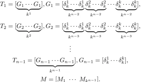
Lemma 3 Consider an n-stage NFSR with a feedback function f. Let M = [M1M2 · · · Mkn−1]be the structural matrix of NFSR which can be got the truth
table off, arranged in the reverse alphabet order, andL= [L1 L2 · · · Lkn−1]be
the state transition matrix. Then we have Colj(Li) =δ
(i−1)k+j
kn−1 Colj(Mi), where
L∈ Lkn×k, M∈ Lk×k, j= 1,2, . . . , k, i= 1,2, . . . , kn−1.
Proof. View the NFSR as a k-valued logic network. Then the NFSR can be expressed as the following logic network:
x1(t+ 1) =x2(t),
x2(t+ 1) =x3(t),
.. .
xn−1(t+ 1) =xn(t),
xn(t+ 1) =f(x1(t), x2(t), . . . , xn(t)),
wherexi∈ Dk, i= 1,2, . . . , n,andf :Dkn→ Dk.LetTi be the structure matrix
of xi(t+ 1) = xi+1(t), i ∈ 1,2, . . . , n−1, and M be the structure matrix of
xn(t+ 1) =f(x1(t), x2(t), . . . , xn(t)). Then it is easy to see that
T1= [G| {z }1· · ·G1
k1
], G1= [δk1· · ·δ
1
k
| {z }
kn−2
δk2· · ·δ2k
| {z }
kn−2
· · ·δkk· · ·δkk
| {z }
kn−2
],
T2= [G| {z }2· · ·G2
k2
], G2= [δk1· · ·δ
1
k
| {z }
kn−3
δk2· · ·δ2k
| {z }
kn−3
· · ·δkk· · ·δkk
| {z }
kn−3
],
.. .
Tn−1= [Gn−1· · ·Gn−1
| {z }
kn−1
], Gn−1= [δk1· · ·δ k k],
M = [M1 · · · Mkn−1].
Then (1) shows that the unique state transition matrixLsatisfyingL=T1∗T1∗
· · ·Tn−1∗M, where ”*” is the Khatri-Rao product. Straightforward computations
yield the columns ofLsatisfying
Colj(Li) =δ
(i−1)k+j
wherej = 1,2, . . . , k, i= 1,2, . . . , kn−1.
Theorem 4 Let the state transition matrix of NFSR beL=δkn[η1η2 · · · ηkn],
the structural matrix be M = δk[p1 p2 · · · pkn], and [s1 s2 · · · skn] be the
truth table of the feedback function f. Then ηi = (i (modkn−1)−1)k+pi =
i(mod kn−1)k−s
i.
Proof.We simplify the representation
Colj(Li) =δ
(i−1)k+j
kn−1 Colj(Mi),
wherej = 1,2, . . . , k, i= 1,2, . . . , kn−1.
Let (i−1)k+j=m, then straightforward computations show that
ηi= (i−1)k+pi,
ηi+kn−1 = (i−1)k+pi+kn−1,
ηi+2kn−1 = (i−1)k+pi+2kn−1,
.. .
ηi+(k−1)kn−1 = (i−1)k+pi+(k−1)kn−1.
(4)
wherei= 1,2, . . . , kn−1.
Thereforeηi= (i (mod kn−1)−1)k+pi, i= 1,2,· · ·, kn. Moreover, since si=
k−pi, we haveηi= (i (mod kn−1)−1)k+pi= (i (mod kn−1)−1)k−si,where
i= 1,2, . . . , kn.
4
Stability of Multi-valued Nonlinear Feedback Shift
Registers
In the beginning of this section, we first briefly review some existing basic defi-nitions and properties about the stability of NFSRs.
The state diagram of an n-stage, k-valued NFSR is a directed graph con-sisting of kn nodes and kn directed edges. Each node corresponds to a state of
the NFSR, and an edge from state X to state Y means that X is shifted to the state Y. X is called a predecessor of Y, and Y is called the successor of X. Every state of an NFSR has a unique successor, but may have no predeces-sor or a single predecespredeces-sor or two predecespredeces-sors. The state with two predecespredeces-sors is called a branch state, while the state without predecessors is called a start-ing state. A sequence of pdistinct states, X1,X2,· · · ,Xp, is called a cycle of
length p if X1 is the successor of Xp, and Xi+1 is a successor of Xi for any
i∈ {1,2,· · · , p−1}.Similarly, a sequence ofpdistinct states,X1,X2,· · · ,Xp is
called a transient of length p, if the following conditions are satisfied: (1) none of them lies on a cycle; (2)X1 is a starting state; (3) Xi+1 is a successor ofXi
for anyi∈ {1,2,· · · , p−1}; (4) the successor ofXp lies on a cycle.
We considerg= [g1g2 · · · gn],x= [x1x2 · · · xn]∈ Dkn,(1) can be expressed
as:
View the n-stage k-valued NSFR as a k-valued logic network, then it can be expressed as (5). For any positive integer N, let gN+1(X(t)) = g(gN(X(t))),
which indicates that the stateg(X(t)) is shiftedN+ 1 times fromX(t).
Definition 4 A state X(t) is called an equilibrium state of the logic network (5), if g(X(t)) = X(t). If the logic network (5) is a representation of an k -valued NFSR, then its equilibrium state is also called an equilibrium state of the NFSR.
Obviously, the logic network (5) haskpossible equilibrium states,i= [i i · · · i], i= 0,1,· · · , k−1. Without loss of generality, throughout this paper, we assume0 is an equilibrium state of the logic network representation (5) of an NFSR, or equivalently, the feedback function f of the NFSR satisfies f(0) = 0. For the equilibrium statei, through a coordinate transformation
¯
X(t) =X(t)⊕k−i,
the logic network (5) becomes
¯
X(t+ 1) =g( ¯X(t) +k−i) +k−i. (6)
It is easy to see that0is the equilibrium state of the logic network (6).
Definition 5 An n-stage NFSR is globally stable to the equilibrium state 0, if for any stateX(t), there exists a positive integerN such that the state transition function of its logic network representation (5) satisfies gN(X(t)) = 0, that is,
0is the unique equilibrium state and there are no cycles in the state diagram of the NFSR.
Definition 6 An n-stage NFSR is locally stable to the equilibrium state 0, if there exists some state X(t) ̸= 0 such that for some positive integer N
the state transition function of its Boolean network representation (1) satisfies gN(X(t)) =0.
Since ann-stage NFSR has an equivalent logic network representation in a linear system (2), accordingly, we give an equivalent definition of globally (locally) stable NFSR as follows.
Definition 7 An n-stage NFSR is globally stable to the equilibrium state 0, if for any statex(t), there exists a positive integerN such that the state transition matrixL of its logic network representation (2) satisfiesLNx(t) =δkknn.
Definition 8 An n-stage NFSR is locally stable to the equilibrium state 0, if there exists some statex(t)̸=δkn
kn such that for some positive integerN the state
transition matrixLof its logic network representation (2) satisfiesLNx(t) =δkn kn.
Definition 9 An NFSR is called a globally stable maximum transient NFSR if it is globally stable and has a single starting state.
Some properties of local stability are next given.
Theorem 5 An NFSR is locally stable if and only if the feedback function sat-isfies f(0,· · · ,0) = 0, and there are at least i ∈ {1,2,· · ·, k −1} such that
f(i,0,· · ·,0) = 0.
Proof.Necessity: Clearly, according to Definition 6,f(0,· · ·,0) = 0 is a neces-sary condition for a locally stable NFSR. For any NFSR whose feedback function
f satisfies f(0,· · · ,0) = 0,the state 0 has only two possible predecessors: itself and [i0 · · · 0], i∈ {1,2,· · ·, k−1}. If the NFSR is locally stable, then there ex-ists some stateX(t)̸=0such that for some integerN,gN(x(t)) = 0. Thus,0has a predecessor different to itself. Hence, here there are at leasti∈ {1,2,· · ·, k−1} such thatf(i,0,· · ·,0) = 0.
Sufficiency: f(0,· · ·,0) = 0 implies that 0 is an equilibrium state of the NFSR. If there are at least i ∈ {1,2,· · · , k−1} such that f(i,0,· · ·,0) = 0,
then [i0 · · · 0] is a predecessor of0. In other words, there exists a statex(t) = [i,0,· · · ,0] such thatg(x(t)) = 0, which implies that the NFSR is locally stable.
Theorem 6 Let L = δkn[η1 η2 . . . ηkn] be the state transition matrix of the
logic network representation (2) in a linear system of ann-stage NFSR. Then the NFSR is locally stable, thenηkn=kn and there are at leasti∈ {1,2,· · ·, k−1}
such that η(k−i)kn−1 =kn.
Proof.The result follows from (4) in Theorem 4 and Theorem 5.
Theorem 7 Let L = δkn[η1 η2 . . . ηkn] be the state transition matrix of the
logic network representation (2) in a linear system of an n-stage locally stable NFSR. Assume the initial state of system (2) be x0=δkrn, if
(1)colkn(L) =δk n
kn;
(2)there exists an integerl, such thatcolr(Ll) =δk
n
kn.
Proof.Clearly, according to Definition 8,f(0,· · ·,0) = 0 is a necessary condi-tion for a locally stable NFSR, i.e.,skn= 0, according to (4) in Theorem 4, we
have ηkn=kn, i.e.,colkn(L) =δk n
kn,
There exists an integerl, such thatcolr(Ll) =δk
n
kn.thusLlδkrn=δk n
kn.
This completes the proof.
Next, some properties of global stability are next given.
Theorem 8 If the NFSR is globally stable maximum transient, then there exists a uniquei∈ {1,2,· · · , k−1} such that f(i,0,· · · ,0) = 0.
Proof. If the NFSR is globally stable maximum transient, then other states have unique predecessor and successor, except the starting state and the state0. the state0has only two types of possible predecessors: itself and [i,0,· · · ,0], i∈
Theorem 9 LetL=δkn[η1η2 . . . ηkn]be the state transition matrix of the logic
network representation (2) in a linear system of ann-stage NFSR. If the NFSR is globally stable maximum transient, then there exists a uniquei∈ {1,2,· · · , k−1} such that ηkn=η(k−i)kn−1 = 0.
Proof.As the NFSR is globally stable maximum transient, then there exists a unique i ∈ {1,2,· · · , k−1} such that f(i,0,· · ·,0) = f(0,0,· · ·,0) = 0, thus
skn=s(k−i)kn−1= 0. The result follows from Theorem 4.
Theorem 10 LetLbe the state transition matrix of the logic network represen-tation (2) in a linear system of ann-stage NFSR. If the NFSR is globally stable, then there exists an integerN such that each columns of LN are equal toδkn
kn.
Proof.As the equilibrium state0∈ Dkn is uniquely corresponding to the state
δkknn ∈ ∆kn, that an n-stage NFSR is globally stale to the equilibrium state
0 is equivalent to that the n-stage NFSR is globally stable to the state δkknn.
Clearly, any state of an n-stage globally stable NFSR with one more starting states must be shifted fewer times to reach the equilibrium state0than then -stage globally stable maximum transient NFSR. For ann-stage globally stable maximum transient NFSR, the starting statex0=δkin, must shiftkn−1 times
to go through all other states and finally reaches the stateδkn
kn.(or equivalently,
the state0) and keeps staying at this state. Therefore,N=kn−1 is the largest
power such that each column ofLN is equal toδkn kn.
Theorem 11 Let L = δkn[η1 η2 . . . ηkn] be the state transition matrix of
the logic network representation in a linear system of an n-stage NFSR. Then,
δjkn, j∈ {1,2,· · · , kn}is a branch state if and only if there exist at least two
dif-ferent elementsa1, a2in the set{0,1,· · · , k−1}such thatηa1kn−1+i=ηa2kn−1+i=
j andi=⌈kj⌉.
Proof.(Sufficiency)ηa1kn−1+i =ηa2kn−1+i=j,thenLδa1kn−1+i=Lδa2kn−1+i=
δjkn, thusδkjn, j∈ {1,2,· · · , kn}is a branch state.
(Necessity) If δkjn is a branch state. According to Lemma 1, the state δ
j kn is
uniquely corresponding to the state X = [X1X2 · · · Xn]
T ∈ Dn
k satisfying
kn−1X
1+kn−2X2+· · ·+Xn = kn−j. The state X is a branch state, then
it has at least two possible predecessor: [k−1−a1, X1,· · · , Xn−1]T and [k−
1−a2, X1,· · · , Xn−1]T, wherea1, a2 ∈ {0,1,· · ·, k−1} anda1̸=a2.Since the
matrixLuniquely corresponds to the truth table of the feedback function that is arranged in the reverse alphabet order, accordingly we arrange allkn states
in Dn
k of the NFSR in the reverse decimal order as well. Thus, it is easy to
see that if we denote as Xa1kn−1+i = [k−1−a1, X1,· · ·, Xn−1]
T, and then
Xa2kn−1+i= [k−1−a2, X1,· · ·, Xn−1]
T. According to Lemma 1, we have
kn−a1kn−1+i= (k−1−a1)kn−1+X1kn−2+· · ·+Xn−1. (7)
According to (7) and (8), we have
kn−j=k(X1kn−2+X1kn−2+· · ·+Xn−1)+Xn=k(kn−1−i)+Xn =kn−ki+Xn.
It yieldski=j+Xn, SinceXn∈ {0,1,· · ·, k−1},we conclude thati=⌈kj⌉.
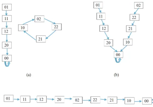
Fig. 2.The State Diagram of The Example
In the end of this section, an example is given to show the effectiveness of the results obtained in this paper.
ExampleConsider the following three 2-stage 3-valued NFSRs. The state0 is their equilibrium state.
Consider a nonlinear feedback shift register with a feedback function:
f1(x1, x2) =x1+x2+x21+ 2x 2 1x
2
2. (9)
Using the vector form, 0∼δ3
3,1∼δ32,0∼δ31, we obtain from (9):
f1(x1, x2) =δ3[1 0 0 0 2 2 2 1 0]x1x2=M1x1x2.
The state diagram in Fig.2 (a) shows it is locally stable. According to (4) in Theorem 4, we have:
x(t+ 1) =δ9[2 6 9 3 4 7 1 5 9]x(t) =L1x(t).
L21=δ9[6 7 9 9 3 1 2 4 9], L31=δ9[7 1 9 9 9 2 6 3 9], L41=δ9[1 2 9 9 9 6 7 9 9].
f(0,0) = 0, 0is a unique equilibrium state. According to Theorem 5, Theorem 6,f(2,0) =f(2,1) = 0,andη3=η9= 9.According Theorem 7, the initial state
Consider a nonlinear feedback shift register with a feedback function:
f2(x1, x2) =x1+x2+ 2x1x22+ 2x 2 1x
2
2. (10)
Using the vector form, 0∼δ33,1∼δ32,0∼δ31, we obtain from (10):
f2(x1, x2) =δ3[2 3 3 3 1 3 1 2 3]x1x2=M2x1x2.
The state diagram in Fig.2 (b) shows it is locally stable. According to (4) in Theorem 4, we have:
x(t+ 1) =δ9[2 6 9 3 4 9 1 5 9]x(t) =L2x(t).
L2
2=δ9[6 9 9 9 3 9 2 4 9], L32=δ9[9 9 9 9 9 9 6 3 9], L42=δ9[9 9 9 9 9 9 9 9 9].
δ9
9 is a branch state, according to Theorem 11, there exist at least two different
elements η3, η6 such thatη3 =η6 = 9. According Theorem 10, there exists an
integer N= 4 such that each columns of L42are equal toδ99.
Consider a nonlinear feedback shift register with a feedback function:
f3(x1, x2) = 2x1+x2+x21+x1x22+x 2 1x
2
2. (11)
Using the vector form, 0∼δ3
3,1∼δ32,0∼δ31, we obtain from (11):
f3(x1, x2) =δ3[2 3 1 3 1 3 1 2 3]x1x2=M3x1x2.
The state diagram in the last picture of Fig.2 shows it is globally stable maximum transient. According to (4) in Theorem 4, we have:
x(t+ 1) =δ9[2 6 7 3 4 9 1 5 9]x(t) =L3x(t).
L2
3=δ9[6 9 1 7 3 9 2 4 9], L33=δ9[9 9 2 1 7 9 6 3 9], L43=δ9[9 9 6 2 1 9 9 7 9], L23=
δ9[9 9 9 6 2 9 9 1 9], L33=δ9[9 9 9 9 6 9 9 2 9], L43=δ9[9 9 9 9 9 9 9 6 9], L43=
δ9[9 9 9 9 9 9 9 9 9].According Theorem 8, there exists a unique state [1 0] such
thatf(1,0) = 0.there exists an integer 8 such that each columns ofL83are equal toδ99.
Remark 1 In [25], we know the starting state of a globally stable maximum transient NFSR is [0 0 · · · 1] when k = 2. While k > 2, the starting state of a globally stable maximum transient NFSR is not unique. For example, when
k = 3, n = 2, we consider two nonlinear feedback shift registers with feedback functionsf(x1, x2) = 2x1+x2+x21+x1x22+x21x22 andf(x1, x2) = 2x1+x2+
2x21+2x1x22+x 2 1x
2
2respectively. They are both globally stable maximum transient,
but their starting states are [0 1]and[0 2]respectively.
5
Conclusion
matrices by considering it as a logical network via a semi-tensor product ap-proach. The new state transition matrix which can be simply computed from the truth table of its feedback function is easier to compute and is more ex-plicit. Then, based on the linearization theory of multi-valued NFSRs, globally (locally) stable multi-valued NFSRs were investigated. Some sufficient and neces-sary conditions were given. These results provide a method to construct globally or locally stable NFSRs, and are also helpful to analyze the state diagram of a NFSRs.
References
1. M. Hell, T. Johansson, and W. Meier, Grain-A Stream Cipher for Constrained Environments, eSTREAM, ECRYPT Stream Cipher Project, Report 2005/010, 2005.
2. S. Babbage and M. Dodd, The Stream CipherMICKEY (version 1), eSTREAM, ECRYPT Stream Cipher Project, Report 2005/015, 2005.
3. C. De Canni`ere and B. Preneel, Trivium Specifications, eSTREAM, ECRYPT Stream Cipher Project, Report 2005/030, 2005.
4. J. L. Massy, R. W. Liu, Application of Lyapnunovs direct method to the error-propagation effect in convolutional codes. IEEE Trans. Information Theory 10 (1964) 248-250.
5. J. Zhong and D. Lin, On maximum length nonlinear feedback shift registers us-ing a Boolean network approach, In: Proceedus-ings of the 33rd Chinese Control Conference, Nanjing, China, July 28-30, 2014, pp. 2502-2507.
6. C. Fontaine, Nonlinear feedback shift register, Encryclopedia of Cryptography and Security, pp. 846-848, 2011.
7. S. W. Golomb, Shift Register Sequences, Holden-Day, Laguna Hills, CA, USA, 1967.
8. J. Zhong and D. Lin, Stability of Nonlinear Feedback Shift Registers, Proceeding of the IEEE International Conference on Information and Automation , Hailar, China, July, 2014, in press.
9. S. Huang and I. Ingber, Shape-dependent control of cell growth, differentiation, and apotosis: switching between attractors in cell regulatory networks, Exper. Cell Res., vol. 261, no. 1, pp. 91-103, 2000.
10. M. Aldana, Boolean dynamics of networks with scale-free topology, Physica D, vol. 185, no.1, pp. 45-66, 2003.
11. D. Cheng, Disturbance decoupling of Boolean control networks, IEEE Trans. Au-tom. Control, vol. 56, no. 1, pp. 2-10, 2011.
12. D. Cheng, H. Qi, and Z. Li, Analysis and Control of Boolean Networks, London, U. K.: Springer-Verlag, 2011.
13. D. Laschov and M. Margaliot, A maximum principle for single-input Boolean control networks, IEEE Trans. Automatic Control, vol. 56, no. 4, pp. 913-917, 2011.
14. G. Hochma, M. Margaliot, E. Fornasini, and M. E. Valcher, Symbolic dynamics of Boolean control networks, Automatica, vol. 49, no. 8, pp. 2525-2530, 2013. 15. D. Cheng and H. Qi. Controllability and observability of Boolean control
net-works. Automatica, 45(7): 1659-1667, 2009.
17. Z. Li and D. Cheng. Algebraic approach to dynamics of multi-valued networks. Int. J. Bifurcat. Chaos, 20(3): 561- 582, 2010.
18. Z. Liu and Y. Wang. Disturbance decoupling of mix-valued logical networks via the semi-tensor product. Automatica, 48(8): 1839-1844, 2012.
19. D. Laschov and M. Margaliot. Controllability of Boolean control networks via the Perron-Frobenius theory. Automatica, 48(6): 1218-1223, 2012.
20. Y. Wang, C. Zhang and Z. Liu. A matrix approach to graph maximum stable set and coloring problems with application to multi-agent systems. Automatica, 48(7): 1227-1236, 2012.
21. D. Cheng, H. Qi, Z. Li, and J. B. Liu, Stability and stabilization of Boolean networks, Int. J. Robust and Nonlinear Control, vo. 21, no. 2, pp. 134-156, 2011. 22. F. Li and J. Sun, Stability and stabilization of multivalued logical network,
Non-linear Analysis: Real Word Applications, vol. 12, no. 6, pp. 3701-3712, 2011. 23. A. H. Roger and C. R. Johnson. Topics in Matrix Analysis. U.K.: Cambridge
University Press, 1991.
24. X. Zhang, Z. Yang, and C. Cao. Inequalities involving Khatri-Rao products of positive semi-definite matrices. Applied Mathematics E-notes 2: 117-124, 2002. 25. F. J. Mowler, Relations between Pn cycles and stable feedback shift registers,