and Reconstruction: A First Study
Changhai Ou, Chengju Zhou and Siew-Kei Lam
Hardware & Embedded Systems Lab, School of Computer Science and Engineering, Nanyang Technological University, Singapore.
[email protected],[email protected],[email protected]
Abstract. An important prerequisite for Side-channel Attack (SCA) is leakage sam-pling where the side-channel measurements (e.g. power traces) of the cryptographic device are collected for further analysis. However, as the operating frequency of cryptographic devices continues to increase due to advancing technology, leakage sampling will impose higher requirements on the sampling equipment. This paper undertakes the first study to show that effective leakage sampling can be achieved without relying on sophisticated equipments through Compressive Sensing (CS). In particular, CS can obtain low-dimensional samples from high-dimensional power traces by simply projecting the useful information onto the observation matrix. The leakage information can then be reconstructed in a workstation for further analysis. With this approach, the sampling rate to obtain the side-channel measurements is no longer limited by the operating frequency of the cryptographic device and Nyquist sampling theorem. Instead it depends on the sparsity of the leakage signal. Our study reveals that there is large amount of information redundancy in power traces obtained from the leaky device. As such, CS can employ a much lower sampling rate and yet obtain equivalent leakage sampling performance, which significantly lowers the requirement of sampling equipments. The feasibility of our approach is verified theoretically and through experiments.
Keywords: compressive sensing·matching pursuit·OMP·CoSaMP ·SP·GOMP
·side-channel attack
1
Introduction
Traditional side-channel leakage sampling conforms to the Nyquist theorem, i.e. the sampling rate of the equipment must be more than (or at least) twice the highest operating frequency of the cryptographic device in order for the original leakage to be reconstructed completely from the samples. In order to obtain more leakage details for Side-Channel Attacks (SCAs), the sampling rate is usually several times higher than the operating frequency of the leaky device. With advancing technology, the operating frequency of cryptographic devices is increasing rapidly. Micro-controllers and Field-Programmable Gate Arrays (FPGAs) today have a clock operating frequency of a few MHz, while mobile phones, laptops and desktop computers can run in the order of several GHz.
conform to the sampling rate that is dictated by the Nyquist theorem. In particular, using CS, the leakage sampling rate depends solely on the sparsity of the leakage signal, which is a predominant characteristic in the power traces obtained from the leaky device.
While there has been several works in SCA that have attempted to eliminate the information redundancy in power traces, these techniques only process power traces after leakage sampling to reduce the efforts of side-channel analysis. Contrary to our work, they do not lower the requirements on the sampling equipments. In the following subsection, we will discuss these existing works along with CS before describing the main contributions of our work.
1.1
Related Works
Points-Of-Interest (POI) selection in [DS16] and dimensionality reductions in [CDP15,
SNG+10,BHvW12] are two classical pre-processing techniques in SCA. The former finds
the locations of POIs by using side-channel distinguishers such as Differential Power Anal-ysis (DPA) [KJJ99] and Correlation Power Analysis (CPA) [BCO04], or leakage detection tools such as Welch’s t-test [DCE16],ρ-test [DS16] andχ2-test [MRSS18], while the latter
such as PCA [SNG+10] and LDA [SA08], considers the global features of high-dimensional
samples. Both techniques need to consider multiple power traces simultaneously. Discrete Wavelet Transform(DWT), Discrete Cosine Transform(DCT) and Fast Fourier Transform (FFT) [GHT05], transform power traces from time domain to sparse domain one at a time, but all the computations are carried out on the sampling equipments, which increases its workload and reduces the sampling rate.
To the best of our knowledge, Maximum Extraction and Integration in [MOP07] are two existing compressive sampling techniques that are used to eliminate information re-dundancy on power traces. The former maintains that the highest correlation occurs exactly at the position where the power consumption of each clock cycle reaches its max-imum, and it is therefore reasonable to choose these points as representative points for entire clock cycles. The latter integrates points in each clock cycle or within small time intervals. They are all applicable to situations where the sampling rate of the oscilloscope is much higher than the bandwidth of the leaky device. Re-sampling is then performed on the collected power traces. As such, these techniques incur resource wastage since the high sampling rate provides observers with leakage containing a large amount of redundancy, which is discarded during compression. This led to the problem stated in [Don06]: "why go to so much effort to acquire all the data when most of what we get will be thrown away? Can’t we just directly measure the part that won’t end up being thrown away?". The rest of this paper will address this problem for SCA.
Based on the theory of functional analysis and approximation [Kas91], Romberg, Tao and Donoho established the theory of Compressive Sensing (CS) [CR06,CRT06,Don06]. Combined with information theory, CS makes it possible to sample signals at a rate far below the Nyquist sampling theorem while enabling equivalent sampling performance. CS has been widely studied and applied to many fields such as image, voice and signals in general. The sampling rate of CS no longer depends on the highest frequency of the signals, but instead it is governed by the signal’s sparsity and Restricted Isometry Property (RIP) [CRT06]. As long as a signal is compressible or sparse in a certain transform domain, it can be projected from high-dimensional space into a low-dimensional space and retain the important information. Then, by solving an optimization problem, this signal can be reconstructed from a small number of projections with a high probability. In the context of SCA, sparsity provides a more intuitive and efficient representation of information in the power traces.
signifies that the low-dimensional transformed vector is sparse or approximately sparse when a high-dimensional leakage signal is projected onto a certain orthogonal transfor-mation basis. The aim is to find the features of signals in different functional spaces such as FFT, DWT, DCT and Bandelet [PM00], and provide a more concise representation. This is different from directly transforming the power traces into frequency domain, since the observer only needs to compute the inner product of the signal and the observation matrix, which requires very low computation. The purpose of the observation matrices such as Gauss, Bernoulli and Toeplitz [SYZ08] is to find a projection matrix that is not related to the sparse matrix, and they reflect the observation rules for leakage signals.
Fast and robust signal reconstruction algorithms are the most widely researched among the three aspects of CS. The algorithms can be divided into three categories according to the problem addressed: greedy algorithms for solving l0-norm, convex optimization
algorithms for solving l1-norm and the combination of these two kinds of algorithms.
Matching pursuit algorithms are typical examples of greedy algorithms, which aim to select one or more dimensions with the highest correlation with the current residual vector in each iteration, and approximate the original leakage signal and the new iteration error based on the current selected dimensions. Classical greedy algorithms include Matching Pursuits (MP) [MZ93], Orthogonal Matching Pursuit (OMP) [SM15], CoSaMP[NT10], GOMP [WKS12], TMP (Tree Matching Pursuit) [LD06] and ROMP [NV09], etc. Convex relaxation algorithms convert the non-convex optimization probleml0-norm to the convex
optimizationl1-norm. The representative algorithms include BP (Basis Pursuit) [CDS01],
GP (Gradient Projections) [HTWM10], IHT (Iterative Hard Threshold) [Mal09], etc. The convex optimization algorithms are more accurate than the greedy algorithms, but their computational complexity is higher. The combined or hybrid algorithms mainly consist of CP (Chaining Pursuit) [GSTV06]. It is worth mentioning that even though there are many existing reconstruction algorithms, there are still a lot of problems in their convergence and robustness. Nevertheless, the existing theories and prior work are sufficient for CS to be applied in side-channel leakage sampling.
1.2
Our Contributions
The increasing operating frequency of cryptographic devices impose high requirements on the sampling equipments, bring new challenges to the storage and processing of power traces for SCA. In this paper, we focus on addressing these challenges which pertain to leakage sampling for SCA. While this problem has not been adequately discussed in the literature, we believe it is of high importance as we are able to show that the high operating frequency of advanced cryptographic devices is not a barrier to leakage sampling in the absence of powerful sampling equipments.
Specifically, we introduce a novel use of Compressive Sensing (CS), a new and highly-efficient compressive sampling technology for side-channel leakage sampling. CS performs compression and sampling simultaneously by projecting the high-dimensional signals on-to a low-dimensional space on-to obtain the discrete leakage samples. This enables the high-dimensional signal to be reconstructed without distortion. Compared with classi-cal sampling, CS uses a far lower sampling rate to achieve the same performance. The feasibility of our approach is verified by theory and experiments in this paper.
Windows 7 operation system, even allow the development of independent sampling soft-ware. Researchers have also developed the sampling software on various platforms. For example, Inspector developed by Riscure, enables the leakage to be collected and stored on laptop computers and other advanced processors. CS can also be efficiently imple-mented on these platforms by integrating a small program to solve the inner product of observation matrix (see Section4) and leakage sample vector.
1.3
Organization
The rest of this paper is organized as follows. Principles of classical compressive sam-pling and CS are introduced in Section 2. The first two main parts of CS, leakage sparse representation and observation, are described in Sections 3∼4. Section 5 uses classical greedy algorithms such as OMP, CoSaMP, SP and GOMP as examples to introduce the principle of signal reconstruction. The corresponding reconstruction performance evalua-tion criteria are also provided in this secevalua-tion. Observers can find good sparse domain and observation matrix through experiments, optimize the sparse coefficients and compression ratio, and implement CS with a much lower sampling rate than those required by existing sampling equipments or sampling software on computers. In Sections 6 and 7, we describe the experiments on an AT89S52 micro-controller and measurements from DPA contest v1.1 [dpa] to demonstrate the efficiency of the approach. Finally, Section 8 concludes this paper.
2
Preliminaries
2.1
Classical Compressive Sampling
Sampling and compression are carried out separately in traditional compressive sampling. The sampling rate must satisfy Nyquist theorem, which states that the bandwidth of sampling equipment must be at least twice the maximum frequency of the cryptographic device. Moreover, the sampling is uniform, and the number of samples collected in any fixed interval is the same. It is noteworthy that the sampling rate is usually much higher than the bandwidth of cryptographic devices in practice. As such, the power traces contain a large amount of information redundancy, which can be removed during compression to lower the complexity of side-channel attacks and evaluations. Mangard et al. stated that the peaks of the damped oscillation carried all the information that was necessary to perform a power analysis attack. Two classic compression techniques named Maximum Extraction and Integration were given [MOP07]. The reconstruction of the original power traces from compressed ones is usually not considered in SCA since attacks can be directly performed on the compressed low-dimensional power traces.
Dimensionality reduction methods such as PCA [SNG+10, BHvW12], LDA [SA08],
KDA [CDP16] and manifold learning [OSW+17], obtain the low-dimensional samples by
necessary, which requires significant effort.
2.2
Compressive Sensing
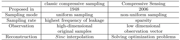
The principle of CS maintains that as long as the signal is sparse or sparse in a trans-form domain, and its projection vectors can be obtained from observation matrix, then it can be reconstructed nondestructively by optimization methods. Unlike the classical compressive sampling, wherein the sampling and compression are performed separately, CS compresses a power trace while sampling it and aims to use the least coefficients to represent the compressed signal. Compared with traditional compressive sampling, the sampling rate in CS theory no longer depends on the bandwidth of signal, but on it-s it-sparit-sity (it-see Table 1). The it-sparit-ser the it-signal in a tranit-sformation domain, the fewer non-zero coefficients it possesses. These coefficients represent the smallest sampling band-width needed to reconstruct the original high-dimensional signals. As such, to achieve the same sampling performance, CS only requires a much lower sampling rate compared to traditional compressive sampling.
Table 1: Difference between classic compressive sampling and CS.
classic compressive sampling Compressive Sensing
Proposed in 1948 2006
Sampling mode uniform sampling non-uniform sampling
Sampling rate highest frequency of leakage sparsity
Observation high-dimensional low dimensional
original samples observation vector
Reconstruction Sincinterpolation Solving optimization problems
Moreover, classical compression samples uniformly, while CS does not. The low-dimensional samples are obtained by computing the inner product between the signal and the observation matrix. Since each measured value takes the same information, this makes the measurement robust. Finally, Nyquist sampling theorem uses Sinc interpola-tion (i.e. Whittaker-Shannon interpolainterpola-tion) to reconstruct the original leakage, which is a linear operation with limited computation. CS uses nonlinear programming methods to recover leaky signals, and the corresponding complexity is high. Fortunately, most of the computation is eventually transferred from the sampling devices to computers, which notably reduces the workload of the sampling devices.
0 n
(a) original signal
0 n
(b) sparse representation
0 m
(c) observation
0 n
(d) signal reconstruction
→
→
→
Figure 1: General procedure of CS.
The complete CS flow is shown in Fig. 1. Firstly, them sparse coefficients of then -dimensional original signals are obtained by sparse transformation (m≪nin Fig. 1(b)).
original signal is projected onto a sparse domain to achieve low-dimensional samples. The sampling device outputs these samples as sampling results. Finally, the original signal is reconstructed by solving an optimization algorithm (Fig. 1(d)). These operations correspond to the three aspects of CS theory introduced in Section1.1: signal sparse rep-resentation, observation matrix design, and signal reconstruction, which will be discussed in detail in Sections III∼V.
3
Leakage Sparse Representation
3.1
Sparse Decomposition
The purpose of sparse decomposition in SCA is to use as few sparse vectors as possible to represent the original leakage. If a leakage signalx= [x0, x1, . . . , xn−1]∈Rn×1can be
represented by linear combinations of normal orthogonal bases Ψ = [ψ0, ψ1, . . . , ψn−1]∈
Rn×n, then
xcan be represented as:
x= ΨΘ =
n−1
X
i=0
ψiθi. (1)
If the number of non-zero coefficients k in Θ is much smaller than n, then x is
s-parse or compressible on the orthogonal basis Ψ. In other words, Θ is ss-parse. Θ = [θ0, θ1, . . . , θn−1]T ∈Rn×1is the sparse coefficients, and also the sparse representation of
xon Ψ. Ψ here is the sparse base or sparse domain.
3.2
Determination Conditions
The precondition of CS is that the leakage signal isk-sparse, but most of the natural signals are not sparse. If the absolute values of the coefficients in Θ exponentially attenuate after being sorted in descending order, the observer obtains
θ
′ 0
≥
θ
′ 1
≥ · · · ≥ θ
′ n−1
. For any
p∈(0,+∞), if there exists
θ
′ i
≤
R
p
√n, (2)
then the signal is compressible or nearly sparse. Herei∈(0, n−1). Parameterpcontrols the speed of exponential attenuation. The larger it is, the faster the attenuation, and the sparser the signal x is on Ψ. Therefore, the criterion to evaluate the performance
of a set of sparse bases is to measure the attenuation tendency of the sparse coefficients. However, many signals are not strictly sparse but approximately sparse, which can still be decomposed sparsely.
Candes and Tao indicated in [CT06] that the signals with Θ exponential attenuation could be reconstructed by CS theory, and the upper bound of reconstruction error satisfies:
eo=kx−xˆk2≤Cp·R·
k
logn
−r
. (3)
Here r= 1/p−1/2, 0< p <1,R >0,Cp is constant which only depends onpand k·k2
is thel2-norm.
3.3
Sparse Domains
longer preserve features of time domain. DCT focuses on the low frequencies of power traces as critical information. DWT can better analyze the time-domain characteristics of signals and more sparsely represent the information of signals. If a suitable base is selected, the coefficients are easier to deal with than the original leakage signal.
We only consider DCT in this paper. There are 8 transform forms for one-dimensional DCT, of which the second one is the most commonly used. Let ndenote the number of samples on original leakage signal, then theu-th coefficient after transformation is
F(u) =c(u)
n−1
X
i=0
x(i) cos
u(2i+ 1)
2n
. (4)
x(i) is the i-th time point of original leakage signal andc(u) is a coefficient satisfying
c(u) =
q
1
n, u= 0
q
2
n, u= 1,2,· · ·, n−1
(5)
It can be regarded as a compensation coefficient, which makes the DCT transformation matrix an orthogonal matrix. For side-channel leakage,c(0) ofF(0) is the DC (Direct-Current) component and other coefficients are AC (Alternating (Direct-Current) components. The complexity of DCT is O n2
. In fact, the target of reconstruction algorithms is to reconstruct the DCT coefficients. Finally, the Inverse Discrete Cosine Transform (IDCT):
x(i) =
r
2
n
n−1
X
u=0
c(u)F(u) cos
u(2i+ 1)π
2n
(6)
is performed to reconstruct the original leakage.
4
Observation
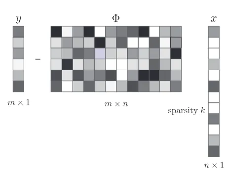
The sampling process of CS is very simple, and most of the computations lie mainly in the leakage signal reconstruction. This reduces the workload of sampling devices and facilitates the fast sampling of CS. If the leakage signal x ∈ Rn×1 is sparse, it can be
projected onto the observation matrix Φ = [φ0, φ1, . . . , φm−1]∈Rm×n:
y= Φx, (7)
and obtains the low-dimensional observation vector (as shown in Fig. 2). Otherwise, the observer must project it onto orthogonal bases to make it sparse. The observation matrix Φ is independent of the sparse basis Ψ. Herey= [y0, y1, . . . , ym−1]∈Rm×1is the
observation vector (i.e. sampling results of sampling equipment). y = ΛΘ (Λ = ΦΨ =
[γ0, γ1, . . . , γn−1]) is defined as the sensing matrix. The principle ofy= Φxandy= ΛΘ
is similar, since we can make
Θ = ΨT
x (8)
and get Φ′ = ΦΨT. The observation
y = Φ
′
x. Matrices Ψ and Φ can be employed
universally in a cryptographic implementation, and hence we only need to set them once. Since the size m of y is much smaller than the size n of x, y = ΛΘ is an
under-determined system of equation. This is equivalent toxbeing compressed, and the amount
m×n
Φ
m×1
n×1
x
y
sparsityk
=
Figure 2: Low-dimensional observation from high-dimensional leakage signalx.
4.1
Constraint Conditions
Observers need to construct an observation matrix in CS theory, which plays an important role in the acquisition of observation vectors and signal reconstruction. It requires that thekmeasured values do not destroy the information of the original leakage signal when it is converted from x to y, thus ensuring accurate signal reconstruction. This should
satisfy Restricted Isometry Property (RIP) and Incoherence Property [CW08,DH01].
Restricted Isometry Property: A matrix Ψ satisfies RIP of order k (i.e. the leakage signal is k-sparse) if there exists aδ ∈ (0,1) that makes Λ satisfy the following inequality:
1−δ≤ kΛΘk2
kΘk2 ≤1 +δ. (9)
This ensures that signals can be transformed from one domain to another without diver-gence. δis the Restricted Isometry Constant (RIC) [CRT06], which is the minimum value satisfying Eq. 9.
Incoherence property: The coherence within the observation matrix Φ is the maximum absolute value of the normalized inner products, i.e.
µ(Φ) = max
1≤i,j≤n,i6=j
|hφi, φji|
kφik2· kφjk2
. (10)
Hereh·,·idenotes dot product of two vectors. The smaller theµ, the weaker the coherence of any two atoms (i.e. columns) in Φ. The coherence coefficients of orthogonal matrices are 0.
The coherence between the observation matrix Φ and sparse transformation base Ψ can refer to the coherence between two atoms of a single matrix. Incoherence here means that the row vectorsφi of Φ cannot be represented linearly by the column vectors in Ψ.
The coherence of Φ and Ψ can be defined as:
µ(Φ,Ψ) =√n· max
1≤i,j≤n{|hφi, ψji|} ∈
0,√n
. (11)
4.2
Observation Matrices
It is difficult to directly design an observation matrix satisfying the RIP condition. Most of the current observation matrices are random Gaussian matrices, wherein each element satisfies the normal distribution with mean 0 and variance m1:
φ(i, j)∼ N
0, 1 m
. (12)
Since random matrices are not related to any matrix, they can satisfy RIP conditions with high probability if m ≥ c·k·log2 nk
[Don06]. Here c is a small constant. An-other observation matrix is random Bernoulli matrix, in which elements follow Bernoulli distribution:
φ(i, j) = √1m
1, pr= 12
−1, pr= 12
(13)
or
φ(i, j) =
r
3
m
1, pr=16
0, pr=23
−1, pr=16
(14)
Here pr denotes the probability of the element. Baraniuk et al. in [RMRM08] proved
that Bernoulli matrix was strongly random, it could satisfy RIP condition with great probability if the number of observationsm≥c·k·log2 nk
. Besides Gauss and Bernoulli, a large number of observation matrices have also been proposed, which will not be discussed in this paper.
5
Leakage Reconstruction
Signal reconstruction algorithms in CS aim to use the low-dimensional observation vector
y to recover the high-dimensional original leakage signalx. As proved in [GN03,Tro04],
if the sparse coefficients in Θ satisfy
kΘkl0 <
1 2
1 + 1
µ{Φ}
, (15)
the low-dimensional observation is achieved by solving the optimization problem:
arg minkΘkl0, s.t.y= ΛΘ. (16)
kΘkl0 is the number of non-zero elements in Θ. In this case, Θ has a unique solution,
which is equivalent to that the minimum number of linear correlation atoms in the given matrix Φ is greater than 2k. Thus, the sparse coefficient Θ is obtained and the side-channel leakagexis recovered by Eq. 1. The greedy algorithms aim to solve thel0-norm.
Sincem≪n,y= ΛΘ has multiple solutions, this is NP-hard. If a reconstruction errorǫ
is allowed, this model becomes
arg minkΘkl0, s.t. ky−ΛΘk< ǫ. (17)
5.1
Optimization
Since Θ is sparse, the number of unknowns in y= ΛΘ is greatly reduced, which makes
signal reconstruction possible. The problem described in Eq. 17 can be solved by the suboptimal solution ofl0-norm:
arg minkΘkl1, s.t.y= ΛΘ (18)
if θ satisfies certain conditions [CDS01]. The typical solutions of l1-norm are convex
optimization algorithms. Thelp-norm of vectorx= [x0, x1, . . . , xn−1]T is defined as
kxkl
p =
n−1
X
i=0
|xi|p
! 1 p
. (19)
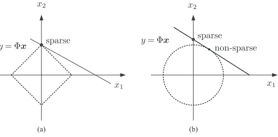
Taking two-dimensional real space R2 as an example, l
1-normkxkl1 =|x1|+|x2|
repre-sents the closed area surrounded by four lines shown in Fig. 3(a), and l2-norm kxkl2 =
q
|x1|2+|x2|2 represents a circle (as shown in Fig. 3(b)). They are hyper-prism and
hyper-sphere in high-dimensional spaceRn. Only if the optimal solution of
y= Φxfalls
onto the coordinate axis can the sparsity be guaranteed. In fact, if l1-norm andl2-norm
fall onto the coordinate axis, their solutions are equivalent to the ones ofl0-norm.
RULJLQDOVLJQDO VSDUVH
QSFTFOUBUJPO
REVHUYDWLRQ UHFRQVWUXFWHG
VLJQDO
(a) (E)
RULJLQDOVLJQDO
VSDUVHVLJQDO
REVHUYDWLRQ
UHFRYHUHG UHFRYHUHGVLJQDO
y=Φx
y=Φx sparse non-sparse
x1
sparse
x1 x2
x2
Figure 3: The geometric meaning of the optimal solutions ofl1-norm (a) andl2-norm (b)
in two-dimensional space.
From the perspective of information theory, the information cannot be infinite com-pressed. The number of observations (i.e. the number of measurements) m determines the compression ratio m
n. For a leakage signal with lengthnand sparsityk on a sparse
base, the lower bound of the number of observationsmrequired by CS is:
m≥c·µ2(Φ,Ψ)
·k·log2n. (20)
It is noteworthy that the above solutions all require the observer to solve constraint problems, which can be transformed into solving unconstrained problem [CT06]:
arg minkΘkl1+ηky−ΛΘk2. (21)
η is a balance factor, which is used to balance reconstruction error and sparsity.
5.2
Greedy Algorithms
in CS. Greedy algorithms are the earliest and the most widely used signal reconstruction algorithms in CS. The main idea of these algorithms is to select one or more atoms (i.e. columns) having the greatest correlation with the current residual vectorr in each iteration, and obtain the current optimal solution to approximate the original leakage signal and the new iteration error according to the currently selected atoms. Matching Pursuits (MP) [MZ93] and Orthogonal Matching Pursuit (OMP) (improved from MP) [SM15] are two widely used greedy algorithms in CS. MP selects the atom γt−1 with
highest matching degree between matrix Λ and current signal residualrt−1:
γt−1= arg max γj
|hrt−1, γji|. (22)
Here t−1 is the current number of repetitions (i.e. the current number of observations). The residual is then decomposed as
rt−1= max|hrt−1, γji|+rt (23)
after each iteration. Almost all of the matching pursuit algorithms such as CoSaMP[NT10], GOMP [WKS12], StOMP[DTDS12] and ROMP [NV09], are improved from OMP. These algorithms preserve the atom selection strategy of MP.
OMP [SM15] is the most commonly used algorithm in CS (see Algorithm 1). The atom in the sensing matrix Λ having greatest correlation with the current residualrt−1
is selected as a new candidate atom (Step 3). It is added to the atom matrix Λtand its
corresponding index λt is added to the support set A (Step 4). For a k-sparse leakage
signalx, onlyknon-zero coefficients are involved in the operation when the sensing matrix
Λ is used. These atoms are stored in matrix Λ according to the observation rules used during the iteration. OMP is then updated by subtracting its projection on the orthogonal space of the selected atom matrix from the observation vectoryuntil the iterationt≤k
is satisfied (Steps 5 and 6). Since the residual r is orthogonal to the selected atoms, an atom in Λ will not be selected twice, thus guaranteeing the convergence of the algorithm. Moreover, orthogonalization guarantees the local optimal solution in each iteration, but does not guarantees that the sum of the local optimal solutions is the global optimal solution.
Algorithm 1:Orthogonal Matching Pursuit (OMP).
Input: sensing matrix Λ = ΦΨ, sparse base Ψ, support matrixA, observationy
and sparsityk.
Output: estimated parameters ˆΘ and residualr.
1 Initialization: r0=y,A0=∅, Λ0=∅ and the number of iterationt= 1; 2 whilet≤k do
3 λt= arg max
j|hrt−1, γji|;
4 find indexAt=At−1∪ {λt},Λt= Λt−1∪ {γλ
t};
5 Θˆt= arg minˆ Θt
y−ΛtΘˆt
2 ; 6 update residualrt=y−ΛtΘˆt; 7 t=t+ 1 ;
8 end
9 recover signal ˆx= Ψ ˆΘ ;
OMP uses least square method to solve the minimum ˆΘt(see Step 5 in Algorithm 1).
Sincey= ΛΘ, solvingf(Θ) =ky−ΛtΘtk2is equivalent to solving:
The function f(Θ) has an extreme value at ∂f∂(Θ)Θ = 0, i.e. ∂f∂(Θ)Θ =−2ΛT
t (y−ΛtΘt).
We get ΛT
ty= ΛTtΛtΘt, Step 5 can be simplified by solving
Θt= ΛTtΛt
−1
ΛTty. (25)
Here ΛT
t is the transformation matrix of Λt. The complexity of OMP isO(k·m·n). The
advantage of OMP is its fast convergence and high accuracy under the precondition that
k is known. However, if the sparsityk is unknown and the estimation is too small, then the absolute erroreois too large, OMP falls into endless iterations or results in very low
percentage recovered. Moreover, it will incur a large amount of computation and lower the quality of reconstructed signals if the sparsitykis estimated to be too large.
As we mentioned earlier, almost all of matching pursuit algorithms are improved from OMP. An obvious disadvantage of OMP algorithm is that only one atom is selected in each iteration. With the number of observations increase, the runtime increases rapidly. This can be solved by selecting multiple atoms from the observation matrix Φ or sensing matrix Λ each time. In this case, SWOMP (Stagewise Weak OMP) [BD09] which is improved from StOMP (Stagewise OMP) [DTDS12], selects all the atoms larger than a preset threshold for subsequent calculations. The difference is that the threshold of StOMP comes from residuals, while the threshold of SWOMP comes from experiential setting. In general, the threshold of SWOMP is the maximum coefficient multiplied by a parameter between 0 and 1, with a default value 0.5. The complexity of StOMP and SWOMP is O(m·n). GOMP [WKS12] requires to set a parameter s, which denotes the number of atoms selected in each repetition (the default value is k
4). In order to
reduce parameter settings, we chose GOMP to represent these improved algorithms in our experiments.
Another disadvantage of OMP algorithm is that once an atom is in the candidate set, it will never be deleted. StOMP and SWOMP also have this drawback. To improve this shortcoming, two algorithms CoSaMP (Compressive Sampling Matching Pursuit) [NT10,NV10] and SP (Subspace Pursuit) [DM09], which rely on backtracking is employed. Specifically, as the algorithm iterates, the atoms in Λ are recalculated and the non-optimal atoms are deleted. Specifically, CoSaMP [NT10,NV10] selects 2·katoms most relevant to the residual in Steps 3 and 4 of Algorithm 1, and thekatoms with the largest absolute values in ˆΘ are selected for the next iteration in Step 5. It guarantees that there will be no more than 3·katoms in Λ, 2·k atoms inAand at mostk atoms are removed in each repetition. Compared with CoSaMP, SP [DM09] only selects katoms most relevant to the residual in Steps 3 and 4, it guarantees that there should be no more than 2·k
atoms in Λ and 2·katoms in support vectorA, and at mostkatoms are removed in each repetition. The complexity of CoSaMP and SP isO(m·n) andO(log (k)·m·n).
5.3
Performance Criteria
There are many criteria to evaluate the performance of signal reconstruction algorithms, such as reconstruction time, reconstruction residual (also called absolute error, see Eq. 3), relative error and signal-to-noise ratio (SNR). They reflect the reconstruction performance of the algorithm from different aspects.
Relative Error: Referring to the absolute erroreo=kx−xˆk2between the original
leakage signal xand reconstructed signal ˆx given in Eq. 3, the relative error is defined
as:
er=k
x−xˆk2
kxˆk2 . (26)
consump-tion component to noise component in side-channel attacks [MOP07]. It is defined as:
SNR = 20×lg
kxk2 kx−xˆk2
(27)
in CS, of which the molecule represents the variance of the signal. The denominator represents the absolute error of the original signal and the reconstructed signal.
Matching Degree: The matching degreeαof the original signal and the recovered signal is defined as
α= 1−|kxˆk2− kxk2|
|kxˆk2+kxk2|. (28)
It is a positive number with a value between 0 and 1. The smaller the reconstruction error
e0 =kx−xˆk2, the greater the matching degree, the closer to 1 the αis, and the better
the reconstruction performance.
Percentage Recovered: The percentage recovered Pr in [TG07] depends on the
absolute erroreo =kx−xˆk2 of reconstruction. If it is smaller than the pre-determined
threshold, then the reconstruction is successful. Therefore, its calculation is similar to the Success Rate (SR) [SMY09] in side-channel analysis, and its value is the ratio of the number of successful reconstructions to the total number of repetitions in experiments. The setting of threshold eo can be determined according to the required reconstruction
accuracy. If the reconstructed power traces are only used for attacks, it can be set ap-propriately large. However, leakage evaluations require high reconstruction accuracy, so it should be set small.
6
Experiment Results On AT89S52 Micro-controller
6.1
Experimental Setups
Our first experiment is performed on anAT89S52 micro-controller, with a clock operating frequency of 12 MHz. The shortest instructions take 12 clock cycles to execute. We use a Tektronix DPO 7254 oscilloscope to capture leakage of the look-up table instruction "MOVC A,@A+DPTR", which takes 24 clock cycles. The oscilloscope has a sampling rate of up to 40 GHz, but it does not have the function to automatically collect and store waveform. We obtain the waveform acquisition plug-in from the Tektronix company, but the speed is very slow. We cannot even store the leakage samples of the AES encryption algorithm promptly under 500 MHz sampling rate. So, we add about 0.5 second of empty-loop instructions before look-up table operation. Finally, we acquire 20000 power traces, each of them includes 5000 samples. The rest of our experiments are performed on a
HP desktop computer with 6 Inter(R) Xeon(R) E5-1650 v2 CPUs, 16 GB RAM and a Windows 10 operating system. It’s clock frequency is 3.5 GHz. Since the power traces are affected by noise, they fluctuate significantly. We use a moving average filter with a 5-hour span to remove the noise. A random observation matrix for four algorithms is generated for each repetition.
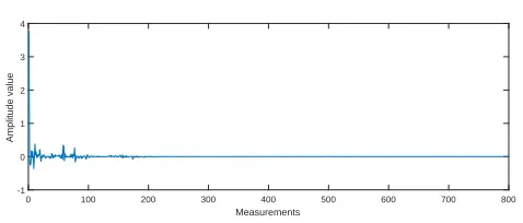
In order to observe and compare the performance of the algorithms OMP, CoSaMP, BP and GOMP, we use the 1801th∼2600thsamples to perform our CS using MATLAB
0 100 200 300 400 500 600 700 800 Measurements
-1 0 1 2 3 4
Amplitude value
Figure 4: DCT coefficients of a power trace leaks fromAT89S52 micro-controller.
6.2
Threshold Selection
The original power tracexcan be projected onto the observation matrix Φ if it satisfies
RIP, and reconstructed by using at least m ≥k·log2 nk
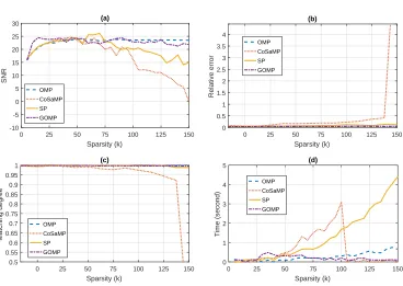
observations. The minimum number of observationsmcan be quickly obtained if the sparsitykis known. Otherwise, we need to test it. In order to optimize the reconstruction performance, it is necessary to adjust m appropriately. We use OMP, CoSaMP, SP and GOMP to perform our experi-ments and setmto 400 to test the sparsity, which ranges from 5 to 200, with step width 5. SNR, relative error, matching degreeαand their runtime under different sparsity are shown in Fig. 5. The reconstruction performance is compared considering only one power trace. The SNR of OMP, CoSaMP and SP increases rapidly and reaches the highest at
k < 80. SP and GOMP fluctuate significantly atk > 100. GOMP is the highest when
k <75, which indicates that its power trace reconstruction requires the smallest number of observations. SNR and matching degree of CoSaMP decrease rapidly whenk >125, the relative error of it is also much larger than other algorithms. Ifmis set to 320, the SNR of 4 algorithms reaches the highest at k <45, and SP fluctuates significantly atk >60. This also indicates that we may get very different results under different observations.
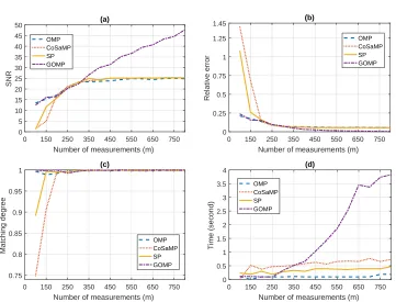
CoSaMP is the most time-consuming algorithm followed by SP (see Fig. 5(d)). It decreases rapidly to about 0 when k > 135, the observer should guarantee that there should be 3·katoms in Λ, which indicates that very largekwill affect its performance. The time consumption of OMP and GOMP only change a little under different sparsity. Through comprehensive analysis, reasonable k should be between 50 and 125, which is further set to 50 in the next experiments (if m = 320, k is then set to from 45 to 60). The experimental results of m from 100 to 800 are shown in Fig. 6. The SNR of the four algorithms continues to improve before the number of measurements m reach 320 (i.e. m≥k·log2 nk
is satisfied). OMP, CoSaMP and SP achieve optimal performance when m >300 (SNR is about 25). This indicates thatklimits the further improvement of their performance. However, the performance of GOMP is still improving and becomes the best when m > 300. The final SNR of GOMP is about 48. This is also reflected in Fig. 6(b) where the relative errors of OMP, CoSaMP and SP decrease to the lowest (about 0.055) whenm >300, while the relative error of GOMP continues to decline and finally reaches about 0.004. This also fully illustrates the superiority of GOMP.
0 25 50 75 100 125 150 175 200 Sparsity (k)
0 5 10 15 20 25 30 35
SNR
(a)
OMP CoSaMP SP GOMP
0 25 50 75 100 125 150 175 200 Sparsity (k)
0 1 2 3 4 5 6
Relative error
(b)
OMP CoSaMP SP GOMP
0 25 50 75 100 125 150 175 200 Sparsity (k)
0.5 0.6 0.7 0.8 0.9 1
Matching degree
(c)
OMP CoSaMP SP GOMP
0 25 50 75 100 125 150 175 200 Sparsity (k)
0 2 4 6 8 10 12
Time (second)
(d)
OMP CoSaMP SP GOMP
Figure 5: SNR (a), relative error (b), matching degree (c) and time consumption (d) of OMP, CoSaMP, SP and GOMP under different sparsity.
6.3
Performance Comparison
We randomly select a power trace. In fact, the reconstruction performance of power traces is almost the same under the same observation matrix. The algorithms OMP, CoSaMP, BP and GOMP can reconstruct power traces well whenk= 50 andm= 320 (as shown in Table 2 and Fig. 7). The blue line and red line represent the original and the reconstructed power traces. They overlap in most regions, when the matching degree is greater than 0.9950. This shows that only 320 samples need to be collected to reconstruct the leakage of 800 samples under CS. If we collect longer traces, the compression performance is even better. GOMP performs best, since the relative error er is smallest, of which the
corresponding SNR is also the largest. This also verifies the conclusion that SNR of GOMP is the highest whenk= 50 in Fig. 5. Althougher of OMP is larger than that of GOMP,
the matching degree of it is better. This indicates that partial overlap has an important impact on the overall performance evaluation. Therefore, we need to integrate a number of criteria when comparing the performance of power trace reconstruction algorithms.
Table 2: Leakage reconstruction performance of OMP, CoSaMP, SP and GOMP on
AT89S52 micro-controller.
algorithms er SNR α time (second)
OMP 0.0647 23.7766 0.9993 0.017782
CoSaMP 0.0573 24.8361 0.9971 0.092189
SP 0.0607 24.3335 0.9958 0.044551
GOMP 0.0538 25.3873 0.9992 0.055530
The reconstruction erroreoof OMP, CoSaMP, SP and GOMP in Fig. 7 is about 0.40.
0 150 250 350 450 550 650 750 Number of measurements (m) 0 5 10 15 20 25 30 35 40 45 50 SNR (a) OMP CoSaMP SP GOMP
0 150 250 350 450 550 650 750 Number of measurements (m) 0 0.25 0.5 0.75 1 1.25 1.45 Relative error (b) OMP CoSaMP SP GOMP
0 150 250 350 450 550 650 750 Number of measurements (m) 0.75 0.8 0.85 0.9 0.95 1 Matching degree (c) OMP CoSaMP SP GOMP
0 150 250 350 450 550 650 750 Number of measurements (m) 0 0.5 1 1.5 2 2.5 3 3.5 4 Time (second) (d) OMP CoSaMP SP GOMP
Figure 6: SNR (a), relative error (b), matching degree (c) and time consumption (d) of OMP, CoSaMP, SP and GOMP under different numbers of measurements.
0 200 400 600 800 Time samples 0 0.05 0.1 0.15 0.2 0.25 Power consumption (a) OMP
0 200 400 600 800 Time samples 0 0.05 0.1 0.15 0.2 0.25 Power consumption (b) CoSaMP
0 200 400 600 800 Time samples 0 0.05 0.1 0.15 0.2 0.25 Power consumption (c) SP
0 200 400 600 800 Time samples 0 0.05 0.1 0.15 0.2 0.25 Power consumption (d) GOMP
Figure 7: Leakage reconstruction using OMP, CoSaMP, SP and GOMP (the original power trace (blue) and reconstructed power trace (red)).
results are given in Fig. 8. Let Pr denote the percentage recovered in the rest of this
paper. We randomly select signals from a set of 20000 power traces for 400 repetitions in our experiments. The evaluation in Fig. 8(a) and Fig. 8(b) takes 5678.401890 and 5667.954980 seconds, respectively.
160 190 220 250 280 310 340 370 400 Number of measurements(M)
0 0.1 0.2 0.3 0.4 0.5 0.6 0.7 0.8 0.9 1
Percentage recovered
(b)
OMP CoSaMP SP GOMP
0 15 30 45 60 75 90 105 120 135 150 160 Sparsity level(K)
0 0.1 0.2 0.3 0.4 0.5 0.6 0.7 0.8 0.9 1
Percentage recovered
(a)
OMP CoSaMP SP GOMP
Figure 8: Percentage recovered under different sparsity levels (a) and different numbers of observations (b).
The performance of OMP, CoSaMP, SP and GOMP are very different whenk varies from 5 to 160 (m= 320), where it first becomes better and then worse. TheProf GOMP
rapidly reaches 1.00 whenkis from 5 to 15, and decreases with obvious fluctuations when
k is from 105 to 145. Pr of SP and CoSaMP almost overlaps whenk is from 15 to 35,
decreases whenkis larger than 70 and reaches 0 afterk= 110. Compared with CoSaMP, SP and GOMP, OMP is more robust. Its Pr is constant at 1.00 when k reaches 160.
The precondition of power trace reconstruction is m >= k·log2 nk
, which indicates that the performance of OMP will eventually decline. Compared with the performance under different sparsityk,Pr of OMP, CoSaMP, SP and GOMP increases steadily under
different numbers of measurements (as shown in Fig. 8(b)). It is almost 0 whenm <170 and reaches 1.00 when m = 320. Their performance from good to poor are as follows: OMP, SP, CoSaMP and GOMP. This indicates that the observer can recover the power traces with a probability of 1.00 ifm= 320,k= 50 and residual is set to 0.35. Obviously, the performance of 500MS/s sampling rate under classical compressive sampling is only equivalent to 200MS/s sampling rate under CS.
Power traces can be reconstructed accurately by fewer observations under the same sparsity whenk <50, which indicates superiority of the GOMP algorithm shown in Fig. 8(a). However, its performance is worse than the other three algorithms when the number of measurements is less than 310 (as shown in Fig. 8(b)). The SNR and relative error
er of GOMP in Fig. 6 are significantly better than those of the other three algorithms
7
Experiments Results On DPA Contest
v
1
7.1
Experimental Setups
In order to facilitate the re-implementation of our CS parameter adjustments, our second experiment is performed on the power trace setSecmatV1 leaking from the unprotected DES crypto-processor implemented in ASIC provided by DPA Contest v1.1 [dpa]. Each power trace includes 5003 time samples. In order to observe and compare the performance of algorithms OMP, CoSaMP, BP and GOMP conveniently, we download 10000 power traces and use the times from 4001thto 5000thto perform our compressive sensing leakage
reconstruction experiments. The sample segment includes the leakage of the last round of DES algorithm, which is commonly attacked in SCA. We also use a moving average filter with a 5-hour span to smooth all the traces simultaneously. A random observation matrix for four algorithms is generated for each repetition.
0 100 200 300 400 500 600 700 800 900 1000 Measurements
-0.2 0 0.2 0.4 0.6 0.8
Amplitude value
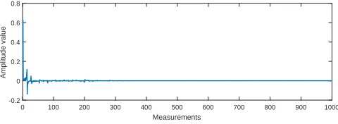
Figure 9: DCT coefficients of the second power trace inSecmatV1.
As we mentioned in Section3.3, the sparser the leakage is in one domain, the better the reconstruction performance is under the same number of observations since more key information of the leakage is compressed into these dimensions. Sparse domains are also an important topic in CS. Power traces from DPA Contest v1.1 is well sparse in DCT domain (as shown in Fig. 9). Compared with the leakage of AT89S52 micro-controller, its amplitude is smaller. The largest DCT coefficients occurs in the first dimension, and other DCT coefficients are very small.
7.2
Threshold Selection
SNR, relative error, matching degree and time consumption of OMP, CoSaMP, SP and GOMP under different sparsity are shown in Fig. 10. The SNR keeps increasing when
k < 25 then reaches about 24. It is noteworthy that SNR is relatively stable when k is from 25 to 50. CoSaMP and SP fluctuate sharply when k is greater than 50, and their performance also declines sharply. Relative error and matching degree also indicate that CoSaMP can not be able to reconstruct power traces when k >135. Since at least 3·k
atoms should be guaranteed in Λ, the time consumption of CoSaMP even drops to nearly 0 atk >100. The time consumption of SP and CoSaMP increases rapidly with sparsity, while OMP and GOMP changes little. Based on the above analysis, the k between 25 and 50 is a good choice if we want to test the percentage recovered.
We setkto 40, the relative errorαof OMP, CoSaMP and SP decreases rapidly when
0 25 50 75 100 125 150
Sparsity (k)
-10 -5 0 5 10 15 20 25 30
SNR
(a)
OMP CoSaMP
SP
GOMP
0 25 50 75 100 125 150
Sparsity (k)
0 0.5 1 1.5 2 2.5 3 3.5 4
Relative error
(b)
OMP
CoSaMP
SP
GOMP
0 25 50 75 100 125 150
Sparsity (k)
0.5 0.55 0.6 0.65 0.7 0.75 0.8 0.85 0.9 0.95 1
Matching degree
(c)
OMP CoSaMP
SP
GOMP
0 25 50 75 100 125 150
Sparsity (k)
0 1 2 3 4 5
Time (second)
(d)
OMP
CoSaMP SP
GOMP
Figure 10: SNR (a), relative error (b), matching degree (c) and time consumption (d) of OMP, CoSaMP, SP and GOMP under different sparsity.
samples leaking fromAT89S52 micro-controller, which makes the reconstruction erroreo
of power traces smaller. GOMP takes more time than other algorithms when m >300. Based on the above performance analysis,mfrom 300 to 350 is a good choice.
7.3
Performance Comparison
The second power trace is selected to perform DCT transform to compare the performance of OMP, CoSaMP, BP and GOMP, and the corresponding experimental results are shown in Fig. 12. kandmare set to 40 and 300 according to experimental results given in Section
7.2. There are more clock cycles in Fig. 7 compared with the leakage in DPA Contestv1.1 shown in Fig. 12. Due to the preprocessing of DPA Contestv1.1, its power traces are also more easy to reconstruct. The reconstructed power trace of GOMP can overlap well with the original one. Compared with the other three algorithms, the reconstruction error of GOMP is smaller and the SNR is higher (as shown in Table 3). The other 3 algorithms do not overlap well in some areas where power consumption varies distinctly. αof all 4 algorithms are larger than 0.9970. This indicates that reconstruction performance of the four algorithms is very good and meets the sampling requirements very well.
Table 3: Leakage reconstruction performance of OMP, CoSaMP, SP and GOMP on DPA Contestv1.1.
algorithms er SNR α time (second)
OMP 0.0713 22.9364 0.9988 0.010863
CoSaMP 0.0612 24.2611 0.9974 0.043958
SP 0.0692 23.2020 0.9989 0.033731
GOMP 0.0601 24.4179 0.9982 0.058839
100 200 300 400 500 600 700 800 900 1000
Number of measurements (m)
0 5 10 15 20 25 30 35 40 45 50 SNR (a) OMP CoSaMP SP GOMP
100 200 300 400 500 600 700 800 900 1000
Number of measurements (m)
0 0.1 0.2 0.3 0.4 0.5 0.6 Relative error (b) OMP CoSaMP SP GOMP
100 200 300 400 500 600 700 800 900 1000
Number of measurements (m)
0.92 0.93 0.94 0.95 0.96 0.97 0.98 0.99 1 Matching degree (c) OMP CoSaMP SP GOMP
100 200 300 400 500 600 700 800 900 1000
Number of measurements (m)
0 0.25 0.5 0.75 1 1.25 1.5 1.75 2
Time (second)
(d)
OMP CoSaMP SP GOMP
Figure 11: SNR (a), relative error (b), matching degree (c) and time consumption (d) of OMP, CoSaMP, SP and GOMP under different numbers of measurements.
0 200 400 600 800 1000
Time samples 0.005 0.01 0.015 0.02 0.025 0.03 0.035 Power consumption (a) OMP
0 200 400 600 800 1000
Time samples 0.005 0.01 0.015 0.02 0.025 0.03 0.035 Power consumption (b) CoSaMP
0 200 400 600 800 1000
Time samples 0.005 0.01 0.015 0.02 0.025 0.03 0.035 Power consumption (c) SP
0 200 400 600 800 1000
Time samples 0.005 0.01 0.015 0.02 0.025 0.03 0.035 Power consumption (d) GOMP
Figure 12: Leakage reconstruction using OMP, CoSaMP, SP and GOMP (the original power trace (blue) and reconstructed power trace (red)).
Fig. 12 are about 0.04, compared with about 0.03 of GOMP. They are all smaller than these about 0.40 in Fig. 7, since the power consumption of ASIC used in DPA Contestv1.1 is smaller than AT89S52 micro-controller. Therefore, relative error is better referential than absolute error in reconstruction performance evaluation. The relative error, SNR and matching degree in Tables2 and3 also illustrate that the reconstruction performance in Fig. 7 and Fig. 12 is similar. The power traces of DPA contestv1.1 are more compressible than these ofAT89S52 micro-controller. To achieve similar performance, we only need to collect 30% samples to reconstruct the original leakage (compared with 40% ofAT89S52
micro-controller). Moreover, the matching degree also illustrates the high performance of OMP, CoSaMP, SP and GOMP. They can quickly reconstruct the original power traces (see the time comsuption on Table 3).
0 25 50 75 100 125 150
Sparsity level(K) 0
0.1 0.2 0.3 0.4 0.5 0.6 0.7 0.8 0.9 1
Percentage recovered
(a)
OMP CoSaMP SP GOMP
0 210 230 250 270 290 310 330 350 370 390
Number of measurements(M) 0
0.1 0.2 0.3 0.4 0.5 0.6 0.7 0.8 0.9 1
Percentage recovered
(b)
OMP CoSaMP SP GOMP
Figure 13: Percentage recovered under different sparsity levels (a) and different numbers of observations (b).
In order to further compare the performance of OMP, CoSaMP, SP and GOMP, we set
k = 40,m= 300 and residual threshold to 0.04, the corresponding experimental results are shown in Fig. 13. Whenk= 40 and the step width is set to 10, it takes 5047.385466 seconds to runm from 100 to 400 (400 repetitions). Whenm= 300 and the step width is set to 5, it takes 2969.2314196 seconds to run kfrom 15 to 150 (400 repetitions). The
Pr of OMP, CoSaMP and SP is 0 whenk is from 5 to 20. k from 30 to 55 is a good
choice, which also validates our conclusion in Section7.2. Pr of GOMP increases rapidly
from 0 to 1 whenk is from 5 to 15, then drops and fluctuates. CoSaMP decreases faster than SP, and they drop to 0 atk = 100. Similar conclusion is drawn from Section 6.3. The slow performance degradation of OMP can be observed in Fig. 13, which illustrates its stability. When k = 40 and the number of observations is smaller than 200, all 4 algorithms fail to recover power traces. The absolute erroreodecreases with growth ofm.
performance of the other three algorithms improves first and then deteriorates sharply (as shown in Fig. 8 and Fig. 13). Enlarging the number of observations can improve their performance and make the locations of optimal performance move to the right. However, it is difficult to optimally balance k and m. There are currently many studies on the selection of them, such as the SWOMP shortly introduced in Section 5.2, of which k is the number of coefficients larger than half of the maximum.
8
Conclusions
The rapid increase in the bandwidth of cryptographic devices makes it difficult to sample, store and process leakages. In this paper, we introduce Compressive Sensing, a new and highly-efficient data sampling technology for side-channel leakage sampling and compare it with classical compressive sampling. Our experiments performed on power traces ob-tained from AT89S52 micro-controller and DPA contestv1.1 clearly demonstrate that CS can use a sampling rate much lower than the original one to obtain equivalent sampling performance. It projects the original power traces onto the observation space, and obtains the observation samples far below the original dimension. CS transfers a large amount of computation from sampling devices to advanced processors, so that the compute-intensive signal reconstruction can be carried out fast without distortion. In this paper, we only introduce the basic techniques of CS for leakage sampling and verify its superiority by ex-periments. There are many studies on sparse representation of signals, observation matrix design and signal reconstruction which could be applied to the leakage sampling problem. As such, we believe this work provides a new research direction in SCA which has many avenues for investigations and opportunities for further improvements.
References
[BCO04] Eric Brier, Christophe Clavier, and Francis Olivier. Correlation power analy-sis with a leakage model. InCryptographic Hardware and Embedded Systems - CHES 2004: 6th International Workshop Cambridge, MA, USA, August 11-13, 2004. Proceedings, pages 16–29, 2004.
[BD09] Thomas Blumensath and Mike E. Davies. Stagewise weak gradient pursuits.
IEEE Trans. Signal Processing, 57(11):4333–4346, 2009.
[BHvW12] Lejla Batina, Jip Hogenboom, and Jasper G. J. van Woudenberg. Getting more from PCA: first results of using principal component analysis for ex-tensive power analysis. InTopics in Cryptology - CT-RSA 2012 - The Cryp-tographers’ Track at the RSA Conference 2012, San Francisco, CA, USA, February 27 - March 2, 2012. Proceedings, pages 383–397, 2012.
[CDP15] Eleonora Cagli, Cécile Dumas, and Emmanuel Prouff. Enhancing dimension-ality reduction methods for side-channel attacks. In Smart Card Research and Advanced Applications - 14th International Conference, CARDIS 2015, Bochum, Germany, November 4-6, 2015. Revised Selected Papers, pages 15– 33, 2015.
[CDS01] Scott Shaobing Chen, David L. Donoho, and Michael A. Saunders. Atomic decomposition by basis pursuit. SIAM Review, 43(1):129–159, 2001.
[CR06] Emmanuel J. Candès and Justin K. Romberg. Quantitative robust uncer-tainty principles and optimally sparse decompositions. Foundations of Com-putational Mathematics, 6(2):227–254, 2006.
[CRT06] Emmanuel J. Candès, Justin K. Romberg, and Terence Tao. Robust uncer-tainty principles: exact signal reconstruction from highly incomplete frequen-cy information. IEEE Trans. Information Theory, 52(2):489–509, 2006.
[CT06] Emmanuel J. Candès and Terence Tao. Near-optimal signal recovery from random projections: Universal encoding strategies? IEEE Trans. Informa-tion Theory, 52(12):5406–5425, 2006.
[CW08] Emmanuel J. Candès and Michael B. Wakin. An introduction to compressive sampling. Signal Processing Magazine, IEEE, 25(2):21–30, 2008.
[DCE16] A. Adam Ding, Cong Chen, and Thomas Eisenbarth. Simpler, faster, and more robust t-test based leakage detection. In Constructive Side-Channel Analysis and Secure Design - 7th International Workshop, COSADE 2016, Graz, Austria, April 14-15, 2016, Revised Selected Papers, pages 163–183, 2016.
[DH01] David L. Donoho and Xiaoming Huo. Uncertainty principles and ideal atomic decomposition. IEEE Trans. Information Theory, 47(7):2845–2862, 2001.
[DM09] Wei Dai and Olgica Milenkovic. Subspace pursuit for compressive sensing signal reconstruction. IEEE Trans. Information Theory, 55(5):2230–2249, 2009.
[Don06] David L. Donoho. Compressed sensing. IEEE Trans. Information Theory, 52(4):1289–1306, 2006.
[dpa] Dpa contest. http://www.dpacontest.org/home/.
[DS16] François Durvaux and François-Xavier Standaert. From improved leakage de-tection to the dede-tection of points of interests in leakage traces. InAdvances in Cryptology - EUROCRYPT 2016 - 35th Annual International Conference on the Theory and Applications of Cryptographic Techniques, Vienna, Austria, May 8-12, 2016, Proceedings, Part I, pages 240–262, 2016.
[DTDS12] David L. Donoho, Yaakov Tsaig, Iddo Drori, and Jean-Luc Starck. Sparse solution of underdetermined systems of linear equations by stagewise orthog-onal matching pursuit. IEEE Trans. Information Theory, 58(2):1094–1121, 2012.
[GHT05] Catherine H. Gebotys, Simon Ho, and C. C. Tiu. EM analysis of rijndael and ECC on a wireless java-based PDA. In Cryptographic Hardware and Embedded Systems - CHES 2005, 7th International Workshop, Edinburgh, UK, August 29 - September 1, 2005, Proceedings, pages 250–264, 2005.
[GN03] Rémi Gribonval and Morten Nielsen. Sparse representations in unions of bases. IEEE Trans. Information Theory, 49(12):3320–3325, 2003.
[GSTV06] Anna C. Gilbert, Martin J. Strauss, Joel A. Tropp, and Roman Vershynin. Algorithmic linear dimension reduction in the l_1 norm for sparse vectors.
[HTWM10] Zachary T. Harmany, Daniel Thompson, Rebecca Willett, and Roummel F. Marcia. Gradient projection for linearly constrained convex optimization in sparse signal recovery. In Proceedings of the International Conference on Image Processing, ICIP 2010, September 26-29, Hong Kong, China, pages 3361–3364, 2010.
[Kas91] B Kashin. The widths of certain finite dimensional sets and classes of smooth functions, izvestia 41 (1977), 334–351. MR0481792 (58: 1891), 1891.
[KJJ99] Paul C. Kocher, Joshua Jaffe, and Benjamin Jun. Differential power anal-ysis. In Advances in Cryptology - CRYPTO ’99, 19th Annual International Cryptology Conference, Santa Barbara, California, USA, August 15-19, 1999, Proceedings, pages 388–397, 1999.
[LD06] Chinh La and Minh N. Do. Tree-based orthogonal matching pursuit algorithm for signal reconstruction. InProceedings of the International Conference on Image Processing, ICIP 2006, October 8-11, Atlanta, Georgia, USA, pages 1277–1280, 2006.
[Mal09] Arian Maleki. Coherence analysis of iterative thresholding algorithms.CoRR, abs/0904.1193, 2009.
[MOP07] Stefan Mangard, Elisabeth Oswald, and Thomas Popp. Power analysis at-tacks - revealing the secrets of smart cards. Springer, 2007.
[MRSS18] Amir Moradi, Bastian Richter, Tobias Schneider, and François-Xavier Stan-daert. Leakage detection with the x2-test. IACR Trans. Cryptogr. Hardw. Embed. Syst., 2018(1):209–237, 2018.
[MZ93] Stéphane Mallat and Zhifeng Zhang. Matching pursuits with time-frequency dictionaries. IEEE Trans. Signal Processing, 41(12):3397–3415, 1993.
[NT10] Deanna Needell and Joel A. Tropp. Cosamp: iterative signal recovery from incomplete and inaccurate samples. Commun. ACM, 53(12):93–100, 2010.
[NV09] Deanna Needell and Roman Vershynin. Uniform uncertainty principle and signal recovery via regularized orthogonal matching pursuit. Foundations of Computational Mathematics, 9(3):317–334, 2009.
[NV10] Deanna Needell and Roman Vershynin. Signal recovery from incomplete and inaccurate measurements via regularized orthogonal matching pursuit.J. Sel. Topics Signal Processing, 4(2):310–316, 2010.
[OSW+17] Changhai Ou, Degang Sun, Zhu Wang, Xinping Zhou, and Wei Cheng.
Man-ifold learning towards masking implementations: A first study. IACR Cryp-tology ePrint Archive, 2017:1112, 2017.
[PM00] Erwan Le Pennec and Stéphane Mallat. Image compression with geometrical wavelets. InProceedings of the 2000 International Conference on Image Pro-cessing, ICIP 2000, Vancouver, BC, Canada, September 10-13, 2000, pages 661–664, 2000.
[SA08] François-Xavier Standaert and Cédric Archambeau. Using subspace-based template attacks to compare and combine power and electromagnetic infor-mation leakages. InCryptographic Hardware and Embedded Systems - CHES 2008, 10th International Workshop, Washington, D.C., USA, August 10-13, 2008. Proceedings, pages 411–425, 2008.
[SM15] Sujit Kumar Sahoo and Anamitra Makur. Signal recovery from random mea-surements via extended orthogonal matching pursuit. IEEE Trans. Signal Processing, 63(10):2572–2581, 2015.
[SMY09] François-Xavier Standaert, Tal Malkin, and Moti Yung. A unified framework for the analysis of side-channel key recovery attacks. InAdvances in Cryp-tology - EUROCRYPT 2009, 28th Annual International Conference on the Theory and Applications of Cryptographic Techniques, Cologne, Germany, April 26-30, 2009. Proceedings, pages 443–461, 2009.
[SNG+10] Youssef Souissi, Maxime Nassar, Sylvain Guilley, Jean-Luc Danger, and
Flo-rent Flament. First principal components analysis: A new side channel dis-tinguisher. InInformation Security and Cryptology - ICISC 2010 - 13th In-ternational Conference, Seoul, Korea, December 1-3, 2010, Revised Selected Papers, pages 407–419, 2010.
[SYZ08] Florian M. Sebert, Leslie Ying, and Yi Ming Zou. Toeplitz block matrices in compressed sensing. CoRR, abs/0803.0755, 2008.
[TG07] Joel A. Tropp and Anna C. Gilbert. Signal recovery from random measure-ments via orthogonal matching pursuit. IEEE Trans. Information Theory, 53(12):4655–4666, 2007.
[Tro04] Joel A. Tropp. Greed is good: algorithmic results for sparse approximation.
IEEE Trans. Information Theory, 50(10):2231–2242, 2004.