Implementation of Efficient Adaptive filter Algorithms for WSN Applications

Implementation of Efficient Adaptive filter

Algorithms for WSN Applications

Dumpa. Prasad1, S.D.Dixit2

Research Scholar, Dept of ECE, University of Allahabad, UP, India1

Professor, Dept of ECE, University of Allahabad, UP, India2

ABSTRACT: In wireless sensor networks (WSN), the nodes are low powered gadgets and therefore designing a low

power WSN is particularly primary for getting longer lifetime. Wireless Sensor Networks are more and more being employed for monitoring and sensing in severe environments similar to factories and offshore platforms. The aim of this paper is to be study, analyse and evaluate on 3 distinctive forms of adaptive filtering approaches comparable to Least mean square (LMS), Recursive Least square (RLS) and fast transversal recursive least-squares (FT-RLS) algorithms. This algorithm is designed to provide similar performance to the standard RLS algorithm at the same time decreasing the computation order. This is finished with the assistance of a combination of 4 transversal filters used in unity. Finite precision results are additionally briefly stated. Simulations are carried out with each algorithm to compare both the computational burden as well as the efficiency of each scheme for adaptive noise cancellation. Simulations exhibit that FT-RLS presentscomparableperformance with respect to the conventional RLS furthermore to an enormous reduction in computation time for better order filters. Implementation elements of those algorithms, their computational complexity and mean square error (MSE) are examined. These algorithms use small input and output delay. Here, the adaptive behaviour of the algorithms is analyzed. Lately, adaptive filtering algorithms have aagreeabletrade-off between the complexity and the convergence speed.

KEYWORDS: Adaptive Filters, LMS, RLS, FT-RLS, least-squares, wireless sensor networks

I. INTRODUCTION

Wireless sensor networks (WSNs) are a class of distributed computing and communication systems that are an integral part of the physical space they inhabit [1]. This type of network is characterized by nodes with a low profile, having limited computational power and sparse energy resources, which have the ability to collaborate with each other, and to sense, reason, and react to the world that surrounds them. Recent advances in this field have enabled the development of wireless sensor networks, the functionality of which rely on the collaborative effort of a large number of tiny, lowcost, low-power, multi-functional sensor nodes that are able to communicate un-tethered over short distances [2,3]. More- over, engineering or predetermining the positions of the nodes is not necessary. This allows random deployment in hostile environments or disaster-relief operations, a unique feature that accounts for rendering these network types an integral part of modern life. Smart environments represent the next evolutionary development step in the automation of building, utility, industrial, home, shipboard, and transportation systems [4]. This bridge to the physical world has enabled a growing bouquet of added-value services, ranging from health to military and security, such as target tracking, environmental control, habitat monitoring, source detection and localization, vehicular and traffic monitoring, health monitoring, building and industrial monitoring, etc. [5,]. On the other hand, wireless sensor networks display certain undesirable or hard-to-deal-with features. These include power limitations, frequently changed topology, broadcast communication, susceptibility to failure, and low memory, while their architecture calls for protocols and algorithms with self-organizing capabilities [2].

Fig 1: Hierarchy of Adaptive Filters

Adaptive techniques use algorithms, which enable the adaptive filter to adjust its parameters to produce an output that matches the output of an unknown system. This algorithm employs an individual convergence factor that is updated for each adaptive filter coefficient at each iteration.

II. FAMILIES OF LMS AND RLS

A. LEAST MEAN SQUARE (LMS) ALGORITHM

The Least Mean Square (LMS) algorithm, introduced by Widrow and Hoff in 1960, is a linear adaptive filtering algorithm, which uses a gradient-based method of steepest decent. The LMS algorithm uses the estimates of the gradient vector from the available data and incorporates an iterative procedure that makes successive corrections to the weight vector in the direction of the negative of the gradient vector which eventually leads to the minimum mean square error.

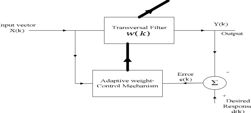
The LMS algorithm consists of two basic processes. These are filtering process and adaptive process. A filtering process involves computing the output of a linear filter in response to an input signal and generating an estimation error by comparing this output with a desired response. An adaptive process involves the automatic adjustment of the parameters of the filter in accordance with the estimation error. The combination of these two processes working together constitutes a feedback loop.

) (k w

The LMS algorithm is the simplest and is the most universally applicable adaptive algorithm to be used. This algorithm uses a special estimate of the gradient that is valid for the adaptive linear combiner. This algorithm is important because of its simplicity and ease of computation. It does not require explicit measurement of correlation functions, nor does it

involve matrix inversion. Accuracy is limited by statistical sample size, since the weight values found are based on real-time measurements of input signals.

Algorithm Summary:

The LMS algorithm [1] for a pth order algorithm can be summarized as Parameters: P = filter order

µ = step size

Initialization: ĥ (0) = 0

Computation: For n = 0, 1, 2...

X(n) = [x(n), x(n - 1), …, x(n – p + 1)]T e(n) = d(n) – ĥH(n) X(n)

ĥ (n+1) = ĥ(n) + µ e*(n) X(n)

B. THE RECURSIVE LEAST SQUARES (RLS) ALGORITHM

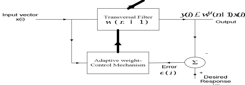
The RLS algorithm as a natural extension of the method of least squares to develop and design of adaptive transversal filters such that, given the least squares estimate of the tap-weight vector of the filter at iteration n1. Therefore, we may compute the updated estimate of the vector at iteration

n

An important feature of this algorithm is that its rate of convergence is typically an order of magnitude faster than that of the simple LMS algorithm. However, this improvement of performance is achieved at the expense of an increase in computational complexity of the RLS algorithm.

) 1 (n  w ) ( ) 1 ( )

(i w n xi

y  H 

) (i e

Fig 3: Block diagram representation of the RLS algorithm

Algorithm Summary:

Initialize the algorithm by setting

 

0



0



w

 

I

P

0





_





0

For each instant time, n = 1, 2, 3,…, compute

 

n



P



n



1

  

x

n



 

 

   

n

n

x

n

n

k











 

n

w



n



k

   

n

e

n

w







 

1

 

n



P



n



1





k

   

n

x

n

P



n



1



P





C. TRANSFORM DOMAIN ADAPTIVE FITTERS( DCT-LMS, DFT –LMS AND INCREMENTAL-LMS)

The convergence rate of LMS (Least mean square) type filter is dependent on the Autocorrelation matrix of the input data and on the eigen value spread of the covariance matrix of the regressor data [9]. The mean square error (MSE) of an adaptive filter using LMS algorithm decreases with time as sum of the exponentials, whose time constants are inversely proportional to the eigen value of the auto correlation matrix of input data [10]. The smaller eigen value of autocorrelation matrix of the input results slower convergence mode and larger eigen values limit on the maximum learning rate that can be chosen without encountering stability problem. Best convergence and learning rate results when all the eigen values of the input autocorrelation matrix are equal i.e. Autocorrelation matrix should be in the form of a constant multiplication with the identity matrix [9]. Practically the input data’s are colored and the Eigen values of autocorrelation matrix vary from smallest to the largest. The filter response can be improved by prewhitening the data, but for this the autocorrelation of the input data should be known. It is difficult to know the autocorrelation of the input data. It can be achievable by using unitary transformation, such as discrete cosine transform (DCT), discrete Fourier transform (DFT) etc. These transformation have de-correlation properties that improves the convergence performance of LMS for correlated input data [9].

Transform domain (which is also called frequency domain) can be applied in two ways one is block wise frequency domain algorithm other is non-block wise frequency domain algorithm [11]. In block wise frequency domain algorithm a block of input data is first transformed then input to the incremental LMS algorithm and in non-block or real time algorithm the data are continuously transformed by a fixed data-independent transform to de-correlate the input data [10]. DFT-LMS algorithm was first introduced by Narayan belongs to a simplest algorithm family because of the exponential nature [12]. But in many practical situation it was found that DCT-LMS performs better than that of DFT-LMS and other transform domain [10].In this paper we interpret the incremental DFT-LMS using DCT/DFT algorithm and found that it produce better convergence and performance than previous.

III.PROPOSEDAPPROACHES

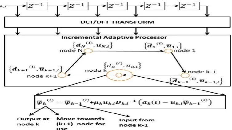
In this paper initially we apply DCT-LMS and DFT-LMS algorithm in incremental method, then we found that the DCT-LMS not only gives better convergence but also gives better performance than that of rest. In in frequency domain incremental, the process is same as the incremental method, only the difference is instead taking the entire parameter time domain here we will take in frequency domain and introduce a term D in the weight updation equation. That is here first the data transform to frequency domain then apply to incremental strategies using the respective algorithm. The block diagram of frequency domain incremental strategy shown in Fig.4.

A. FAST-TRANSVERSAL RECURSIVE LEAST-SQUARES

The Fast Transversal RLS (FT-RLS) filter is designed toprovide the solution to the filtering problem with performance equal to the standard recursive least-squares (RLS) algorithm.In addition, the FT-RLS filter provides this solution with reduced computational burden which scales linearly with thefilter order. This makes it a very attractive solution in real-time noise cancellation applications. The FT-RLS developmentis based on the derivation of lattice-based least-squares filters but has the structure of four transversal filters working togetherto compute update quantities reducing the computational complexity [6]. The full derivation of the FT-RLS algorithm canbe found in [7]. The four transversal filters used for forming the update equations are:

1) Forward Prediction: The forward prediction transversalfilter computes the forward filter weights in such amanner that minimizes the prediction error (in the leastsquares sense) of the next input sample based on theprevious input samples. This filter also computes theprediction error of estimation using both a priori anda posterior filter weights, in addition to the minimumweighted least squares error for this forward prediction.

2) Backward Prediction: The backward prediction transversal filter computes backward filter weights in such a manner that minimizes the prediction error (in the leastsquares sense) of the u(n¡M) sample using the vector input ub(n) = [u(n)u(n ¡ 1) ………… u(n ¡ M + 1)]T . This filter will also compute the respective prediction error of estimation using both a priori and a posterior filter weights, in addition to the minimum weighted leastsquares error for this backward prediction.

3) Conversion Factor: The gain computation transversal filter is used to recursively compute a gain vector which is used to updating the forward, backward and joint process estimation filter weights. As such this filter also provides recursive computation of the factors relating a priori and a posteriori error quantities.

4) 4) Joint-Process Estimation: The joint-process estimation transversal filter computes filter weights in such a manner that the error between the estimated signal and the desired input signal (d(n)) is minimized. It is the joint process estimation weights that are equivalent to filter weights in other adaptive filtering algorithms.

The FT-RLS algorithm unfortunately leads to numerical instability in a finite precision environment. The details of this instability are studied in detail in [8]. There have been several methods proposed to create a stabilized version of FT-RLS. In general, these methods involve expressing certain update equations in different forms. With high precision these quantities are identical, however become unequal in finite precision. The difference between the values is often used as a measure of the numerical sensitivity. One solution is to utilize a weighted average of the update equations. This is the solution proposed in [8]. Using calculation redundancy in several of these quantities provides numerical stability in the presence of finite precision. The result of this gives rise to the proposed stabilized FT-RLS [4], which requires more calculations per iteration to operate, however is more numerical robust compared to FT-RLS and maintains scaling of O(M).

B. STABILIZED FAST TRANSVERSAL RLS ALGORITHM

Although the fast transversal algorithms proposed in the literature provide a nice solution to the computational complexity burden inherent to the conventional RLS algorithm, these algorithms are unstable when implemented with finite-precision arithmetic. Increasing the word length does not solve the instability problem. The only effect of employing a longer word length is that the algorithm will take longer to diverge. Earlier solutions to this problem consisted of restarting the algorithm when the accumulated errors in chosen variables reached prescribed thresholds [14]. Although the restart procedure would use past information, the resulting performance is suboptimal due to the discontinuity of information in the corresponding deterministic correlation matrix.

solutions [15]-[16], only a single quantity was chosen to introduce the redundancy. Later, it was shown that at least two quantities are required in order to guarantee the stability of the FTRLS algorithm [13]. Another relevant question is where the error should be fed back inside the algorithm. Note that any point could be chosen without affecting the behaviour of the algorithm when implemented with infinite precision, since the feedback error is zero in this case. A natural choice is to feed the error back into the expressions of the quantities that are related to it. That means for each quantity in which redundancy is introduced, its final value is a combination of the two forms of computing it. The FTRLS algorithm can be seen as a discrete-time nonlinear dynamic system [13]: when finite precision is used in the implementation, quantization errors will rise. In this case, the internal quantities will be perturbed when compared with the infinite-precision quantities. When modeling the error propagation, a nonlinear system can be described that, if properly linearized, allows the study of the error propagation mechanism. Using an averaging analysis, which is meaningful for stationary input signals, it is possible to obtain a system characterized by its set of eigenvalues whose dynamic behaviour is similar to that of the error propagation behaviour when k →∞ and (1−λ) → 0.Through these eigenvalues, it is possible to determine the feedback parameters as well as the quantities to choose for the introduction of redundancy. The objective here is to modify the unstable modes through the error feedback in order to make them stable [13]. Fortunately, it was found in [13] that the unstable modes can be modified and stabilized by the introduced

error feedback. The unstable modes can be modified by introducing redundancy in γ(k, N) and eb(k, N).

From the Table I show that, the performance of FT- RLS adaptive algorithm is high as compared to other algorithm due to the less mean-square error (MSE).

Table I Performance Comparison of Adaptive Algorithms

S.No. Algorithms MSE Complexity Stability

1. LMS 1.5*10-2 _{2N+1 LessStable}

2. NLMS 9.0*10-3 _{3N+1 Stable}

3. RLS 6.2*10-3 _4N2 _HighStable

4 FT-RSL 4.2*10-3 _2N2 Very High

Stable

IV. SIMULATION RESULTS

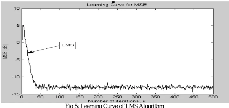
In order to compare the performance of FT-RLS versus the standard RLS and LMS, both algorithms were implemented in MATLAB in an adaptive noise cancellation and WSN application.Simulation results are presented for the case of MSE versus number of iterations. The number of algorithm iterations is set of 500.

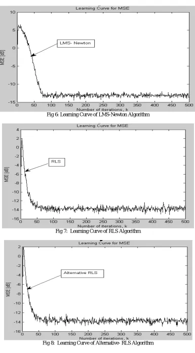
This simulation studies the use of the LMS algorithm for adaptive equalization of a linear dispersive channel that produces distortion. Here we review and compare all the techniques that were studied in this chapter. The LMS, RLS and Allternate RLS techniques developed are compared with each other . The MSE is taken as the performance metric which gives the convergence rate. It is obvious that percentage of saving the computations degrades the performance. All the techniques mentioned here are compared for 70%, 50%, and 30% coefficient update. The following results give the clear analysis over each technique.

Fig 6: Learning Curve of LMS-Newton Algorithm

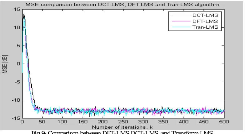
By performing a simulation to compare with the convergence and performance of transform-LMS, DCTLMS, DFT-LMS, it is found that the prewhitening filter gives better result than that of rest as shown in Fig.9.

Fig 9: Comparison between DFT-LMS DCT-LMS, and Transform LMS

For comparisonpurpose simulation is performed to compare the convergence rate and performance of all the algorithm i.e. adaptive incremental method, incremental steepest descent solution, and DCT-LMS and DFT-LMS algorithm using incremental method. It is found that the convergence rate and performance of DCT-LMS algorithm using incremental method gives better result than that of rest algorithm. The MSE (mean square error), comparison of the entire algorithm as shown in Fig.10.

Fig 10: Transient MSE performance at node 1 for incremental adaptive solution

Fig 11: MSE comparison between Fast-RLS, Stable-RLS, RLS and LMS algorithm

V. CONCLUSION

In this paper, an overview of the RLS algorithm was provided. After thorough simulations, it is clear that the FT-RLS algorithm is a highly suitable solution for adaptive filtering applications where a large filter order is required without sacrificing the performance offered by the standard RLS algorithm in the presence of noise. It concludes that the best adaptive algorithm is FT-Recursive Least Square according to the Performance Comparison of Adaptive Algorithms Table.1 and graphs of MSE.Here we can say that in the comparison of the LMS, RLS, DCT-LMS, INCREMENTAL-LMS and FT-RSL algorithm, the FT-RLS approach offers faster convergence and smaller error with respect to the unknown system.

REFERENCES

[1] C. N. Raghavendra, K. M. Sivalingham, and T. Znati, Wireless Sensor Networks, New York, Springer Science and Business Media Inc., 2004. [2] I. F. Akyildiz, W. Su, Y. Sankarasubramaniam, and E.Cayirci,“Wireless Sensor Networks: A Survey,” Computer Networks Journal, 18, 2, 2002, pp. 393-422.

[3] S. Misra, S. C. Misra, and I. Wounqanq, Guide to Wireless Mesh Networks, Berlin, Springer, December 2010.

[4] F. L. Lewis, “Wireless Sensor Networks,” in Diane Cook and Sajal Das (eds.), Smart Environments: Technologies, Protocols and Applications, New York, John Wiley and Sons, 2004.

[5] E. H. Callaway, Wireless Sensor Networks: Architectures and Protocols, Boca Raton, FL, CRC Press, 2004. [6] P. S. R. Diniz, Adaptive Filtering: Algorithms and Practical Implementation. Kluwer Academic Publishers, 1997.

[7] J. Cioffi and T. Kailath, “Fast Recursive-Least-Squares, Transversal Filters for Adaptive Filtering,” IEEE Trans. Acoust., Speech, Signal Processing, vol. 32, pp. 304–337, 1984.

[8] D. T. M. Slock and T. Kailath, “Numerically Stable Fast Transversal Filters for Recursive Least Squares Adaptive Filtering,” IEEE Trans. on Signal Processing, vol. 39, pp. 92–113, Jan 1991.

[9] A. H. Sayed, Fundamentals of adaptive filtering, John Wiley \& Sons, 2003.

[10] F. Beaufays, "Transform-domain adaptive filters: an analytical approach," Signal Processing, IEEE Transactions on, vol. 43, no. 2, pp. 422-431, 1995.

[11] J. J. Shynk and others, "Frequency-domain and multirate adaptive filtering," IEEE Signal Processing Magazine, vol. 9, no. 1, pp. 14-37, 1992. [12] S. Narayan, A. M. Peterson and M. J. Narasimha, "Transform domain LMS algorithm," Acoustics, Speech and Signal Processing, IEEE

Transactions on, vol. 31, no. 3, pp. 609-615, 1983.

[13]. D. T. M. Slock and T. Kailath, “Numerically stable fast transversal filters for recursive least squares adaptive filtering,” IEEE Trans. on Signal Processing, vol. 39, pp. 92-113, Jan. 1991.

[14]. J. M. Cioffi and T. Kailath, “Fast, recursive-least-squares transversal filters for adaptive filters,” IEEE Trans. on Acoust., Speech, and Signal Processing, vol. ASSP-32, pp. 304-337, April 1984.

[15]. J.-L. Botto and G. V. Moustakides, “Stabilizing the fast Kalman algorithms,” IEEE Trans. on Acoust., Speech, and Signal Processing, vol. 37, pp. 1342-1348, Sept. 1989.