Article
1
Elucidating Cellular Population Dynamics by
2
Molecular Density Function Perturbations
3
Thanneer Malai Perumal 1 and Rudiyanto Gunawan 2,3,*
4
1 Sage Bionetworks, Seattle, Washington, USA; [email protected]
5
2 Institute for Chemical and Bioengineering, ETH Zurich, Zurich, Switzerland; [email protected]
6
3 Swiss Institute of Bioinformatics, Lausanne, Switzerland
7
* Correspondence: [email protected]; Tel.: +41-44-633-2134
8
Abstract: Studies performed at single-cell resolution have demonstrated the physiological
9
significance of cell-to-cell variability. Various types of mathematical models and systems analyses
10
of biological networks have further been used to gain a better understanding of the sources and
11
regulatory mechanisms of such variability. In this work, we present a novel sensitivity analysis
12
method, called molecular density function perturbation (MDFP), for the dynamical analysis of
13
cellular heterogeneity. The proposed analysis is based on introducing perturbations to the density
14
or distribution function of the cellular state variables at specific time points, and quantifying how
15
such perturbations affect the state distribution at later time points. We applied the MDFP analysis
16
to a model of signal transduction pathway involved in TRAIL (tumor necrosis factor-related
17
apoptosis-inducing ligand)-induced apoptosis in HeLa cells. The MDFP analysis showed that
18
caspase-8 activation regulates the timing of the switch-like increase of cPARP (cleaved
19
poly(ADP-ribose) polymerase), an indicator of apoptosis. Meanwhile, the cell-to-cell variability in
20
the commitment to apoptosis depended on mitochondrial outer membrane permeabilization
21
(MOMP) and events following MOMP, including the release of Smac (second
22
mitochondria-derived activator of caspases) and cytochrome-C from mitochondria, the inhibition
23
of XIAP (X-linked inhibitor of apoptosis) by Smac and the formation of apoptosome.
24
Keywords: mathematical modeling; biological networks; sensitivity analysis; programmed cell
25
death; single cell dynamics; cell population
26
27
1. Introduction
28
Advances in single-cell profiling technology and the application of this technology to study
29
biology at single-cell resolution have demonstrated the ubiquity and functional role of cell-to-cell
30
variability in physiological processes, such as programmed cell death (apoptosis) and stem cell
31
differentiation [1–3]. Besides genetic, epigenetic and environmental factors, the cellular
32
heterogeneity observed in a given cell population has also been attributed to the inherent stochastic
33
dynamics of cellular processes. For example, gene transcriptional processes have been shown to
34
occur in stochastic (random) bursts [4–6]. Many modeling frameworks have been used to capture
35
cellular heterogeneity, for example by using ensemble models (EM) of ordinary differential
36
equations (ODEs) [7,8], population balance models (PBMs) [9], stochastic ordinary differential
37
equations (SDEs) [10,11], and chemical master equations (CMEs) [12–14]. In these models, the
38
cell-to-cell variability is described by a probability density or distribution function of cell state
39
variables. Systems analyses have also been developed and applied to gain insights into the dynamics
40
of cell state distribution. For example, several types of parameter sensitivity analysis, including
41
SOBOL sensitivity [15], DGSM [16], Glocal analysis [17], extended Fourier Amplitude Sensitivity
42
Test (eFAST) [18], and stochastic sensitivity analysis [19–25], have been used to identify the
43
rate-controlling or bottlenecking processes based on dynamic models of cell distribution.
44
Parameter sensitivity analysis (PSA) is a common systems analysis that is used to elucidate the
45
dependence of systems behavior on system parameters [26,27]. In the PSA, we compute sensitivity
46
coefficients whose magnitude describes how much system states vary with changes in one or a
47
combination of system parameters. A large sensitivity magnitude means that the system behavior
48
strongly depends on changes in the corresponding parameter(s), an indication of a rate-limiting
49
process. In several publications [28–30], we have shown that the traditional PSA, derived using static
50
perturbations to system parameters, may lead to incorrect conclusions when the rate-limiting
51
process changes with time. For this reason, we have created a new class of sensitivity analysis based
52
on impulse perturbations on parameters and states, called impulse parameter sensitivity analysis
53
(iPSA) and Green’s function matrix (GFM) analysis, respectively [28–30]. By introducing impulse
54
perturbations at different times, the new sensitivity analyses are able to reveal not only which
55
processes are rate-limiting, but also when they become rate-limiting.
56
In this work, we adapted the concept of impulse perturbation based PSA for the dynamical
57
analysis of cell-to-cell variability. The new sensitivity analysis, called molecular density function
58
perturbation (MDFP), is based on time-varying perturbations to the probability density or
59
distribution function of the cell state variables. The MDFP sensitivity coefficients are defined using
60
distribution distances in order to account for changes in the cell state distribution beyond the
61
first-order moment (i.e., population mean). We applied the MDFP analysis to a model of
62
programmed cell death in HeLa cell population [31] and identified key regulators of apoptotic
63
decision making.
64
2. Material and Methods
65
Sensitivity analysis of dynamic models of cell distribution has received much interest in recent
66
times along with the rise of systems biology and the increasing attention to single-cell analysis.
67
Novel PSA methods have been developed for the CME models of biological networks [19–25]. Here,
68
the sensitivity coefficients describe changes in the mean of cell state distribution caused by
69
infinitesimal (local) perturbations to the parameter values. Methods for global sensitivity analysis
70
have also been adapted for analyzing cell distribution sensitivities, such as sampling-based Partial
71
Rank Correlation Coefficient (PRCC) and variance-based eFAST [18]. Despite their differences, the
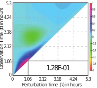
72
aforementioned sensitivity analyses and the corresponding sensitivity coefficients are based on
73
static or persistent parameter perturbations. As we have demonstrated previously, such analysis is
74
incapable of elucidating any dynamic transitions of the bottlenecking process [28–30].
75
3.1. Molecular Density Function Perturbation (MDFP) analysis
76
In the following, we formulate the molecular density function perturbation (MDFP) analysis. In
77
MDFP, we describe the cell distribution using a probability density function (PDF), denoted by
78
( , ), where ∈ ℝ denotes the cell state vector and t denotes the time variable. This description
79
of cell distribution is flexible enough to accommodate mathematical modelling frameworks that are
80
commonly used to simulate cell-to-cell variability, including EMs, PBMs, SDEs and CMEs. In
81
biological network models, the cell state is typically defined by the concentrations of biomolecules.
82
By definition, the (n-tuple) integral of the PDF ( , ) gives the fraction of cell population at
83
time t whose states (concentrations) satisfy ≤ ≤ . The basic premise of the MDFP analysis is the
84
same as that of impulse perturbation based sensitivity analysis, specifically the GFM analysis [28],
85
which is to introduce a perturbation to the cell state at time and quantify the effect of this
86
perturbation at a later time t ( ≥ ). But, the MDFP analysis uses perturbations to the PDF of the cell
87
state.
88
In deriving the MDP sensitivity coefficients, we start with following relationship:
89
( , )= | ( , | , ) ( , ). (1)
The PDF | ( , | , ), also known as the transitional probability or the propensity function, gives
90
the conditional PDF of x at time t given that the cell state is at time ( ≥ ). In the following, we
91
consider introducing a mean-shift perturbation to the PDF at time to give:
( , )= − , , (2)
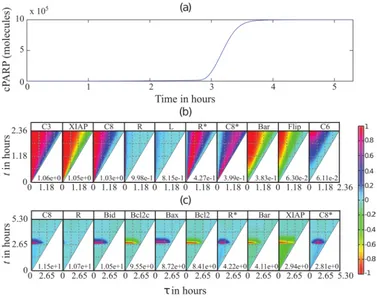
where denotes the perturbed state variables and denote the j-th column of the identity matrix.
93
Note that the PDF ( , ) corresponds to the PDF ( , ) with a positive mean-shift of , i.e.
94
= + . Given the perturbed PDF ( , ) at time and the propensity function
95
| ( , | , ), we can define the perturbed PDF of the cell state at time t, denoted by , ( , ), as
96
follows:
97
, ( , )=
| ( , | , ) ( , ). (3)
Note that the following equality applies
98
, ( , )= ( , )
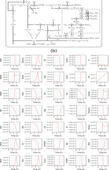
. (4)
In the MDFP analysis, we employ a distribution distance metric to quantify the magnitude of
99
PDF changes caused by the perturbations. Several metrics of distribution distance are available, such
100
as the Kullback-Leibler distance (Δ ), Jeffrey distance (Δ ), Jennson-Shanon divergence (Δ ),
101
engineering metric (Δ ), Kolmogorov-Smirnov distance (Δ ) and Cramer-von Mise distance (Δ ).
102
The first four of the aforementioned distribution distances are based on the difference between two
103
PDFs, while the remaining two are based on the difference between the cumulative density
104
functions (CDFs). For the analysis of programmed cell death model below, we used the Cramer von
105
Mise distance: (see Supplementary Material S1 for the mathematical definitions of the other
106
distribution distances)
107
Δ ( )|| ( ) = ( )− ( ) , (5)
which in our experience, gives more reliable sensitivity coefficient calculations. The variable ( )
108
denotes the CDF of the PDF ( ), i.e. ( )= ( ) .
109
Following the common definition of sensitivity coefficients [32], we computed the MDFP
110
sensitivity coefficients as the ratio of the changes in the PDF of the cell state at time t and the
111
perturbation introduced at time . The sensitivity coefficients are evaluated for a particular cell state
112
variable of interest (the i-th element of x) with respect to a perturbation to on the state
113
variable , as follows:
114
, ( , )=
( ) ( )
, ( ,)|| ,( ,)
, || ,
, (6)
where (∙) gives the sign of the argument variable and Δ ( ) denotes the change in the mean
115
of the state variable at time t. The function ,( , ) denotes the marginal PDF of , ( , )
116
with the following definition:
117
, ( , )= , ( , )
~. (7)
The integration in Eq. (7) is performed over all state variable ’s except for . Note that the
118
sensitivity coefficient in Eq. (6) above is motivated by the centered difference approximation [32],
119
where the sensitivity coefficients are computed using positive and negative perturbations to the
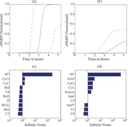
120
system.
121
The definition of the MDFP sensitivity coefficients is analogous to the Green’s function matrix
122
(GFM) sensitivity [28,32]. We can visualize , ( , ) using a heatmap as shown in Figure 1. The
123
magnitudes of the sensitivities represent the degree of importance, while the signs of the sensitivity
124
coefficients reflect the direction of the mean change. A positive sensitivity coefficient indicates that
125
the mean change of at time t is in the same direction as the mean-shift perturbation to at time
126
. One can further use the magnitudes of the sensitivity coefficients to rank state variables (at time )
according to the degree of influence on a particular state variable (at time t), where larger sensitivity
128
magnitudes indicate a higher importance.
129
In the case study, we considered an ensemble of ODE models, where each model represents one
130
cell in a cell population. The models in the ensemble share the same ODEs and parameters, but have
131
different initial states. The ODE model follows the general formula:
132
( , )
= ( , ), (8)
where denotes the vector of model parameters and ( , ) is a vector-valued nonlinear function.
133
The distribution of the initial conditions is given by the PDF , . The sensitivity coefficients
134
were computed using a Monte Carlo approach, where we simulated an ensemble of ODE models
135
with a random sample generated from , as initial conditions. The model simulation of each
136
randomly sampled initial condition represented the state trajectory of one cell in the cell population.
137
For the computation of , ( , ), we introduced a perturbation to the state variable for each
138
of the cells in the ensemble at selected time points , and simulated the perturbed state trajectory of
139
until the desired time ( ≥ ). We constructed the marginal PDFs or CDFs of the state variables
140
using a kernel density estimator with leave-one-out cross validation [33].
141
142
Figure 1. A heatmap of MDFP sensitivity coefficient. The x-axis represents the time at which
143
perturbation is introduced, while the y-axis represents the observation time t. The MDFP coefficient
144
in the heatmap is scaled such that the magnitude falls within ±1, and the scaling factor is reported in
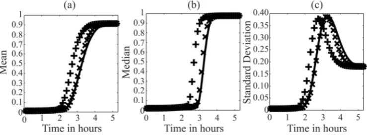
145
the lower right corner of the plot. The sensitivity values for are set to zero for causal systems.
146
3.2. Green Function Matrix analysis
147
We compared the MDFP analysis to a related sensitivity analysis based on the GFM. Like the
148
MDFP analysis, the GFM analysis introduces time-dependent perturbations to the state variables.
149
The GFM sensitivity coefficients are calculated by directly differentiating the ODE model in Eq. (8)
150
as follows: [28]
151
( )
( ) = ( , )=
( , )
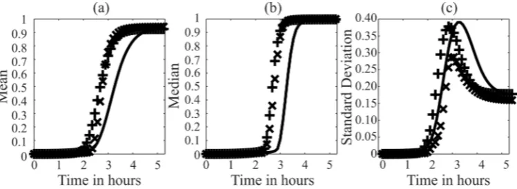
; ( , )= (10)
where ( , ) is the sensitivity matrix and is the identity matrix. The ( , )-th
152
element of ( , ), i.e. , ( , )= ( )⁄ ( ), gives the sensitivity of the state ( ) with
153
respect to perturbations to the state ( ) ( ≥ ). In the case study below, we normalized the
154
sensitivity coefficients as follows:
155
, ( , )= , ( , )
( )
( ) (11)
We computed the GFM sensitivity coefficients following the procedure described in the original
156
publication [28].
3. Results
159
3.1. TRAIL-induced cell death model of HeLa cells
160
Figure 2 depicts the signaling network associated with extrinsically-induced apoptosis by
161
tumor necrosis factor related apoptosis-inducing ligand (TRAIL). The ODE model comprises 58
162
species, 28 reactions and 70 kinetic parameters [34] (see Supplementary Material S2 for details on the
163
initial conditions, parameter values and rate equations). The model parameters and initial conditions
164
were determined by parameter fitting to experimental data of single-cells and cell populations from
165
cell imaging, flow cytometry, and immunoblotting experiments [31,35,36]. The model describes the
166
key mechanisms for the activation of endogenous executioner caspase-3 (C3*) and the subsequent
167
cleavage of poly(ADP-ribose) polymerase (PARP) [35]. Specifically the model includes four major
168
pathways: (i) the upstream pathway, representing TRAIL-induced cleavage of pro-caspase-8 (C8) to
169
caspase-8 (C8*), (ii) the mitochondrial independent type-I pathway, including the cleavage of
170
pro-caspase-3 (C3) to caspase-3 (C3*) by C8* and the inhibition of C3 by XIAP, (iii) the mitochondrial
171
dependent type-II pathway, including the formation of mitochondrial pores promoted by C8*, the
172
consequent release of cytochrome-C (Cyc) into the cytosol, the formation of apoptosome (Apop)
173
induced by cytosolic Cyc, and the activation of C3 by apoptosome, and (iv) the pro-caspase-6 (C6)
174
positive feedback-loop where active C3* could promote the activation of C8. In the following, we
175
applied the GFM and MDFP sensitivity analysis to elucidate the key processes in the cell death
176
decision making. More specifically, we computed the GFM and MDFP sensitivity coefficients of the
177
cleaved PARP (cPARP) concentration, an indicator of apoptosis, with respect to perturbations to the
178
concentration of molecules involved in the regulation of PARP cleavage, except the intermediate
179
complexes, in the model.
180
3.1. GFM analysis of TRAIL-induced cell death
181
We applied the GFM analysis to the ODE model and model parameters in the original report
182
and using the median initial concentration (see Supplementary Material S.2) [36]. The analysis was
183
performed for a constant TRAIL stimulation over a time range of 0 to 5.3 hours, in which the
184
concentrations reached steady state levels (see Figure 2(b)). Here, the ODE model simulated an
185
apoptotic cell, in which the cleavage of PARP in response to TRAIL follows a delayed switch-like
186
profile, as shown in Figure 3(a). To study the activation dynamics of cPARP in greater detail, the
187
analysis of the GFM sensitivity coefficients was split into two phases: before and after mitochondrial
188
outer membrane permeabilization (pre- and post-MOMP). Following a previous study [31], we
189
defined MOMP to occur when 10% of the total PARP has been cleaved into cPARP, which in this
190
analysis, occurred at 2.36 hours (see Figure 2(b)). Figure 3(b) and (c) portray the ten largest GFM
191
sensitivity coefficients of the cPARP concentration , ( , ) in the pre- and post-MOMP phases,
192
respectively (see Supplementary Figure S1 and S2 for the complete GFM sensitivity coefficients). In
193
the pre-MOMP phase, the largest GFM sensitivity coefficients were associated with the upstream
194
and type-I pathways, indicating that the early dynamics of cPARP response to TRAIL stimulus
195
depends on these two pathways. In the post-MOMP phase, the top sensitivity coefficients
196
corresponded to the type-II pathway, specifically the regulators of MOMP, i.e. signaling molecules
197
upstream of M* in the network in Figure 2. Thus, the GFM analysis indicated that the switch-like
198
dynamics in the cPARP concentration relies on the mitochondrial-dependent pathway.
Figure 2. Signal transduction pathway and model simulation of TRAIL-induced apoptosis in Hela
200
cells. (a) Signal transduction pathway of apoptosis. Type-I pathway involves a direct cleavage of
201
pro-caspase-3 by caspase-8 to form an active caspase-3 which cleaves the substrate PARP to cPARP,
202
while the type-II pathway describes a mitochondria-dependent activation of caspase-3 in turn
203
activating the substrate. (b) Model simulation of signal transduction pathway in response to TRAIL.
Figure 3. GFM analysis of cPARP activation by a constant TRAIL stimulus in a single cell. (a) cPARP
205
activation follows a delayed switch-like trajectory in response to a constant TRAIL stimulus. (b-c)
206
Ten largest GFM sensitivities coefficients of cPARP concentration (in magnitude) with respect to
207
perturbations to the state variables in the network, as shown on the label of each subfigure. The
208
x-axis gives the time of perturbation , while the y-axis represents the time of observation . Each
209
heatmap is scaled to have values between ±1, using the scaling factor reported in the lower right
210
corner of the plot. Panel (b) shows the GFM sensitivity coefficients in the pre-MOMP phase (before
211
2.36 hours). Panel (c) shows the GFM sensitivity coefficients in the post-MOMP phase (after 2.36
212
hours).
213
3.2. MDFP analysis of TRAIL-induced cell death
214
The MDFP analysis was carried out for the same TRAIL stimulation as the GFM. For the
215
calculation of the cell distribution, we generated 5 ensembles of 1000 initial concentrations from a
216
log-normal distribution using the Latin Hypercube Sampling (LHS) algorithm based on the reported
217
mean values and coefficient of variations in the original publication [36] (see Supplementary
218
Material S2). Figure 4(a) gives the time evolution of the distribution of cPARP concentration based
219
on the simulations of the ODE model using the ensemble of initial concentrations. Following the
220
original study, we defined cells to be apoptotic when 50% of the total PARP at the final time exist in
221
its cleaved form [36]. The ensemble model simulations showed that on average, roughly 95% of the
222
cells in the simulatedcell population undergo apoptosis, similar to what was reported in the original
223
modeling study [36].
Figure 4. MDFP analysis of cPARP in response to a constant TRAIL stimulus. (a) Time evolution of
225
the distribution of cPARP concentration shows a switch-like behaviour. (b-c) Ten largest MDFP
226
coefficients of cPARP concentration (in magnitude) with respect to the perturbations to different
227
state variables in the network. The x-axis gives the time of perturbation , while the y-axis
228
the time of observation . Each heatmap is scaled to have values between ±1, using the scaling factor
229
reported in the lower right corner of the plot. Panel (b) shows the MDFP sensitivity coefficients
230
pre-MOMP (until 1.76 hours). Panel (c) shows the MDFP sensitivity coefficients post-MOMP.
231
As in the GFM analysis above, we computed the MDFP sensitivities of cPARP with respect to
232
perturbations to the concentrations of other molecules in the network. Following Eq. (2), we
233
introduced a mean shift perturbation to the distribution of each state variable at various
234
perturbation times , specifically by adding +10% or –10% of the mean concentration to the state
235
variable ( ) (i.e., =0.1 ( ) , where ( ) is the mean of the state at time ). Starting
236
from the perturbed concentrations, we simulated the time-evolution of cPARP for time ≥ . Based
237
on these simulations, we reconstructed the marginal PDFs and CDFs of the cPARP using the kernel
238
density function approximation, which were then used in the calculation of the sensitivity
239
coefficients as prescribed in Eq. (6).
240
Figure 4 (b-c) shows the heatmaps of the ten largest (in magnitude) MDFP sensitivity
241
coefficients, averaged over the five ensembles (see Supplementary Figure S3 and S4 for the complete
242
MDFP sensitivity coefficients). We again split the analysis into two phases: pre- and post-MOMP at
243
1.76 hours, the time when the median of cPARP concentration reached 10% of the median of total
244
PARP concentration. The MDFP analysis showed that again, the early response of cPARP to
245
TRAIL-induced apoptosis depends on the upstream and type-I pathway molecules. Meanwhile, the
246
cleavage of PARP in the post-MOMP phase is sensitive to mitochondrial dependent pathway
247
molecules, confirming the general finding of the GFM analysis above. In contrast to the GFM
248
analysis, the MDFP sensitivity coefficients pointed to events during and after MOMP, such as the
249
release of cytochrome C from mitochondria, the binding of XIAP by Smac and the formation of
250
apoptosome, as the key regulators of cPARP concentrations.
3.4. MDFP analysis of apoptotic and non-apoptotic HeLA cells
252
We repeated the MDFP analysis focusing on the subpopulations of apoptotic and non-apoptotic
253
cells separately. Here, the final cPARP concentration (at time 5.3 hours) was taken to be the indicator
254
of apoptosis, where an apoptotic cell have at least 50% of the total PARP cleaved (see Figure 5 (a-b))
255
[36]. Since only 5% of the population was non-apoptotic, a resampling of the initial conditions were
256
performed to simulate 104 cells, from which a population of 103 apoptotic and 103 non-apoptotic cells
257
were chosen for the following analysis. In the following, we compared the infinite norm of the
258
MDFP sensitivity coefficients of the final cPARP level with respect to each state variable over all
259
perturbation times, i.e. , = max , (5.3 hour, ). Figure 5 (c-d) shows the ranking of
260
the ten molecules according to the magnitude of , (see Supplementary Figures S5 for the
261
complete MDFP sensitivity coefficients of non-apoptotic cells). The MDFP ranking of the apoptotic
262
subpopulation was in agreement with the GFM analysis, in which the final cPARP level depended
263
on the molecules that regulate MOMP. The similarity between the GFM and MDFP analysis of
264
apoptotic subpopulation is perhaps not surprising considering that the GFM analysis was applied to
265
the model of a cell undergoing apoptosis. Meanwhile, the analysis of the non-apoptotic
266
subpopulation produced a ranking that resembled the outcome of the MDFP analysis of the cell
267
population above. Comparing the analysis of the apoptotic and non-apoptotic cells showed the
268
importance of MOMP, XIAP and its inhibitor Smac, and Apaf-1, in regulating the final cPARP in the
269
non-apoptotic cells. Interestingly, among the apoptotic cells, XIAP was not among the 10 largest
270
sensitivity coefficients.
271
Figure 5. MDFP analysis of the final cleaved PARP levels in (a,c) apoptotic and (b,d) non-apoptotic
272
cell subpopulations . (a-b) The level of cPARP normalized with respect to the total PARP level. The
273
dashed lines (--) indicate the 1 and 99 percentiles of the cPARP levels, while the solid line (-)
274
represents the median level. (c-d) Ten largest sensitivity coefficients in magnitude in the apoptotic
275
and non-apoptotic cells, respectively.
276
4. Discussion
277
Cell-to-cell variability has important functional roles in physiological processes, such as cell
278
decision making in stem cell differentiation and cell death. In this study, we developed a sensitivity
279
analysis method called molecular density function perturbation (MDFP) based on introducing
time-varying mean-shift perturbations to the distribution of molecular concentrations and
281
quantifying the effects of such perturbations on the distribution of the concentration of molecules of
282
interest. The magnitude of the MDFP sensitivity coefficients indicates how much a perturbation to
283
the concentration PDF of one molecule introduced at a particular time affects the concentration
284
PDF of a molecule of interest at some time ( ≥ ). We applied the MDFP analysis to a model of
285
programmed cell death signalling network in HeLa cell population, to elucidate the apoptosis
286
decision making. We used the magnitude of the sensitivity coefficients to rank the importance of
287
each molecule in determining the concentration of cleaved PARP, an indicator of apoptosis.
288
In the application of the MDFP analysis, we employed the Cramer von Mise distribution
289
distance Δ in the calculation of the sensitivity coefficients. As mentioned in Material and
290
Methods, there also exist several alternative distribution distance metrics for the sensitivity
291
coefficients. The rankings of molecules based on the cPARP sensitivity coefficients using different
292
distribution distances were strongly correlated with the Cramer von Mise and with each other (see
293
Supplementary Figure S6(a)). Furthermore, the ranking of molecules using different perturbation
294
magnitudes (1%, 10% and 100% of the mean) were in agreement with each other (see Supplementary
295
Figure S6(b)). Thus, the conclusion of the MDFP analysis did not depend strongly on the choice of
296
distribution distance and perturbation sizes.
297
The MDFP analysis provides dynamic information on the bottlenecking process by revealing
298
the molecular concentrations to which perturbations introduced at time would elicit a large
299
change in a particular state variable of interest at . For example, referring to Fig. 4 (c), the heatmap
300
of the MDFP sensitivity coefficient of cPARP with respect to pro-caspase-8 (C8) indicated that
301
perturbing the distribution of pro-caspase-8 at the beginning of the experiment = 0 (hour) would
302
cause a much higher impact on cPARP compared to perturbation delivered after ~2 hours. Fig. 6
303
shows the effect of a positive mean-shift perturbation to C8 ( = + ) at two different perturbation
304
times, either = 0 hour or = 2.14 hours, on the mean, median and standard deviation of cPARP
305
distribution, confirming the MDFP sensitivity analysis.
306
Figure 6. Validation of the MDFP sensitivity analysis of cPARP. A positive mean-shift perturbation
307
to pro-caspase-8 was given either at at = 0 hour (+) or at = 2.14 hours ( ). Panel (a) shows the
308
mean, panel (b) gives the median, and panel (c) gives the standard deviation of the cPARP
309
concentration. The unperturbed simulation is shown as solid lines (−).
310
The MDFP analysis of the cell distribution and the GFM analysis of the nominal ODE model
311
provided somewhat different conclusions with respect to the regulation of PARP cleavage.
312
According to the GFM analysis, the switching dynamics of cPARP depended on the molecules
313
upstream of MOMP, particularly the initial level of procaspase-8 (C8). On the other hand, the MDFP
314
analysis suggested that PARP cleavage was strongly sensitive to the MOMP and the subsequent
315
release of cytochrome C into the cytosolic compartment. As done in Figure 6, we compared
316
perturbing the mean initial concentration of pro-caspase 8 (C8) at the initial time = 0 with
317
perturbing the mean number of mitochondrial open pores (M*) at time = 2.14 hour, when M*
318
levels reached steady state for more than 99% of the cells. Both perturbations were implemented
319
using 100% positive mean-shifts. Figure 7 shows the effects of the perturbations above on the mean,
median and standard deviation of cPARP concentration. As illustrated in Figure 7, both
321
perturbations led to similar shifts in the mean and median of cPARP, where the switch-like dynamic
322
of PARP cleavage occurred earlier and more swiftly. Meanwhile, the perturbation to M* led to a
323
larger drop in the standard deviation of cPARP than the perturbation to C8, i.e. cells became more
324
alike when we increased the number of mitochondrial open pores. More importantly, while the
325
positive mean-shift perturbation to pro-caspase-8 led to a faster cleavage of PARP, this perturbation
326
did not affect the fraction of apoptotic versus non-apoptotic cells. Meanwhile, when we increased
327
the number of mitochondrial open pores, the fraction of non-apoptotic cells dropped from 5.6% to
328
3.2%.
329
Figure 7. Comparison of GFM and MDFP analyses. A positive mean-shift perturbation was given
330
either to pro-caspase-8 a = 0t hour (+) or to mitochondrial open pores M* at = 2.14 hours ( ).
331
Panel (a) shows the mean of the cPARP concentration distribution, panel (b) gives the median, and
332
panel (c) gives the standard deviation. The unperturbed simulation is shown as solid lines (−).
333
Both the GFM and MDFP analysis of the cell death signalling network implicated the
334
mitochondrial-dependent type II pathway to be the responsible mechanism of switch-like activation
335
of PARP in HeLa cells, placing caspase-8 activation (cleavage) as the most important steps in the
336
apoptosis decision making during pre-MOMP. This finding agreed with a previous experimental
337
study on fractional killing by TRAIL [31,37], reporting that the activation of C8 controls the
338
switching time of cPARP. In post-MOMP, the GFM analysis indicated that perturbations to the
339
regulators of MOMP (upstream of M* in Figure 2) would strongly affect the PARP cleavage
340
dynamics. On the other hand, the MDFP analysis pointed to MOMP and events post-MOMP
341
(downstream of M* in Figure 2), including cytochrome C and Smac release from mitochondria, XIAP
342
binding by Smac, and apoptosome formation, to be the key determinants of the cell-to-cell
343
variability in cPARP level. The finding from the MDFP analysis is in agreement with a previous
344
study that found XIAP to be the determining factor for the rate and extent of type-II cell death [38].
345
Furthermore, the results of the MDFP analysis of apoptotic and non-apoptotic subpopulations
346
showed that perturbations to molecules executing the cell death signal after MOMP (i.e., Smac,
347
cytochrome C, Apaf-1) had a stronger effect on the cPARP activation in the non-apoptotic cells than
348
in the apoptotic cells. Consistent with this insight, the depletion of Apaf-1 or Apaf-1/Smac together
349
by siRNA significantly reduced the activation of PARP in HeLa cells (see Supplementary Figure S7
350
in [36]).
351
As the functional significance of cell-to-cell variability is increasingly recognized and
352
mathematical models that are able to describe cell distribution become more and more common, the
353
MDFP analysis proposed here would provide an analytical tool to use such models for elucidating
354
the key molecules and processes that govern the dynamics of cellular heterogeneity.
355
Supplementary Materials: The following are available online at www.mdpi.com/link, Material S1: Probability
356
distance metrics, Material S2: TRAIL induced programmed cell death model of Hela cells, Figure S1: GFM
357
analysis of TRAIL induced apoptosis model during pre-MOMP (before 2.36 hours), Figure S2: GFM analysis of
358
TRAIL induced apoptosis model during post-MOMP (after 2.36 hours), Figure S3: MDFP analysis of TRAIL
induced apoptosis model during pre-MOMP (before 1.76 hours), Figure S4: MDFP analysis of TRAIL induced
360
apoptosis model during post-MOMP (after 1.76 hours), Figure S5: MDFP analysis of non-apoptotic Hela
361
subpopulation, Figure S6: Spearman correlations of MDFP sensitivity coefficients using different distribution
362
distances and perturbation sizes.
363
Acknowledgments: TMP was supported by the Singapore Millennium Foundation scholarship. The authors
364
would like to acknowledge funding from ETH Zurich as well as support from Sage Bionetworks.
365
Author Contributions: T.M.P. and R.G. conceived and designed the study; T.M.P. performed the
366
computational work; T.M.P. and R.G. analyzed the data; T.M.P. and R.G. wrote the paper.
367
Conflicts of Interest: The authors declare no conflict of interest. The founding sponsors had no role in the
368
design of the study; in the collection, analyses, or interpretation of data; in the writing of the manuscript, and in
369
the decision to publish the results.
370
References
371
1. Cahan, P.; Daley, G. Q. Origins and implications of pluripotent stem cell variability and heterogeneity.
372
Nat. Rev. Mol. Cell Biol.2013, 14, 357–368, doi:10.1038/nrm3584.
373
2. Flusberg, D. A.; Sorger, P. K. Surviving apoptosis: life-death signaling in single cells. Trends Cell Biol.2015,
374
25, 446–458, doi:10.1016/j.tcb.2015.03.003.
375
3. Xia, X.; Owen, M. S.; Lee, R. E. C.; Gaudet, S. Cell-to-cell variability in cell death: can systems biology help
376
us make sense of it all? Cell Death Dis.2014, 5, e1261, doi:10.1038/cddis.2014.199.
377
4. Golding, I.; Paulsson, J.; Zawilski, S. M.; Cox, E. C. Real-time kinetics of gene activity in individual
378
bacteria. Cell2005, 123, 1025–1036, doi:10.1016/j.cell.2005.09.031.
379
5. Raj, A.; Peskin, C. S.; Tranchina, D.; Vargas, D. Y.; Tyagi, S. Stochastic mRNA synthesis in mammalian
380
cells. PLoS Biol.2006, 4, e309, doi:10.1371/journal.pbio.0040309.
381
6. Raj, A.; van Oudenaarden, A. Nature, nurture, or chance: stochastic gene expression and its
382
consequences. Cell2008, 135, 216–226, doi:10.1016/j.cell.2008.09.050.
383
7. Stamakis, M. Cell population balance and hybrid modeling of population dynamics for a single gene with
384
feedback. Comp. Chem. Eng.2013, 53, 25–34, doi:10.1016/j.compchemeng.2013.02.006.
385
8. Hasenauer, J.; Hasenauer, C.; Hucho, T.; Theis, F.J. ODE constrained mixture modelling: A method for
386
unraveling subpopulation structures and dynamics. PLoS Comput. Biol.2014, 10, e1003686, doi:
387
10.1371/journal.pcbi.1003686.
388
9. Henson, M. A. Dynamic modeling of microbial cell populations. Curr. Opin. Biotechnol.2003, 14, 460–467.
389
10. Hasty, J.; Pradines, J.; Dolnik, M.; Collins, J.J. Noise-based switches and amplifiers for gene expression.
390
Proc. Natl. Acad. Sci. U. S. A.2000, 97, 2075–2080, doi:10.1073/pnas.040411297.
391
11. Manninen, T; Linne, M. L.; Ruohonen, K. Developing Ito stochastic differential equation models for
392
neuronal signal transduction pathways. Comput. Biol. Chem.2006, 30, 280–291.
393
12. Samoilov, M. S.; Arkin, A. P. Deviant effects in molecular reaction pathways. Nat. Biotech.2006, 24, 1235–
394
1240, doi:10.1038/nbt1253.
395
13. Shahrezaei, V.; Swain, P. S. Analytical distributions for stochastic gene expression. Proc. Natl. Acad. Sci. U.
396
S. A.2008, 105, 17256–17261, doi:10.1073/pnas.0803850105.
397
14. Sherman, M. S.; Lorenz, K.; Lanier, M. H.; Cohen, B. A. Cell-to-cell variability in the propensity to
398
transcribe explains correlated fluctuations in gene expression. Cell Syst.2015, 1, 315–325,
399
doi:10.1016/j.cels.2015.10.011. Boettiger, A. N. Analytic approaches to stochastic gene expression in
400
multicellular systems. Biophys. J.2013, 105, 2629–2640, doi:10.1016/j.bpj.2013.10.033.
401
15. Saltelli, A.; Ratto, M.; Andres, T.; Campolongo, F.; Cariboni, J.; Gatelli, D.; Saisana, M.; Tarantola, S. Global
402
Sensitivity Analysis. The Primer; John Wiley & Sons, Hoboken, NJ, 2008.
16. Kucherenko, S.; Rodriguez-Fernandez, M.; Pantelides, C.; Shah, N. Monte Carlo evaluation of
404
derivative-based global sensitivity measures. Reliab. Eng. Syst. Saf.2009, 94, 1135–1148,
405
doi:10.1016/j.ress.2008.05.006.
406
17. Hafner, M.; Koeppl, H.; Hasler, M.; Wagner, A. “Glocal” Robustness Analysis and Model Discrimination
407
for Circadian Oscillators. PLoS Comput. Biol.2009, 5, e1000534, doi:10.1371/journal.pcbi.1000534.
408
18. Marino, S.; Hogue, I. B.; Ray, C. J.; Kirschner, D. E. A methodology for performing global uncertainty and
409
sensitivity analysis in systems biology. J. Theor. Biol.2008, 254, 178–196, doi:10.1016/j.jtbi.2008.04.011.
410
19. Gunawan, R.; Cao, Y.; Petzold, L.; Doyle, F. J., III. Sensitivity analysis of discrete stochastic systems.
411
Biophys. J.2005, 88, 2530–2540, doi:10.1529/biophysj.104.053405.
412
20. Anderson, D. F. An Efficient Finite Difference Method for Parameter Sensitivities of Continuous Time
413
Markov Chains. SIAM J. Numer. Anal.2012, 50, 2237–2258, doi:10.1137/110849079.
414
21. Kim, D.; Debusschere, B. J.; Najm, H. N. Spectral methods for parametric sensitivity in stochastic
415
dynamical systems. Biophys. J.2007, 92, 379–393, doi:10.1529/biophysj.106.085084.
416
22. Komorowski, M.; Costa, M. J.; Rand, D. A.; Stumpf, M. P. H. Sensitivity, robustness, and identifiability in
417
stochastic chemical kinetics models. Proc. Natl. Acad. Sci. U. S. A.2011, 108, 8645–8650,
418
doi:10.1073/pnas.1015814108.
419
23. Plyasunov, S.; Arkin, A. P. Efficient stochastic sensitivity analysis of discrete event systems. J. Comput.
420
Phys.2007, 221, 724–738, doi:10.1016/j.jcp.2006.06.047.
421
24. Rathinam, M.; Sheppard, P. W.; Khammash, M. Efficient computation of parameter sensitivities of
422
discrete stochastic chemical reaction networks. J. Chem. Phys.2010, 132, 034103, doi:10.1063/1.3280166.
423
25. Sheppard, P. W.; Rathinam, M.; Khammash, M. A pathwise derivative approach to the computation of
424
parameter sensitivities in discrete stochastic chemical systems. J. Chem. Phys.2012, 136, 034115,
425
doi:10.1063/1.3677230.
426
26. Ingalls, B. Sensitivity analysis: from model parameters to system behaviour. Essays Biochem.2008, 45, 177–
427
193, doi:10.1042/BSE0450177.
428
27. Zi, Z. Sensitivity analysis approaches applied to systems biology models. IET Syst. Biol.2011, 5, 336–346,
429
doi:10.1049/iet-syb.2011.0015.
430
28. Perumal, T. M.; Wu, Y.; Gunawan, R. Dynamical analysis of cellular networks based on the Green’s
431
function matrix. J. Theor. Biol.2009, 261, 248–259, doi:10.1016/j.jtbi.2009.07.037.
432
29. Perumal, T. M.; Gunawan, R. Understanding dynamics using sensitivity analysis: caveat and solution.
433
BMC Syst. Biol.2011, 5, 41, doi:10.1186/1752-0509-5-41.
434
30. Perumal, T. M.; Krishna, S. M.; Tallam, S. S.; Gunawan, R. Reduction of kinetic models using dynamic
435
sensitivities. Comput. Chem. Eng.2013, 56, 37–45, doi:10.1016/j.compchemeng.2013.05.003.
436
31. Spencer, S. L.; Gaudet, S.; Albeck, J. G.; Burke, J. M.; Sorger, P. K. Non-genetic origins of cell-to-cell
437
variability in TRAIL-induced apoptosis. Nature2009, 459, 428–432, doi:10.1038/nature08012.
438
32. Varma, A.; Morbidelli, M.; Wu, H. Parametric Sensitivity in Chemical Systems; Cambridge Univ. Press,
439
Cambridge, UK, 1999.
440
33. Peter D., H.; D., H. P. Kernel estimation of a distribution function. Communications in Statistics - Theory and
441
Methods1985, 14, 605–620, doi:10.1080/03610928508828937.
442
34. Niepel, M.; Spencer, S. L.; Sorger, P. K. Non-genetic cell-to-cell variability and the consequences for
443
pharmacology. Curr. Opin. Chem. Biol.2009, 13, 556–561, doi:10.1016/j.cbpa.2009.09.015.
444
35. Albeck, J. G.; Burke, J. M.; Aldridge, B. B.; Zhang, M.; Lauffenburger, D. A.; Sorger, P. K. Quantitative
445
analysis of pathways controlling extrinsic apoptosis in single cells. Mol. Cell2008, 30, 11–25,
doi:10.1016/j.molcel.2008.02.012.
447
36. Albeck, J. G.; Burke, J. M.; Spencer, S. L.; Lauffenburger, D. A.; Sorger, P. K. Modeling a snap-action,
448
variable-delay switch controlling extrinsic cell death. PLoS Biol.2008, 6, 2831–2852,
449
doi:10.1371/journal.pbio.0060299.
450
37. Roux, J.; Hafner, M.; Barbara, S.; Sims, J. J.; Hudson, H.; Chai, D.; Sorger, P. K. Non-genetic origins of
451
cell-to-cell variability in TRAIL-induced apoptosis. Nature2009, 459, 428–432, doi:10.1038/nature08012.
452
38. Gaudet, S.; Spencer, S. L.; Chen, W. W.; Sorger, P. K. Exploring the contextual sensitivity of factors that
453
determine cell-to-cell variability in receptor-mediated apoptosis. PLoS Comput. Biol.2012, 8, e1002482,
454
doi:10.1371/journal.pcbi.1002482.