On the Complexity of
Simulating Auxiliary Input
Yi-Hsiu Chen1?, Kai-Min Chung2??, and Jyun-Jie Liao2 1
Harvard John A. Paulson School Of Engineering And Applied Sciences, Harvard University, USA
2
Institute of Information Science, Academia Sinica, Taipei, Taiwan
Abstract. We construct a simulator for the simulating auxiliary input problem with complexity better than all previous results and prove the optimality up to logarithmic factors by establishing a black-box lower bound. Specifically, let`be the length of the auxiliary input andbe the indistinguishability parameter. Our simulator is ˜O(2`−2) more com-plicated than the distinguisher family. For the lower bound, we show the relative complexity to the distinguisher of a simulator is at leastΩ(2`−2) assuming the simulator is restricted to use the distinguishers in a black-box way and satisfy a mild restriction.
1
Introduction
In thesimulating auxiliary inputsproblem [JP14], a joint distribution (X, Z) over {0,1}n×{0,1}`is given. the goal is to find a “low complexity” simulator function h : {0,1}n → {0,1}` such that (X, Z) and (X, h(X)) are indistinguishable by a family of distinguishers. The non-triviality comes from the “low complexity” requirement. Otherwise, one can simply hardcode the distributions Z|X=x for eachxto approximateZ. We call the lemma that addresses this problemLeakage Simulation Lemma.
Theorem 1 (Leakage Simulation Lemma, informal).LetF be a family of deterministic distinguishers from {0,1}n× {0,1}`. For every joint distribution (X, Z) over {0,1}n × {0,1}`, There exists a simulator function h : {0,1}n → {0,1}` with complexitypoly(2`, −1)relative toF such that for all f ∈ F,
Pr [f(X, Z) = 1]−Pr [f(X, h(X))] = 1 ≤.
The “relative complexity” means if we have oracle gates that compute func-tions inF, then what is the circuit complexity ofhwhen considering those oracle gates [JP14]. A typical choice of a family of distinguishers is a set of all circuits of sizes. In that case, we can get a simulator of size s·poly(2`, −1).
?Supported by NSF grant CCF-1749750. ??
The Leakage Simulation Lemma implies many theorems in computational complexity and cryptography. For instance, Jetchev and Pietrzak [JP14] used the lemma to give a simpler and quantitatively better proof for the leakage-resilient stream-cipher [DP08]. Also, Chung, Lui, and Pass [CLP15] apply the lemma3 to study connections between various notions of Zero-Knowledge. Moreover, the leakage simulation lemma can be used to deduce the technical lemma of Gentry and Wichs [GW11] (for establishing lower bounds for succinct arguments) and the Leakage Chain Rule [JP14] forrelaxed-HILL pseudoentropy[HILL99,GW11]. Before Jetchev and Pietrzak described the Leakage Simulation Lemma as in Theorem 1, Trevisan Tulsiani and Vadhan proved a similar lemma called Reg-ularity Lemma [TTV09], which can be viewed as a special case of the Leakage Simulation Lemma by restricting the family of distinguishers in certain forms. In [TTV09], they also showed that all Dense Model Theorem [RTTV08], Impagli-azzo Hardcore Lemma [Imp95] and Weak Szemer´edi Regularity Lemma [FK99] can be derived from the Regularity Lemma. That means the Leakage Simulation Lemma also implies all those theorems.
As the Leakage Simulation Lemma has many implications, achieving the bet-ter complexity bound in poly(−1,2`) is desirable. Notably, in certain parameter settings, the provable security level of a leakage-resilient stream-cipher can be improved significantly if we can prove the better bound for the Leakage Simula-tion Lemma with better complexity bound. (See the next secSimula-tion for a concrete example). Therefore, an interesting question is what is the optimal parameter complexity bound we can get for the Leakage Simulation Lemma? In this pa-per, we provide an improved upper bound and also show the bound is “almost” optimal.
1.1 Upper Bound Results
Previous Results. In [TTV09], they provided two different approaches for prov-ing the Regularity Lemma. One is by the min-max theorem, and another one is via boosting-type of proof. Although it is not known whether the Regularity Lemma implies the Leakage Simulation Lemma directly, [JP14] adopted both techniques and used them to show the Leakage Chain Rule with complexity bound ˜O(24`−4).4. On the other hand, Vadhan and Zheng derived the
Leak-age Simulation Lemma [VZ13, Lemma 6.8] using so-called “uniform min-max theorem”, which is proved via multiplicative weight update (MWU) method in-corporating with KL-projections. The circuit complexity of the simulator they got is ˜O(s·2`−2 + 2`−4) where s is the size of the distinguisher circuits. Recently, Sk´orski also used the boosting-type method to achieve the bound
˜
O(25`−2) [Sk´o16a], then later improved it to ˜O(23`−2) by incorporating the subgradient method [Sk´o16b]. Note that the complexity bound in [VZ13] has an additive term, so their result is incomparable to the others.
3
They also consider the interactive version.
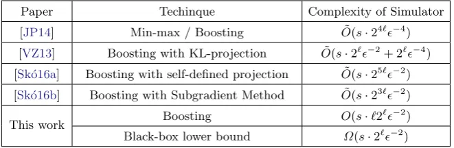
Our Results. In this paper, we achieve the bound ˜O(2`−2) for relative com-plexity, which contains the best components out of three complexity bounds mentioned above. The algorithm we use is also of multiplicative weight update (MWU) method as in [VZ13] but without going through the uniform min-max theorem argument. The additive term 2`−4 in [VZ13] is due to the precision issue when performing multiplication of “real numbers”. The saving of the addi-tive term is based on the observation mentioned in [VZ13] – the KL-projection step in their MWU algorithm is not needed when proving the Leakage Simula-tion Lemma. Thus we can potentially simplify the circuit construcSimula-tion. Indeed, we prove that certain level of truncation on weights does not effect the accuracy too much but helps us reducing the circuit complexity. In table 1, we list out and compare all previous results to ours.
Paper Techinque Complexity of Simulator [JP14] Min-max / Boosting O˜(s·24`−4) [VZ13] Boosting with KL-projection O˜(s·2`−2+ 2`−4) [Sk´o16a] Boosting with self-defined projection O˜(s·25`−2) [Sk´o16b] Boosting with Subgradient Method O˜(s·23`−2)
This work Boosting O(s·`2
`−2) Black-box lower bound Ω(s·2`−2)
Table 1.Summary of exisiting upper bound results and our results.
Implication of Our Results As mentioned before, our result yields a proof of better security in leakage-resilient stream-cipher. All previous results suffer from the term−4[JP14,VZ13]5or the 23` multiplicative factor [Sk´o16b] in the com-plexity bound. In particular, Sk´orski’s gave legitimate examples [Sk´o16a] where the bounds in [JP14] and [VZ13] only guarantee trivial security bounds whenis set to be 2−40. On the other hand, the factor 23` (or even 25`) is significant and makes the guaranteed security bound trivial when the leakage is more than few bits. Therefore, in some reasonable parameter settings, our bound is the only one that can achieve a useful security. Here is a concrete example. If we cons-dier the stream cipher in [JP14] and follow the settings in [Sk´o16a, Section 1.6]: The underlying weak PRF has 256 bits security, the target cipher security is 0 = 2−40 and the round is 16. If the leakage isλ= 17 per rounds, then using our bound, we can guarantee the security against 250-size circuit but all the analyses in [JP14,VZ13,Sk´o16a] guarantee nothing.
5
1.2 Lower Bound Results
Our Results. We show that the simulator must have a “relative complexity” Ω(2`−2) to the distinguisher family by establishing a black-box lower bound, where a simulator can only use the distinguishers in a black-box way. Our lower bound requires an additional mild assumption that the simulator on a given inputx, does not make a query anx06=xto distinguishers.6Querying at points
different from the input seems not helpful, but that makes the behaviors on different inputs not completely independent, which causes a problem in analysis. Indeed, all the known upper bound algorithms (including the one in this work) satisfy the assumptions we made. Still, we leave it as an open problem to close this gap completely.
Comparison to Related Results. In [JP14], they proved a Ω(2`) lower bound for relative complexity under a hardness assumption for one-way functions. Be-sides, there are also lower bound results on the theorems that implied by the Leakage Simulation Lemma, including Regularity Lemma [TTV09], Hardcore Lemma [LTW11], Dense Model Theorem [Zha11], Leakage Chain Rule [PS16] and Hardness Amplification [SV10,AS11]. The best lower bound one can ob-tain before this work isΩ(−2) (from [LTW11,SV10,Zha11]) orΩ(2`−1) (from [PS16]). Thus our lower bound is the first tight lower boundΩ(2`−2) for Leakage Simulation Lemma. See Section4.2for more detailed comparison.
Proof Overview We define an oracle and a joint distribution (X, Z)∈ {0,1}n× {0,1}`. Considering a family of the distinguishers that each of them makes a single query to the oracle, the simulator has to query the oracle at leastΩ(2`−2) times to fool all the distinguishers in the family. Therefore, if the only way to access the oracle is through the distinguishers, the simulator must use at least Ω(2`−2) distinguishers.
We can treat Z as a randomized function of X. That is, if can define g : {0,1}n → {0,1}` such that Pr[g(x) = z] = Pr[Z = z|X = x], then (X, Z) = (X, g(X)). The distribution we consider is that the functiong is deterministic, but the images are “hidden” from the simulator. Note that it is impossible for a simulator to hardwire all 2n images. If the oracle receives a query (x, z) ∈ {0,1}n× {0,1}` withz =g(x), it returns an answer based on the distribution Bern(1/2 +). Otherwise, use the distribution Bern(1/2). Intuitively, the goal of the simulator is to findg(x) for a given inputx. For eachz, due to the anti-concentration bound, it has to make Ω(−2) many queries to check ifg(x) =z. And if it has to check a constant fraction of allz∈ {0,1}n, then the total query complexity isΩ(2`−2).
2
Preliminaries
2.1 Basic Definitions
Notations. For a natural number n, [n] denotes the set {1,2, . . . , n} and Un denotes the uniform distribution over{0,1}n. For a finite setX,|X |denotes its cardinality, andUX denotes the uniform distribution overX. For a distribution
X overX,x←X meansxis a random sample drawn fromX. Bern(p) denotes the Bernoulli distribution with parameter 0≤p≤1. For any function f, ˜O(f) meansO(flogkf) and ˜Ω(f) meansΩ(f /logkf) for some constant k >0.
Definition 1 (Statistical Distance). Let X andY be two random variables. The statistical distance (or total variation) between X andY is denoted as
∆(X, Y) =X x
1 2
Pr [X =x]−Pr [Y =x] .
Also, we say X andY are -closeif∆(X, Y)≤.
Definition 2 (Indistinguishability). Let X, Y be distributions over {0,1}n. We say X and Y are (s, )-indistinguishable if for every circuit f : {0,1}n → {0,1} of sizes,
x←EX[f(x)]−y←EY[f(y)]
≤.
2.2 Multiplicative Weight Update
Consider the following prediction game. In each round, a predictor makes a pre-diction and receive a payoff. There areNexperts that the predictor can refer to. That is, the predictor can (randomly) choose an expert to follow. The goal of the predictor is to minimize total payoff in many rounds. We called the difference between the total payoff of predictor and of the best expertregret, which is the criterion we use to measure the performance of the predictor. The Multiplica-tive weight update (MWU) algorithm provides a good probabilistic strategy for prediction. The overview of the algorithm is as follows. In the first round, the predictor simply chooses an expert uniformly at random. In the following rounds, the predictor updates the probabilities of choosing experts “multiplicatively” ac-cording to their performances in the previous round. The formal algorithm and the guarantees by the MWU algorithm is stated below.
Lemma 1 (Multiplicative weight update [AHK12]).Consider aT-round game such that int-th round, the predictor chooses a distribution Dt over[N], and obtains a payoff according to the functionft: [N]→[0,1]. Let 0< η≤1/2 be an update rate. If player 1 chooses Dt as in Algorithm 1, then for every i∈[N],
T X
t=1 E j←Dt
[ft(j)]≤ T X
t=1
In particular, if we setη=plogN/T, we have T
X
t=1 E j←Dt
[ft(j)]≤ T X
t=1
ft(i) +OpTlogN
Algorithm 1: Multiplicative weight update
1 For alli∈[N] setwi:= 1.
2 fort:= 1 toT do
3 ChooseDt such thatDt(i)∝wi.
4 fori:= 1toN do
5 wi:=wi·(1−η)ft(i);
As the regret grows sub-linearly to T, the predictor can achieve δ average regret whenT is large enough.
Corollary 1. There existsT =O ln2N
such that for alli∈[N], 1
T X
t E j←Dt
[ft(j)]≤ 1 T
X
t
ft(i) +.
Freund and Schapire discovered the connection between MWU algorithm and zero sum game [FS96] by treating the best response of Player 2 as the payoff function. MWU algorithm not only gives a new proof of von Neumanns Min-Max Theorem, but also provides a way to “approximate” the universal strategy obtained by the Min-Max Theorem7.
Lemma 2 ([FS96]).Consider a zero-sum game between Player 1 and Player 2 whose (pure) strategy spaces areP andQ, respectively, and|P|=N. The payoff to Player 2 is defined by the function u: P × Q → [0,1]. We apply the MWU algorithm (Algorithm 1) in the following way to get the mixed strategy P∗ and Q∗.
1. Treat each pure strategy in|P|as an expert. LetPtdenote the mixed strategy described byDt (thei-th pure strategy is chosen with probabilityDt(i)). 2. LetQt denote the best response of Player 2 toPt. Namely
Qt= min
Q p←PEt,q←Q
f(p, q)
3. Set the payoff function in the MWU algorithm asft(·) =M(·, Qt). 4. LetP∗= 1
T P
tPtandQ∗= T1 PtQt. 7
If we conduct the above procedure forT =O(logN/2)rounds, the mixed strate-gies P∗, Q∗ are almost the equilibrium strategies. That is
max
q p←EP∗[u(p, q)]−≤maxQ minP p←P,qE←Q[u(p, q)] = min
P maxQ p←P,qE←Q[u(p, q)]≤minp q←EQ∗[u(p, q)] +.
3
Simulating Auxiliary Inputs
The formal description of Leakage Simulation Lemma with our improved pa-rameters is as follows.
Theorem 2 (Leakage Simulation Lemma). Let n, `∈ N, > 0 andF be a collection of deterministic distinguishers f : {0,1}n× {0,1}` → {0,1}. For every distribution(X, Z)over {0,1}n× {0,1}`, there exists a simulator circuit h:{0,1}n→ {0,1}` such that
1. hhas complexityO(2˜ `−2)relative toF. i.e.,hcan be computed by an oracle-aided circuit of sizeO(2˜ `−2)with oracle gates are functions in F.
2. (X, Z)and(X, h(X))are indistinguishable byF. That is, for every f ∈ F,
(x,z)←E(X,Z)[f(x, z)]−h,xE←X[f(x, h(x))]
≤.
SetF to be a set of Boolean circuits of size at mosts, we immediate have the following corollary.
Corollary 2. Let s, n, ` ∈ N and > 0. For every distribution (X, Z) over {0,1}n× {0,1}`, there exists a simulator circuit of size s0 = ˜O(s·2`−2) such that (X, Z)and(X, h(X))are (s, )-indistinguishable.
3.1 Boosting
There are numbers of proof of Leakage Simulation Lemma as discussed in the introduction. We focus on the “boosting” type of proof as it usually gives us better circuit complexity. The boosting framework has the following structure:
1. Choose a proper initial simulatorh.
2. If h satisfies the constraint above, return h. Otherwise, find f ∈ F0 which
violates the constraint. 3. Update hwithf and repeat.
may cause negative weights, so they need an extra efforts (Both algorithm-wise and complexity-wise) to fix it. Vadhan and Zheng use multiplicative weight up-date instead [VZ13], which not only avoids the issue above but also converges faster. However, the number of bits to represent weights increases drastically after multiplications, and that causes the O(2`−4) additive term in the com-plexity. Since the backbone of our algorithm is same as in [VZ13], we review their idea first in the next section, and then show how the additive term can be eliminated in Section3.3.
3.2 Simulate Leakage with MWU
In this section, we show how MWU algorithm helps in simulating auxiliary inputs and why we can achieve the low round complexity. It is convenient to think Z as a randomized function ofX. That is, we can defineg:{0,1}n→ {0,1}`such that Pr[g(x) =z] = Pr[Z =z|X =x], then (X, Z) = (X, g(X)). Essentially, the goal is to find an “efficient function”hto simulateg.
Now we show that how the simulation problem problem is related to a zero-sum game, thus can be solved via MWU algorithm. The first step is to remove the one-sided error constraint. Let F0 denote the closure of F under complement,
namely, F0 = {f,1−f : f ∈ F }. Then the indistinguishability constraint is
equivalent to
∀f ∈ F0 , E
h,x←X[f(x, h(x))]−g,xE←X[f(x, g(x))]≤.
Then consider the following zero-sum game: Player 1 choose a simulatorh, Player 2 choose a distinguisherf, and the payoff to Player 2 is
E
h,x←X[f(x, h(x))]−g,xE←X[f(x, g(x))].
One can get a bounded relative complexity ofgby simply applying Lemma2
with treating all functions from{0,1}n to{0,1}`as pure strategies of Player 1. However, relative complexity is O(s·2n`−2) and hence is inefficient. To solve the above issue, Vadhan and Zheng observed that the marginal distribution of X-part is fixed. Thus we can consider the MWU algorithm for every X = x, where in each run of MWU, the Player 1 strategy space is simply a distribution over{0,1}`, hence the round complexity is merely O(`/2).
While the framework Vadhan and Zheng’s considered is more general, the proof is also more complicated. Below we give a simpler proof which only uses the no-regret property of MWU.8Note that any no-regret algorithms for expert
learning will work for this proof. Indeed, by applying online gradient descent instead of MWU we will get an additive boosting simulator. Nevertheless, multi-plicative weight update is optimal in expert learning, which explains why MWU converges faster than additive boosting proofs.
Algorithm 2: Construction of Simulatorh
1 Input:x∈ {0,1}n
2 Parameter: >0
3 LetT =O(n/2),η=plogN/T.
4 For allz∈ {0,1}`, setwx(z) = 1.
5 Leth0 be a randomized function such that Pr [h0(x) =z]∝wx(z).
6 fort = 1→T do
7 Letft∈ F0= arg maxf∈F0Eht−1,x←X[f(x, ht−1(x))]−Eg,x←X[f(x, g(x))].
8 if Eht−1,x←X[f(x, ht−1(x))]−Eg,x←X[f(x, g(x))]≤then
9 Returnht−1(x)as the outputh(x)
10 For allz∈ {0,1}`, setwx(z) =wx(z)·(1−η)ft(x,z)
11 Letht be a randomized function such thatPr [ht(x) =z]∝wx(z).
12 ReturnhT(x)as the outputh(x)
Lemma 3. Let X be a distribution over {0,1}n andg :{0,1}n → {0,1}` be a randomized function. For a given error parameter , the function hdefined by Algorithm2satisfies
∀f ∈ F0 , E
x←X[f(x, h(x))]−x←EX[f(x, g(x))]≤. Proof. For a fixedx, if there existsf ∈ F0 such that
E
h[f(x, h(x))]−Eg[f(x, g(x))]> ,
then the algorithm returns at the line 12. That means for allt∈[T], we have
E ht−1
[ft(x, ht−1(x))]−E
g[ft(x, g(x))]> , (1) and so
1 T
T X
t=1 E ht−1
[ft(x, ht−1(x))]− 1 T
T X
t=1
Eg[ft(x, g(x))]> , (2)
However, by Corollary1, for everyz∈ {0,1}`,
1 T
T X
t=1 E ht−1
[ft(x, ht−1(x))]≤ 1 T
T X
t=1
ft(x, z) +.
By takingzoverg(x), we get a contradiction. Therefore, for allf ∈ F,
E
3.3 Efficient Approximation
Algorithm 2 provides a simulator which fools all distinguishers in F by error up to . However, we have only proved a bound for the number of iterations, but not for the complexity of hT itself. Actually, the circuit complexity of a naive implementation of Algorithm2is not better than using additive boosting. Nevertheless, we will show that there exists an efficient way to implement hT approximately, of which the complexity is not much larger than evaluating the distinguishersT times.
In below, we assume all functions f ∈ F has circuit compleixty at most s. From Algorithm2, we can seehT(x) returnsz with probability proportional to (1−η)Pifi(x,z). A natural way to approximatehT is to compute (1−η)Pifi(x,z)
for each z and apply a rejection sampling. Without loss of generality, we can assume that (1−η) can be represented in O(log1
η) bits, and thus, it takes at most O(klog1η) to represent (1−η)k for k ∈ N. Since Pifi(x, z) is at most T, it takes O(T s+T2log2 1
η) complexity to compute (1−η) P
ifi(x,z) by naive
multiplication, orO(T s+T2logTlog1
η) via lookup table. Therefore there exists an approximation of hT of sizeO((T2log2 1η +T s)·2`), which is ˜O(s·2`−2+ 2`−4)) after expandingT and η. This is the complexity claimed in [VZ13]. As mentioned in [Sk´o16a], the ˜O(2`−4) term may dominate in some settings, so the bound in [VZ13] is not always better.
Now we state the idea of approximating normalized weights efficiently. Ob-serve that weights are of the form (1−η)Pifi(x,z). If the total weight is
guaran-teed to be at least 1, then intuitively, truncating the weight at eachz∈ {0,1}` a little amount does not influence the result distribution too much. Hopefully, if the truncated values can be stored with a small number of bits, a lookup table which maps P
ifi(x, z) to the truncated value of (1−η) P
ifi(x,z) is affordable.
In the lemma below we formalize the above intuition.
Lemma 4. Suppose there are two sequences of positive real numbers{γi}i∈[n], {wi}i∈[n] such that ∀i ∈ [n], γi ≤ wi. Let r = Piγi/
P
iwi and X, X
0 be a
distribution over [n] such that Pr [X =i] ∝ wi and Pr [X0 =i] ∝ (wi−γi), respectively. Then ∆(X, X0)≤ r
1−r. Proof.
∆(X, X0) =1 2 X z wz P
iwi
−Pwz−γz i(wi−γi)
=1 2 X z γzP
iwi−wz P
iγi (P
iwi)2(1−r) ≤1 2 X z
wzPiγi+γzPiwi (P
iwi)2(1−r) =
P
iwiPiγi (P
iwi)2(1−r)
= r
Corollary 3. Let h0:{0,1}n→ {0,1}` be a function which satisfies
Pr[h0(x) =z] = (1−η) P
ifi(x,z)−γ
x,z P
z0 (1−η)
P
ifi(x,z0)−γ
x,z0
where
γx,z ≤min (
(1−η)Pifi(x,z), η
2`(1 +η)· X
z0
(1−η)Pifi(x,z0)
) .
Then for any x∈ X,h0(x) isη-close tohT(x).
By the above corollary, the following procedure gives a good approximation of hT.
1. For everyz∈ {0,1}`, computeAdv(x, z) =P
ifi(x, z)−minz0( P
ifi(x, z
0)).
This can be done by a circuit of sizeO(2`·(sT+TlogT)).
2. Because there isz0such thatAdv(x, z0) = 0, we havePz(1−η)Adv(x,z)≥1. Letk=O(`log(1/δ)) be the smallest integer which satisfies 2−k ≤ 2`(1+η η).
By Corollary3, if we truncate (1−η)Adv(x,z)down to the closest multiple of 2−k, the corresponding distribution is stillη-close toh
T(x). Leth0(x) denote the truncated distribution.
3. Observe that the truncated value is positive only if Adv(x, z) is less than some thresholdt=O(k/η). Therefore we can build a lookup table consists of the truncated value of (1−η)j forj∈[t]. Such table is of sizeO(tlogt·k). With this table we can query truncated value of (1−η)Adv(x,z) for eachz. 4. By rejection sampling, we can sample aη-approximation ofh0(x) in at most
O(2`log(1/δ)) rounds, and each round takes onlyO(k) time.
Leth∗ be the circuit which uses above steps to approximatehT. Sinceη=O() andh(x) is 2η-close tohT(x), we have
E
h,x←X[f(x, h(x))]−g,xE←X[f(x, g(x))]≤+ 2η=O()
for anyf ∈ F0. (Note that we can always rescale to make the final gap is at
most.) Since the complexity of the first step dominates all other steps,his of complexityO(2`·(sT+TlogT)) = ˜O(s·2`−2).
4
Lower Bound for Leakage Simulation
a simulator which makes fewer queries? It might be possible to find a boosting procedure using fewer distinguishers, or maybe we can skip some z ∈ {0,1}` when querying f(x, z) for somef. However, in this section we will show that the MWU approach is almost optimal: anyblack-boxsimulator which satisfies an independence restriction has to makeΩ(2`−2) queries to fool the distinguishers.
4.1 Black-Box Model
To show the optimality of the MWU approach, we consider black-box simulation, which means we only use only the distinguishers as black-box and does not rely on how they are implemented. Note that all known results of leakage simulation ([JP14,Sk´o16a,VZ13]) are black-box. Indeed, all the leakage simulation results are in the following form: first learn a set of distinguishers {f1, . . . , fq0} which
is common for each x, then queryfi(x, z) for each z∈ {0,1}` and i∈[q0], and finally combine them to obtain the distribution ofh(x). The model we consider is more general than this form, so it also rules out some other possible black-box approaches.
Definition 3 (Simulator). Given a function g:{0,1}n → {0,1}`, a distribu-tionX over{0,1}n and a setFof functions{0,1}n+`→ {0,1}, we say function h:{0,1}n→ {0,1}` is an (, X,F)-simulator ofg if
∀f ∈ F ,
g,xE←X[f(x, g(x))]−h,xE←X[f(x, h(x))]
≤.
Definition 4 (Black-Box Simulator). Let `, m, a ∈ N and > 0. We say an oracle-aid simulation circuit D(·) which takes two inputs x ∈ {0,1}n and α ∈ {0,1}a is a black-box (, `, m, a)-simulator with query complexity q if it satisfies the follows. For every function g:{0,1} → {0,1}`, distributionX over {0,1}n and a set of distinguishers F with |F | ≤ m, there exists α ∈ {0,1}a (which we call “advice string”) such thatDF(·, α)is an (, X,F)-simulator for g andD uses at most q oracle gates.
We say a black-box simulator is asame-inputblack-box simulator if for every f ∈ F,D only queriesf(x,·) when computing on input x. We say a black-box simulator is non-adaptiveif the choice of the oracle queries (including the choice of f and query input) does not depend on any response of the oracle.
Remark 1. A reasonable range of parameters are −1,2`,log|F | < 2o(n) since all the simulations we know is of complexity poly(−1,2`,log|F |). Note that when we consider F to be the set of every distinguisher of size at most s, log|F | = O(slogs). Besides, we also assume a = 2o(n) so that the simulator cannot trivially takeαas an expression ofg.
It is not hard to see that all the boosting approaches we mentioned above are in this model: the adviceα is of length O(qlog|F |) and stands for “which distinguishers should be chosen”, and D queries every chosen distinguisher f with input (x, z) for every z ∈ {0,1}` when computing DF,α(x). Moreover, these simulation algorithms are non-adaptive. We can write the MWU approach as the following corollary:
Corollary 4. For every 0 < < 12, `, m ∈ N, there exists an non-adaptive same-input black-box(, `, m, a)-simulator with query complexity q=O(`2`−2) anda= ˜O(qlog|F |).
Besides capturing all known simulators, our lower bound also rules out the adap-tive approaches. Whether there exists a faster simulation not satisfying the same-input restriction is left open, but it is hard to imagine how querying different input is useful.
4.2 Main Theorem and Related Results
Theorem 3. For every 2−o(n) < < 0.001, ` = o(n), ω(2`/3) < m < 22o(n) and a = 2o(n), a same-input black-box (, `, m, a)-simulator must have query complexity q=Ω(2`−2).
Remark 2. Forwe require it to be smaller than some constant so that Bern(1 2+ Θ()) is well defined. Besides, we also require the size of distinguisher setm to be large enough to guarantee that the simulator must “simulate” the function instead of fooling distinguishers one by one. As we saw in Remark1, the range of parameters here is reasonable.
Before this paper, there were some lower bounds either for Leakage Simu-lation Lemma itself or for its implications. We classify these results by their models as follows.
– Non-Adaptive Same-Input Black-Box Lower Bounds. Recall that
Leakage Simulation implies Hardcore Theorem and Dense Model Theorem. Lu, Tsai and Wu [LTW11] proved an Ω(log(1
δ)/
2) lower bound for query complexity in Hardcore Lemma proof where δ denotes the density of the hardcore set. By takingδ=Θ(1) we can obtain anΩ(1/2) lower bound for query complexity of Leakage Simulation. Similarly, Zhang [Zha11] proved a lower bound for query complexity in Dense Model Theorem proof which implies the sameΩ(1/2) lower bound.9Besides, Pietrzak and Sk´orski [PS16]
proved a Ω(2`/) lower bound for leakage chain rule, which also implies a Ω(2`/) lower bound for Leakage Simulation. These lower bounds assume both the non-adaptivity and the independence of inputs.10
9
The box model these results considered is more restricted. Actually, the black-box model in [LTW11] does not contain Holenstein’s proof [Hol05]. Nevertheless, their proof for query lower bound also works for the model we define here.
– Non-Adaptive Black-Box Lower Bounds. Impagliazzo [Imp95] proved that the Hardcore Lemma implies Yao’s XOR Lemma [GNW95,Yao82], which is an important example of hardness amplification. Since the reduction is black-box, it is not hard to see that theΩ(log(1δ)/2) lower bound for hard-ness amplification proved by Shaltiel and Viola [SV10] is also applicable to Hardcore Lemma. Similarly, by setting δ = Θ(1) we get a Ω(1/2) lower bound for Leakage Simulation. Moreover, this lower bound does not require the same-input assumption.11 Nevertheless, the proof highly relies on
non-adaptivity.
– General Black-Box Lower Bounds. Artemenko and Shaltiel [AS11] proved anΩ(1/) lower bound for a simpler type of hardness amplification, and removed the non-adaptivity. Their result implies a general black-box lower bound for Leakage Simulation, but the lower bound is far from optimal.
– Non-Black-Box Lower Bounds. Trevisan, Tulsiani and Vadhan show that the simulator cannot be much more efficient than the distinguish-ers [TTV09, Remark 1.6]. Indeed, for any large enoughs∈Nthey construct a functiong such that any simulatorhof complexityscan be distinguished from g by a distinguisher of size ˜O(ns). Jetchev and Pietrzak [JP14] also show anΩ(2`·s) lower bound under some hardness assumptions for one-way functions.
None of the existing results imply an optimal lower bound for Leakage Sim-ulation. However, proving a lower bound for Leakage Simulation might be a simpler task, and it turns out that we can prove a lower bound of Ω(2`−2). The basic ideas is as follows, and would be further explained in the proof. To capture the 2` factor, for each distinguisherf and inputxwe hide information at f(x, z) for a random z, similar to the proof in [PS16]. Then checking all z over{0,1}`is necessary. Although the claim seems trivial, the analysis would be more complicated in our adaptive model. To capture the −2 factor, we utilize the anti-concentration of almost uniform Bernoulli distribution Bern(12+Θ()), so that Ω(1/2) samples are needed to distinguish it from uniform distribu-tion with constant probability. A similar concept can be found for example in [Fre95,LTW11,PS16]. Note that in [PS16] they only require an advantage of when distinguishing such Bernoulli distribution from uniform, which causes an O(1/) loss in complexity.
4.3 Proof of Theorem 3
Overview We would like to show that there exists a function g and a set of distinguisherF such that any simulator hwith limited queries toF cannot ap-proximategwell. Since|F |is much larger than the number of queries, there exist some distinguishers which can distinguish g and any bad simulator h “fairly”, adaptively chosen input. In this case non-adaptivity causes a 2`additive loss. This can be viewed as an evidence that adaptivity might be useful.
11
i.e. these distinguishers are independent of h. Therefore more queries are re-quired to successfully simulate g and fool F. We will prove the existence of g andF by probabilistic argument.
To make the simulation task as hard as possible, letgbe a random function. Besides, for any distinguisher f ∈ F, let f(x, z) be a random bit drawn from Bern(1
2+c1) for some constantc1ifz=g(x), or from Bern( 1
2) otherwise, so that a query tof provides least possible information.12 To understand such setting,
we can imagine that there exists a random oracleOwhich takes input (x, z) and only return biased bit atz=g(x) for eachx. Theng(x) is considered as thekeyto the oracle, and our goal is to find out the correct key. Eachf ∈ Fcan be viewed as a collection of samples from the oracle with certain randomness. Intuitively, since f(x, g(x)) is only Θ() away from uniform, f can distinguish g and any bad simulator h which does not approximate g with constant probability. To approximate gwell, we need to test all 2` keys to find the correct one. Besides, it requires Ω(1/2) samples to distinguish Bern(1
2 +Θ()) and Bern( 1 2) with constant probability, so Ω(1/2) queries are required for each key to make sure we can distinguish the real key from other fake keys. Therefore a successful simulatorhshould make at leastΩ(−22`) queries.
Now we proceed to the formal proof. Assume for contradiction that D is a black-box (, `, m, a)-simulator with query complexity q ≤ c2(2`−2), where c2= 3600001 . Let g:{0,1}n→ {0,1}` be a random function such that for every x ∈ {0,1}n, g(x) is chosen uniformly at random from {0,1}`. Let F be a set of random function defined in previous paragraph, and we specify thatc1= 30. First we prove that given any fixed advice stringα, the decision functionDF(, α) cannot guessg correctly with high enough probability over the choice ofF and g.
Lemma 5. Fix α and let h=DF,α. For anyx∈ {0,1}n, we have Pr[h(x) = g(x)]≤1− 3
c1, where the probability is taken over the choice ofg(x),f(x,·)for every f ∈ F (abbreviated as F(x)), and the randomness ofh.
Proof. Without loss of generality, assume thathhas no randomness other than oracle queries. (We can obtain the same bound for probabilistichby taking av-erage over deterministic circuits.) We also assume thathalways makeqdifferent queries by adding dummy queries.
Consider has a decision tree where queries are the nodes and different an-swers represent different branches. For every fixedg(x) andF(x), the computa-tion ofh(x) corresponds to a root-to-leaf path denoted ast={a1, . . . , aq}where ai is the answer to the i-th query, and we callt transcript. LetT be a random variable over {0,1}q which represents such transcript. Note that the output of h(x) is uniquely determined by its transcript. LetDec:{0,1}q → {0,1}`denote the corresponding decision function from transcript to output. Then we have
Pr[h(x) =g(x)] = Pr[Dec(T) =g(x)] =X t,k
Pr[T =t, g(x) =k, Dec(t) =k].
To prove the upper bound for Pr[h(x) =g(x)], first we consider an ideal case such that each function in F is an uniform random function. In this case, for every (t, k) ∈ {0,1}q× {0,1}`, Pr[T∗ =t, g(x) = k] = 2−(q+`) where T∗ is the ideal
transcript, i.e., uniform distribution over {0,1}q. Since for each t there exists a uniquek where Dec(t) =k, only 2q pairs (t, k) are correct (i.e. Dec(t) = k). In such ideal case, we have Pr[h∗(x) =g(x)] = 2−` whereh∗ denotes the ideal
variant ofh. In the real case, Pr[T =t, g(x) =k] can be at most 2−`(1 2+c1)
q, in the case that hqueries with correct key in every query and all the responses are 1. However, there does not exist too many extreme cases like this. Besides, we have seen that most of the pairs (t, k) over {0,1}q × {0,1}` do not satisfy Dec(t) =k. Therefore we can expect that a large fraction of pairs are normal (i.e. chosen with probability Θ(2−(q+`))) and wrong (i.e. Dec(t) 6= k). Such statement implies a lower bound for Pr[h(x)6=g(x)].
Next we formally prove the statement above. Consider any transcriptt = {a1, a2, . . . , aq}. Recall that the queries made byhare uniquely determined by t: the first query is fixed, the second query is determined by the first bit oft, and so on. Let{z1, z2, . . . , zq}be the sequence of key such that thei-th query is fi(x, zi) for somefi∈ F. For anyk∈ {0,1}`, t∈ {0,1}q, letui denote the index of the i-th useful query, which means the i-th index satisfying zui = k. Then we define Nb(t, k) = P
i[aui =b] for b ∈ {0,1}, which represents the number
of useful queries with response b. Besides, letN(t, k) =N0(t, k) +N1(t, k) and N∆(t, k) =N0(t, k)−N1(t, k). Similarly, for j≤N(t, k), we define Nb(t, k, j) = Pj
i=1[aui =b] forb∈ {0,1}andN∆(t, k, j) =N0(t, k, j)−N1(t, k, j), which only
consider the first j useful queries. Recall that for anyf ∈ F,f(x, z) is uniform whenz6=g(x) and biased whenz=g(x). For any fixed (t, k),
Pr[g(x) =k, T =t] = 1
2
(`+q−N(t,k))1 2−c1
N0(t,k)1 2+c1
N1(t,k)
=
1 2
(`+q)
(1−2c1)
N∆(t,k) 1−4c2 1
2N1(t,k)
≥
1 2
(`+q)
(1−2c1)
N∆(t,k) 1−4c2 1
2N(t,k)
(3)
Therefore a pair (t, k) is normal ifN∆(t, k) = O(1/) and N(t, k) = O(1/2). We claim that a large enough fraction of pairs over {0,1}q × {0,1}` are wrong and normal as following:
Claim. Letq0= 5q/2`≤5c
2−2. Then for at least 15 fraction of pairs (t, k) over {0,1}q× {0,1}` satisfies the following conditions:
1. Dec(t)6=k. 2. N(t, k)< q0. 3. N∆(t, k)<√5q0.
1. Only 2−` of pairs are correct:
This obviously holds because (t, k) is correct only whenDec(t) =k. 2. At most 15 of pairs (t, k) satisfy N(t, k)≥q0:
For any t we have Ek←U`[N(t, k)] =
q
2`. By Markov’s inequality, at most
q 2`q0 =
1
5 of pairs satisfyN(t, k)≥q
0.
3. For at most 1
10 of pairs (t, k),N(t, k)< q
0 andN
∆(t, k)> √
5q0:
Fixk. LetT∗be a random transcript which is uniform over{0,1}q. Consider a sequence of random variable{Yj} depending onT∗ such that
Yj = (
N∆(T∗, k, j), ifj < N(T∗, k) N∆(T∗, k), otherwise.
It’s not hard to see that{Yi} is a martingale with difference at most 1. By Azuma’s inequality, we have Pr[Yq0 ≥
√
5q0] ≤e−5q0/2q0 <0.1. Since T∗ is
uniform, the statement above is the same as saying for at most 0.1 fraction oft∈ {0,1}q,Y
q0(t)≥
√
5q0. When restricted tot satisfyingN(t, k)< q0 we
haveN∆(t, k) =Yq0(t)≥
√ 5q0.
By union bound, all three conditions in the claim hold simultaneously for at least 15 of pairs over{0,1}q× {0,1}`.
Now consider any pair (t, k) which satisfies condition 2 and 3 in the claim above, in other word a normal pair. By inequality (3), we have
Pr[g(x) =k, T =t]≥(1/2)(`+q)(1−2c1)N∆(t,k)(1−4c212)N(t,k) ≥(1/2)(`+q)(1−2c1)
√
5q0
(1−4c212)q0 (4) = (1/2)(`+q)(1−2c1)5
√
c2−1(1−4c2 1
2)5c2−2 ≥(1/2)(`+q)(0.3)10c1
√
c2(0.3)20c21c2 (5)
≥(1/2)(`+q)·0.5 (6)
The inequality (5) holds because (1−δ)1/δ ≥0.3 for any 0 < δ ≤0.1. Since 1 5 of pairs satisfy the conditions above, we have
Pr[h(x)6=g(x)] =X k,t
[g(x) =k, T =t, Dec(t)6=k]≥0.1. (7)
Therefore Pr[h(x) =g(x)]≤0.9 = 1− 3 c1.
coincident with queries inhwith probability mq. Even in the worst case thatfR returns 1 in all these cases, we still have
E[fR(x, g(x))]≤ 1
2 + Pr[g(x) =h(x)]·c1+ q
m (8)
≤ 1
2 + (c1−2) (9)
becausemis large enough. Also we haveE[fR(x, g(x))] = 12+c1by definition. Therefore, E[fR(x, g(x))−fR(x, h(x))] ≥ 2. Let X be the uniform distribu-tion. Note that for differentx, g(x) andF(x) are chosen independently. There-fore Eh[fR(x, g(x))−fR(x, h(x))]13 for each x are independent random vari-ables since it is only influenced by randomness of g(x) andF(x). By Chernoff-Hoeffding bound, Ex←X[fR(x, g(x))−fR(x, h(x))] < holds with probability 2−Ω(22n)
over the choice ofF andg. By taking union bound overα, we have
∀α∈ {0,1}2o(n) , E
x←X
fR(x, g(x))−fR(x, DF(x, α))
≤ (10)
with probability 2−Ω(22n)+2o(n), which is less than 1 for large enoughn. By the probabilistic argument there exists a functiong and a setF such that
E
x←X[fR(x, g(x))−fR(x, D
F(x, α))]> . (11)
By averaging argument, for anyα, there existsf ∈ Fsuch thatf can distinguish (X, DF(X, α)) and (X, g(X)). Therefore the simulation fails no matter whatα is, which contradicts to our assumption. Thus there is no simulator with query complexityc2(2`−2).
To summarize, we proved anΩ(2`−2) lower bound for black-box (, `, k, a)-simulator, while the upper bound is onlyO(`2`−2). Note that in order to apply Chernoff bound, we need the same-input assumption (i.e. D(x) cannot query F(x0) for x0 6= x) to guarantee the independence of different x, even though
querying with different input seems useless. A general black-box tight lower bound is left for future work.
References
AHK12. Sanjeev Arora, Elad Hazan, and Satyen Kale. The multiplicative weights update method: a meta-algorithm and applications. Theory of Computing, 8(1):121–164, 2012.
AS11. Sergei Artemenko and Ronen Shaltiel. Lower bounds on the query complex-ity of non-uniform and adaptive reductions showing hardness amplification. In Leslie Ann Goldberg, Klaus Jansen, R. Ravi, and Jos´e D. P. Rolim, editors,Approximation, Randomization, and Combinatorial Optimization. Algorithms and Techniques - 14th International Workshop, APPROX 2011,
and 15th International Workshop, RANDOM 2011, Princeton, NJ, USA, August 17-19, 2011. Proceedings, volume 6845 ofLecture Notes in Computer Science, pages 377–388. Springer, 2011.
CLP15. Kai-Min Chung, Edward Lui, and Rafael Pass. From weak to strong zero-knowledge and applications. In Yevgeniy Dodis and Jesper Buus Nielsen, editors,Theory of Cryptography - 12th Theory of Cryptography Conference, TCC 2015, Warsaw, Poland, March 23-25, 2015, Proceedings, Part I, vol-ume 9014 of Lecture Notes in Computer Science, pages 66–92. Springer, 2015.
DBL08. 49th Annual IEEE Symposium on Foundations of Computer Science, FOCS 2008, October 25-28, 2008, Philadelphia, PA, USA. IEEE Computer Society, 2008.
DP08. Stefan Dziembowski and Krzysztof Pietrzak. Leakage-resilient cryptography. In 49th Annual IEEE Symposium on Foundations of Computer Science, FOCS 2008, October 25-28, 2008, Philadelphia, PA, USA[DBL08], pages 293–302.
FK99. Alan M. Frieze and Ravi Kannan. Quick approximation to matrices and applications. Combinatorica, 19(2):175–220, 1999.
Fre95. Yoav Freund. Boosting a weak learning algorithm by majority.Inf. Comput., 121(2):256–285, 1995.
FS96. Yoav Freund and Robert E. Schapire. Game theory, on-line prediction and boosting. In Avrim Blum and Michael Kearns, editors,Proceedings of the Ninth Annual Conference on Computational Learning Theory, COLT 1996, Desenzano del Garda, Italy, June 28-July 1, 1996., pages 325–332. ACM, 1996.
GNW95. Oded Goldreich, Noam Nisan, and Avi Wigderson. On yao’s xor-lemma. Electronic Colloquium on Computational Complexity (ECCC), 2(50), 1995. GW11. Craig Gentry and Daniel Wichs. Separating succinct non-interactive ar-guments from all falsifiable assumptions. In Lance Fortnow and Salil P. Vadhan, editors, Proceedings of the 43rd ACM Symposium on Theory of Computing, STOC 2011, San Jose, CA, USA, 6-8 June 2011, pages 99– 108. ACM, 2011.
HILL99. Johan H˚astad, Russell Impagliazzo, Leonid A. Levin, and Michael Luby. A pseudorandom generator from any one-way function. SIAM J. Comput., 28(4):1364–1396, 1999.
Hol05. Thomas Holenstein. Key agreement from weak bit agreement. In Harold N. Gabow and Ronald Fagin, editors, Proceedings of the 37th Annual ACM Symposium on Theory of Computing, Baltimore, MD, USA, May 22-24, 2005, pages 664–673. ACM, 2005.
HS16. Martin Hirt and Adam D. Smith, editors.Theory of Cryptography - 14th In-ternational Conference, TCC 2016-B, Beijing, China, October 31 - Novem-ber 3, 2016, Proceedings, Part I, volume 9985 ofLecture Notes in Computer Science, 2016.
Imp95. Russell Impagliazzo. Hard-core distributions for somewhat hard problems. In36th Annual Symposium on Foundations of Computer Science, Milwau-kee, Wisconsin, 23-25 October 1995, pages 538–545. IEEE Computer Soci-ety, 1995.
Proceedings, volume 8349 ofLecture Notes in Computer Science, pages 566– 590. Springer, 2014.
LTW11. Chi-Jen Lu, Shi-Chun Tsai, and Hsin-Lung Wu. Complexity of hard-core set proofs. Computational Complexity, 20(1):145–171, 2011.
PS16. Krzysztof Pietrzak and Maciej Sk´orski. Pseudoentropy: Lower-bounds for chain rules and transformations. In Hirt and Smith [HS16], pages 183–203. Rou16. Tim Roughgarden. No-Regret Dynamics, pages 230–246. Cambridge
Uni-versity Press, 2016.
RTTV08. Omer Reingold, Luca Trevisan, Madhur Tulsiani, and Salil P. Vadhan. Dense subsets of pseudorandom sets. In49th Annual IEEE Symposium on Founda-tions of Computer Science, FOCS 2008, October 25-28, 2008, Philadelphia, PA, USA[DBL08], pages 76–85.
Sk´o16a. Maciej Sk´orski. Simulating auxiliary inputs, revisited. In Hirt and Smith [HS16], pages 159–179.
Sk´o16b. Maciej Sk´orski. A subgradient algorithm for computational distances and applications to cryptography. IACR Cryptology ePrint Archive, 2016:158, 2016.
SV10. Ronen Shaltiel and Emanuele Viola. Hardness amplification proofs require majority.SIAM J. Comput., 39(7):3122–3154, 2010.
TTV09. Luca Trevisan, Madhur Tulsiani, and Salil P. Vadhan. Regularity, boosting, and efficiently simulating every high-entropy distribution. In Proceedings of the 24th Annual IEEE Conference on Computational Complexity, CCC 2009, Paris, France, 15-18 July 2009, pages 126–136. IEEE Computer So-ciety, 2009.
VZ13. Salil P. Vadhan and Colin Jia Zheng. A uniform min-max theorem with applications in cryptography. In Ran Canetti and Juan A. Garay, editors, Advances in Cryptology - CRYPTO 2013 - 33rd Annual Cryptology Confer-ence, Santa Barbara, CA, USA, August 18-22, 2013. Proceedings, Part I, volume 8042 ofLecture Notes in Computer Science, pages 93–110. Springer, 2013.
Yao82. Andrew Chi-Chih Yao. Theory and applications of trapdoor functions (ex-tended abstract). In23rd Annual Symposium on Foundations of Computer Science, Chicago, Illinois, USA, 3-5 November 1982, pages 80–91. IEEE Computer Society, 1982.