INTERFERENCE MITIGATION IN
COLOCATED WIRELESS SYSTEMS
Shabbir Ahmed
B.Sc. in Computer ScienceSchool of Engineering and Science
Faculty of Health, Engineering and Science
Victoria University
SUBMITTED IN FULFILLMENT OF THE REQUIREMENTS FOR THE DEGREE OF
DOCTOR OF PHILOSOPHY
I, Shabbir Ahmed, declare that the PhD thesis entitled INTERFERENCE
MITIGATION IN COLOCATED WIRELESS SYSTEMS is no more than 100,000
words in length including quotes and exclusive of tables, figures, appendices,
bibli-ography, references and footnotes. This thesis contains no material that has been
submitted previously, in whole or in part, for the award of any other academic
degree or diploma. Except where otherwise indicated, this thesis is my own work.
Shabbir Ahmed
Abstract
The placement of base station transceivers at close proximity to one another is a
major challenge for RF engineers. In a colocated setting, the base station receivers
have to receive weak desired signals in the presence of high-power transmit/jamming
signals from colocated base station transmitters; resulting in major interference
issues. The thesis identifies two major mechanism of interference for the colocated
victim receiver. First, the strong jamming signals mix within the victim receiver
front-end to produce intermodulation products that may fall on its desired receive
channel and cause interference. The strong signals may also saturate the receiver
circuits and cause desensitization. Second, large jamming signals from one colocated
transmitter can radiate into the antenna system of a second colocated transmitter.
The signals enter the second transmitter in the reverse direction and mix in the
output stage of its power amplifier to produce intermodulation products. These
‘reverse’ intermodulation products get radiated from the antenna system and may
fall on the victim receiver’s desired channel.
The thesis proposes a reference antenna based adaptive cancellation system that
reduces the jammers before they hit the victim receiver’s front-end circuits, thus,
mitigating intermodulation distortions and desensitization. The practicality of the
system is analyzed. Practical measurements show an increased third-order intercept
point (IP3) performance, implying a higher tolerance to jamming signals. This
ben-efit comes at the expense of reduced sensitivity. The IP3 and noise figure expressions
derived for the overall system reveals that the cancellation coupler in the reference
a novel signal-to-interference-and-noise (SINR) analysis is performed to find the
op-timum coupler value that maximizes the system SINR performance. A hardware
prototype achieved a 42dB SINR improvement over a system without the canceling
circuit. It managed 46dB cancellation of jammers in a controlled environment and
25dB in a realistic over-the-air setup. The jammer cancellations were enough to
remove any distortions generated within the victim receiver.
Jammer reduction at the victim receiver does not mitigate the reverse
intermod-ulation products that are radiated from the output of the colocated transmitters.
Hence, the thesis proposes an architecture that regenerates an estimate of the reverse
intermodulation products using the fundamental jammer components and mitigates
them in a postdistortion cancellation circuit. The cancellation is done in baseband
using digital signal processing techniques. A disadvantage is the wide bandwidth
and high sampling rates required to receive both jammers and the corrupt desired
signal in a single unit, particularly when the jammers are well out-of-band. A novel
multiple-front-end receiver architecture is developed to overcome the high sample
rate issue. However, this leads to a frequency offset problem in the regenerated
distortion estimate. A frequency offset correction technique to mitigate the
off-set is incorporated within the distortion regeneration circuit. This novel technique
uses signal correlation to align the frequency, phase and amplitude of the
distor-tion estimate with the interfering reverse intermoduladistor-tion product. Simuladistor-tions and
theoretical analysis are performed to characterize the postdistortion cancellation
system. A prototype of the cancellation system demonstrates 16dB reduction of the
Acknowledgments
First and foremost, I thank Allah (SWT) for giving me the strength, knowledge and
ability to complete this thesis.
I am highly grateful and indebted to my supervisor, Prof. Mike Faulkner, for
his unreserved guidance and support during the whole period of my candidature.
His kindness, patience and encouragement helped me to develop as a competent
researcher. This thesis would not have been possible without his research expertise
and in-depth knowledge. My sincere gratitude to Dr. Stephen Collins, Lance Linton,
Dr. Phillip Conder, Prof. Aladin Zayegh and Prof. Akhtar Kalam for their help
and guidance.
I am most grateful to Dr. Lesley Birch, Elizabeth Smith, Sue Davies and
Shukonya Benka for their continuous support over the last four years. I want to
thank Victoria University for giving me the opportunity to undertake postgraduate
studies here in Australia.
I want to acknowledge all my past and present colleagues in the
telecommunica-tion and microelectronics group who have always helped and encouraged me with
my work, in particular, Waqas, Robab, Rahele, Shahryar, Faizan, Rizwan, Zaheer,
Reza, Vandana, Micheal, Hojjat, Asyik, Hadi, Baharuddin and Andrew. A special
thanks to my friend Mustafa and his family for their kind support.
Last but not the least, my deepest gratitude to my parents, two brothers, sister,
and my wife for their love and support. I am ever indebted to my wife for putting
Doctor of Philosophy Declaration v
Abstract vii
Acknowledgments ix
Contents x
List of Figures xiv
List of Abbreviations xviii
List of Symbols and Variables xx
1 Introduction 1
1.1 Colocation . . . 1
1.2 Interference Issues . . . 3
1.3 Research Goals . . . 5
1.4 Research Contributions . . . 5
1.5 Organization of thesis . . . 6
2 Basic Concepts 8 2.1 Noise and Noise Factor . . . 9
2.2 RF Attenuators . . . 10
2.3 Couplers . . . 10
2.4.1 Harmonic Distortion . . . 12
2.4.2 Intermodulation Distortion . . . 12
2.4.3 1-dB Compression Point (P1dB) . . . 14
2.4.4 Third-order Intercept Point (IP3) . . . 15
2.4.5 Bandwidth Expansion . . . 18
2.5 Practical Measurements . . . 18
2.5.1 Reverse IM3 . . . 19
2.5.2 Desensitization/Blocking . . . 21
2.6 Summary . . . 22
3 Literature Review 23 3.1 Filtering Solutions . . . 24
3.1.1 Knowledge-based Filtering . . . 24
3.1.2 Passive Filtering . . . 25
3.2 Adaptive Cancellation for Forward IM . . . 25
3.2.1 Single Loop Narrowband Cancellation . . . 26
3.2.2 Single Loop Wideband Cancellation . . . 27
3.2.3 Multiple-loop Multi-band Cancellation . . . 27
3.3 The Proposed Solution for Forward IM . . . 29
3.4 Adaptive Cancellation for Reverse IM . . . 30
3.4.1 Transmitter-end Solutions . . . 30
3.4.2 Interference Cancellation Using Regenerated Distortions . . . 31
3.4.2.1 Analog Second-order Postdistortion . . . 32
3.4.2.2 Analog Third-order Postdistortion . . . 32
3.4.2.3 Hybrid Analog and Digital Polynomial Postdistortion 33 3.4.2.4 Digital Polynomial Postdistortion . . . 34
3.5 The Proposed Solution for Reverse IM . . . 34
3.6 Summary . . . 36
4.2 Dynamic Range of the Proposed System . . . 39
4.2.1 Third-order Intercept Point (IP3) . . . 39
4.2.2 Noise Analysis . . . 41
4.2.3 Discussion . . . 43
4.3 Experimental Results . . . 43
4.4 Summary . . . 46
5 Optimized Interference Cancellation 47 5.1 Derivation of SINR . . . 48
5.1.1 Third-order Intermodulation Distortion at the Receiver . . . . 50
5.1.2 Signal and Noise at the Receiver . . . 51
5.1.3 Signal to Interference and Noise Ratio . . . 51
5.2 Optimum Coupling . . . 52
5.3 Hardware Setup and Convergence . . . 54
5.4 Results . . . 57
5.5 Summary . . . 60
6 An Over-the-air Adaptive Cancellation Prototype 62 6.1 Desired Signal Sample in the Reference Input . . . 62
6.2 Experiment Results . . . 65
6.3 Summary . . . 68
7 Postdistortion Cancellation System for Reverse IM Products 70 7.1 Reverse Intermodulation Products . . . 72
7.2 Proposed Architecture and Digital Signal Processing . . . 74
7.2.1 Multiple Receivers . . . 76
7.2.2 Nonlinear Polynomial Function: Cuber . . . 78
7.2.3 Coarse Frequency Correction . . . 79
7.2.4 Fine Frequency Correction . . . 80
7.2.5 Gain-Phase Correction . . . 81
7.3 Simulations and Analysis . . . 82
7.3.1 Buffer/Data Processing Block Size N . . . 82
7.3.2 Fine Frequency Correction . . . 86
7.3.3 Improved Feedback Fine Frequency Correction . . . 87
7.3.4 Coarse Frequency Correction . . . 90
7.4 Practical Measurements . . . 91
7.5 Summary . . . 96
8 Conclusion 98 8.1 Future Work . . . 100
8.1.1 Multi-loop Adaptive Cancellation . . . 100
8.1.2 Cognitive Sensing and Jammer Selection . . . 101
A The Modulation Parameter Factor η 102
B The Variance of fˆF ine
k due to Frequency Offset 104
1.1 Colocation of six base stations on one roof top. Birmingham, UK. . . 2
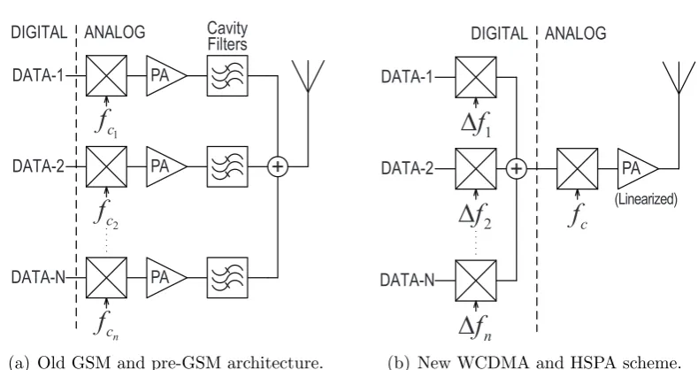
1.2 Multiplexing of base station transmit signals. fc,fc1, fc2, andfcn are carrier frequencies; ∆f1, ∆f2, and ∆fn are frequency offsets from fc. . 3
1.3 Forward and reverse IM products. . . 4
2.1 Noise within a radio system component. . . 9
2.2 Cascaded system components (Noise factor). . . 9
2.3 A directional coupler. . . 10
2.4 Even and odd-order intermodulation products along with the funda-mentals, harmonics and DC [12]. . . 13
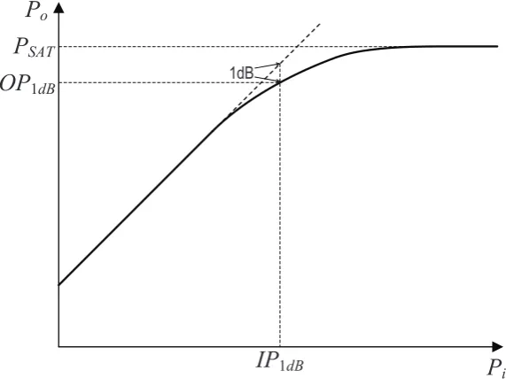
2.5 1dB compression point. . . 14
2.6 Third-order intermodulation distortion causing interference in the de-sired channel of a receiver [6]. . . 15
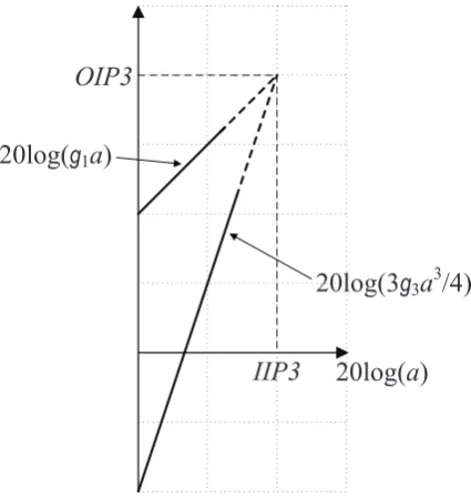
2.7 Two-tone test results for IP3 measurement. . . 17
2.8 Cascaded system components (IP3). . . 17
2.9 Third-order intermodulation distortion causing interference in the de-sired channel of a receiver. . . 18
2.10 Reverse IM3. . . 19
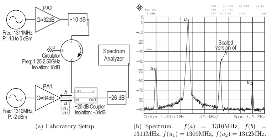
2.11 Reverse IM3 Experiment. . . 20
2.12 Characterization of the reverse IM distortions. . . 21
3.1 Passive pre and post filtering to mitigate colocated interference issues
[17]. . . 25
3.2 Transmitter leakage cancellation for a colocated GPS receiver [22]. . . 26
3.3 Interference cancellation unit for colocated radios [24]. . . 27
3.4 A double loop cancellation adaptive duplexer [25]. . . 28
3.5 The adaptive noise canceling concept [26]. . . 29
3.6 Reverse IM cancellation system using direct feed phasing [28]. . . 31
3.7 Analog second-order postdistortion [35]. . . 32
3.8 Analog third-order postdistortion [36]. . . 32
3.9 Hybrid analog and digital polynomial postdistortion [37] . . . 33
3.10 Digital polynomial postdistortion [38]. . . 34
3.11 Proposed reverse IM postdistortion solution. . . 35
4.1 Proposed adaptive cancellation system for colocated transceivers. . . 38
4.2 IP3 analysis of the proposed system. . . 40
4.3 Noise analysis of the proposed system. . . 42
4.4 Two-tone test on a receiver LNA with 19dB gain and 6dBm input IP3. 44 4.5 Laboratory setup for IP3 and noise measurements. . . 44
4.6 Spectrum of the receiver with and without the proposed cancellation system (using −10dB coupler) during a two-tone test with an input power of −5dBm. . . 45
5.1 An adaptive cancellation system. . . 48
5.2 Signal-to-interference-and-noise analysis. . . 49
5.3 Optimum coupler Copt as a function of jammer X and the Λ value (Λ is primarily a function of the dynamic range of the components in the reference path). . . 53
5.5 Learning curve of the adaptive cancellation system during a two-tone
test with an input power of -10dBm. . . 56
5.6 Spectrum at the receiver with and without the proposed cancella-tion system during a two-tone test with an input power of −10dBm; the fundamentals are at 919.75MHz and 920.25MHz, and the IM3 products are at 919.25MHz and 920.75MHz respectively. The desired signal is not included. . . 57
5.7 SINR vs jammer with different couplers. Noise bandwidth, BW = 5MHz. . . 58
6.1 The proposed adaptive cancellation system. . . 63
6.2 Experimental setup. . . 65
6.3 Signals, as seen by the victim receiver. Signal constellation scatter plots (LHS) and GNU radio spectrum plots (RHS). The GNU radio spectrum plots show relative scales with 75dB representing -39dBm, and on the frequency scale 0 representing 920MHz. . . 67
7.1 Colocated base station transceivers. . . 72
7.2 Proposed DSP. . . 75
7.3 SIRo vs (N/OSR). . . 84
7.4 The effect of frequency offset fF ine on the output SIR. 1bin=f s/N Hz. ‘*’s represent theoretical results. . . 85
7.5 Performance with feedforward fine frequency correction. ‘*’s repre-sent theoretical results. . . 87
7.6 Proposed feedback fine frequency correction. . . 88
7.7 Performance with feedback fine frequency correction. . . 89
7.8 Frequency drift tracking by ˆfF ine k . . . 89
7.9 Probability of acceptable coarse frequency correction (∆f − 0.25fs/N ≤ fCoarse ≤ ∆f + 0.25fs/N) for M = 2N, M = 8N, M = 16N and M = 32N. . . 90
7.11 Frequency spectrum of the jammers and the IM3 product of concern. 93
7.12 Experiment results. Signal constellation scatter plots (LHS) and
frequency spectrum plots (RHS). The spectrum plots show relative
scales with 20dB representing -75dBm. . . 94
7.13 Frequency spectrum of the jammers. . . 95
7.14 Fine frequency tracking by ˆfF ine
ADC Analog-to-Digital Converter
DAC Digital-to-Analog Converter
DC Direct Current
DSP Digital Signal Processing
FDD Frequency Division Duplex
FFT Fast Fourier Transform
FIR Finite Impulse Response
GPA Gain-Phase Adjuster
GPS Global Positioning System
GSM Global System for Mobile Communications
HSPA High Speed Packet Access
IF Intermediate Frequency
IM Intermodulation
IM2 Second-order Intermodulation
IM3 Third-order Intermodulation
IP3 Third-order Intercept Point
ISM Industrial, Scientific and Medical
LHS Left Hand Side
LMS Least Mean Square
LNA Low Noise Amplifier
LO Local Oscillator
MAC Medium Access Control
P1dB 1-dB Compression Point
PA Power Amplifier
QAM Quadrature Amplitude Modulation
QPSK Quadrature Phase Shift Keying
RF Radio Frequency
RHS Right Hand Side
SAW Surface Acoustic Wave
SDR Software Defined Radio
SINR Signal-to-Interference-and-Noise Ratio
SIR Signal-to-Interference Ratio
UE User Equipment
UHF Ultra High Frequency
USRP Universal Software Radio Peripheral
VHF Very High Frequency
WCDMA Wideband Code Division Multiple Access
(·)∗ Complex conjugate
(·)A Signals radiated from jammer A
(·)B Signals radiated from jammer B
(·)D Signals radiated from remote terminal D
(·)H Conjugate transpose
(·)k k-th block of samples
(·)r RF signals
γ Primary to reference SIR voltage ratio Γ Primary to reference SIR power ratio
δM FFT frequency resolution
∆f Total frequency offset (coarse + fine) ∆f1, ∆f2, ... ∆fn Frequency offsets from fc
ε Error signal
η Modulation parameter factor
θ Linear phase across an averaging block Λ A function of GPA dynamic range properties
ρ gain-phase correction factor ˆ
ρ gain-phase correction factor estimate
σ2
(·) Variance of a signal
ϕk Correlation between estimate uˆ′k and primary reception yk Φ(l) FFT of estimate ˆu correlated with primary reception y
1b Through path coupler 1
2b Through path coupler 2
a Complex envelope of jammer A arg(·)/̸ (·) Phase of a complex value
Amp Amplifier
b Complex envelope of jammer B
BW Noise bandwidth
C Coupling gain of the cancellation coupler (Coupler 1)
Copt Optimum coupling value
C ALG FFT frequency correction algorithm
CF Energy cost function at sampling coupler (Coupler 2)
d1 Distance between reference antenna and jammer antenna
d2 Distance between primary antenna and jammer antenna
E{·} Mathematical expectation
fa Carrier frequency of jammer A
fb Carrier frequency of jammer B
fc, fc1, fc2, ... fcn Carrier frequencies
fCoarse Coarse frequency offset
fd Carrier frequency of desired signal
fF ine Fine frequency offset ˆ
fF ine Fine frequency offset estimate
fs Sampling frequency of SDRs
fu, fv Carrier frequencies of reverse IM distortions
F, Fa, Fb, Fc Noise factors of radio components
FA Amplifier noise factor
FL Attenuator noise factor
FRX Receiver noise factor
FT Effective noise factor
FV Vector modulator noise factor
g1 Non-linear system voltage gain
g2 Non-linear system quadratic distortion coefficient
g3 Non-linear system cubic distortion coefficient
gA
3 Jammer A’s power amplifier cubic distortion coefficient
gB3 Jammer B’s power amplifier cubic distortion coefficient
gREF Reference path scaling coefficient
G, Ga, Gb, Gc Gains of radio components
GA Amplifier gain
GCAN Cancellation gain
GCP L2 Coupler 2 through path gain
Ge GPA effective gain
GL Attenuator gain
GRX Receiver gain
GT Total system gain
GV Vector modulator gain
ha,hAu,hb,hBu,hba,hab,hd Channel gains
H Jammer’s gain on the ref. ant. w.r.t. the pri. ant.
ISY S IM3 distortion/interference at receiver output
IP1dB Input P1db power
IIP3 Input IP3 power
IIP3a,IIP3b,IIP3c Input IP3 powers of radio components
IP3A Amplifier input IP3
IP3RX/IIP3RX Receiver input IP3
IP3T Effective input IP3
IP3V Vector modulator input IP3
kB Boltzmann’s constant
lmax Highest power bin in the M-point FFT
L Attenuator
M FFT length
Ns Number of uncorrelated samples in an averaging block
NT/ NSY S Total noise at receiver front-end
N {·} Natural distribution
ok Signal at canceler output
OIP3 Output IP3 power
OIP3A Amplifier output IP3
OIP3e GPA effective output IP3
OP1dB Output P1db power
OSR Over-sampling rate of the desired signal
PSAT Saturated power output
r Received signal at RX input Re[·] Real part of a complex signal
RMSE(·) Root mean square error
RX Victim Receiver
Rx0 Primary SDR front-end
Rx1, Rx2, ... Auxiliary SDR front-ends
s Desired signal complex envelope (primary path)
sREF Desired signal complex envelope at reference antenna
S Desired signal power at primary antenna
SSY S Signal level at receiver output
SIN RSY S SINR at receiver front-end
SIN RSY S|plateau SINR at noise-dominated plateau region
SIN RSY S|waterf all SINR at distortion-dominated waterfall region
SIRo output SIR
SIRy input SIR of primary reception (y)
SIRP RI SIR at primary antenna
SIRREF SIR at reference antenna
T0 Standard noise temperature 290K
Te GPA effective output noise temperature
TRX Receiver input noise temperature
u, v Complex envelopes of reverse IM distortions ˆ
u Distortion estimate
U IM3 distortion power at GPA output
V Vector Modulator
xP RI Jamming signal complex envelope at primary antenna
xREF Jamming signal complex envelope at reference antenna
Xd Design jamming level
XP RI Jamming signal power at primary antenna
XREF Jamming signal power at reference antenna
y Received complex envelope of desired signal plus distortion
Chapter 1
Introduction
Mobile phones have been a game-changer in the world of communications. The
wireless access of information and telecommunication have changed the operational
dynamics of individuals and industries across-the-board. According to recent
statis-tics, at the end of 2011, 5.9 billion mobile phones are being used in the world [1],
which constitutes about 80% of the world’s population. The urbanization of
pop-ulation masses and limited spectrum resources have led to frequency reuse in the
form of cellular network architectures. Such network architectures have lead to a
diverse range of challenges.
1.1
Colocation
One such challenge is the placement of a number of radio frequency (RF) transceiver
antennas at close proximity to one another, a concept known as colocation.
Colo-cation has been a major aspect of concern in different fields of communiColo-cation.
Government armed forces were the first to confront the problem. They require
different wireless platforms to share a small site because of their mobile nature (e.g.
battleships, aircraft, and expeditionary fighting vehicles) [2] [3] [4]. The range of
wireless platforms includes VHF/UHF (very high frequency/ ultra high frequency)
dual-band multi-mode terminals for voice and data communications, satellite
positioning system (GPS) receivers, radars, surveillance systems, and others. They
all have the potential to interfere with each other because of the close proximity of
the antennas.
Lately, the advent of smart-phones and affordable mobile communication services
have seen an exponential growth in the wireless subscriber base. Service providers
are having to deploy a larger number of base stations every year to meet the
de-mands. In the process, they have exhausted the most suitable locations for
estab-lishing new green field base station sites. Also, there are growing community concern
in regards to visual pollution and health effects of RF radiation from base stations.
As a result, multiple service providers are having to mount base station antennas
on selective common sites. Fig. 1.1 shows antennas from six base stations colocated
on one roof top.
Sharing a common site has economic advantages. Multiple service providers can
consolidate to reduce maintenance, rental, logistics and other recurring expenses. In
addition, there are RF advantages, colocation of base stations helps in reducing the
near far problem at the user equipment (UE) because both desired and unwanted
signals have a similar signal strength. This allows UEs to have reduced filtering and
dynamic range specifications, a key requirement for reducing the cost and power
Photo by Simon Dean (flickr)
consumption in today’s mobile devices. However, major interference challenges need
to be addressed for the base station receivers.
1.2
Interference Issues
1
c
f
2
c
f
n c
f
+
DIGITAL ANALOGPA
PA
PA DATA-1
DATA-2
DATA-N
Cavity Filters
(a) Old GSM and pre-GSM architecture.
1
f
n
f
+
DIGITAL ANALOG
DATA-1
DATA-2
DATA-N
PA
2
f
f
c (Linearized)(b) New WCDMA and HSPA scheme.
Fig. 1.2: Multiplexing of base station transmit signals. fc, fc1, fc2, and fcn are carrier
frequencies; ∆f1, ∆f2, and ∆fn are frequency offsets from fc.
In a colocated setting, base station receivers have to receive weak desired signals
in the presence of high-power transmit signals from neighbouring base station
an-tennas; resulting in major interference issues. The spectrum can get congested very
quickly because each additional antenna can carry many transmissions at different
carrier frequencies. Multi-carrier power amplifiers (PA) or multi-coupling networks
of cavity filters are often used to combine the high power signals prior to the
an-tenna, as seen in Fig. 1.2. At the victim receiver, such high-power transmit/jamming
signals, regardless of their carrier frequencies, may cause desensitization and
block-ing [5] [6] by forcblock-ing its circuits into saturation. A more significant concern is the
formation of intermodulation (IM) distortion products. There are two major sources
of IM products that fall in the desired receive channel of the victim receiver and
cause interference.
2. Reverse IM distortions generated within the jammer transmitters.
Low-Noise Amplifier
INPUT OUTPUT
Jammer 1 Jammer 2
(a) Forward IM
Power Amplifier
INPUT OUTPUT
Jammer 1
‘Reverse’ Jammer 2
(b) Reverse IM
Fig. 1.3: Forward and reverse IM products.
First, the IM distortions produced within the victim receiver’s front-end circuits
are caused by the high power signals from colocated transmitters. The low noise
amplifier (LNA) and mixer stages are most susceptible to the large jamming signals.
Odd order and especially third-order intermodulation (IM3) distortions are
gener-ated and cause spectral expansion of the jamming signal into its adjacent channels,
which decays with increasing frequency separation from the desired channel. If more
than one high power jammer exists then intermodulation spurs are generated at
multiples of the carrier separation. In this thesis, we refer to these intermodulation
products as ‘forward’ IMs, as seen in Fig. 1.3(a), they are produced when jamming
signals are applied to the input of the receiver’s nonlinear circuit. The forward IMs
can fall on the desired receive channel. Even-order distortions are caused by circuit
imbalances or self-mixing in the mixer. In the case of a direct conversion receiver,
the second-order intermodulation (IM2) distortions fall directly on the baseband
irrespective of the jammer’s frequency [7].
Second, the IM distortions radiated from the colocated jammer transmitters.
These IM distortions are generated when a high powered jamming signal from one
colocated jammer radiates in through the antenna system and mixes at the output
of the power amplifier of a second colocated jammer. As seen in Fig. 1.3(b), these
distortions are more precisely termed as ‘reverse’ IM products because of the manner
in which they are produced and are specific to colocated scenarios. The distortions
the jammers need not necessarily be in-band, they could be out-of-band and still
produce distortions within the victim receiver’s desired channel.
1.3
Research Goals
The goals of the research:
• Understand and quantify the mechanisms contributing to interference at base station receivers in a colocated environment.
• Develop cancellation systems that would mitigate the interference issues and allow multiple operators to coexist on one common site, keeping costs at a
minimum.
1.4
Research Contributions
The research has led to the following contributions:
• S. Ahmed and M. Faulkner, “Interference Issues at Co-located Base Stations
and an Adaptive Cancellation Solution,” in Proc. Electromagnetic
Compati-bility Symposium and Exhibition Melbourne, September 2010.
• S. Ahmed and M. Faulkner, “An Adaptive Cancellation System for a Colo-cated Receiver and its Dynamic Range,” in Proc. IEEE Radio and Wireless
Symposium, January 2011.
• S. Ahmed and M. Faulkner, “Optimized Interference Canceling for Colocated Base Station Transceivers,” IEEE Transactions on Vehicular Technology,
Oc-tober 2011.
• S. Ahmed and M. Faulkner, “Mitigation of Reverse Intermodulation Products at Colocated Base Stations,” IEEE Transactions on Circuits and Systems I:
• S. Ahmed and M. Faulkner, “Interference at Colocated Base Stations: A Re-view,” in Proc. 23rd Annual IEEE International Symposium on Personal,
Indoor and Mobile Radio Communications (PIMRC), September 2012.
1.5
Organization of thesis
• Chapter 2 discusses some basic concepts of noise and distortion that are re-quired for the thesis. Some key RF components are also discussed. In addition,
chapter 2 demonstrates controlled laboratory experiments verifying the
gen-eration of reverse IM products in a colocated base station setting.
• Chapter 3 provides the required background knowledge. It reviews previous solutions for the forward IM problem and proposes a reference antenna based
adaptive cancellation solution for the problem. The chapter also reviews
po-tential schemes that can be adapted to solve the reverse IM problem, and
pro-poses a multi-front-end receiver architecture for distortion regeneration and
postdistortion cancellation.
• Chapter 4 describes the proposed adaptive cancellation system for mitigat-ing forward IM distortions. The chapter performs a dynamic range analysis
cancellation system to assess its practicality.
• Chapter 5 performs a novel signal-to-interference-and-noise ratio (SINR) anal-ysis on the adaptive cancellation system. The SINR of the system is maximized
by optimizing the cancellation coupler in the reference path. The chapter then
demonstrates a controlled test-bed with automated adaptive canceling, and
compares SINR results from the prototype with theoretical predictions.
• The key issue of implementing an over-the-air reference antenna based cancel-lation system is the self-cancelcancel-lation of the desired signal when the reference
antenna receives a sample of the signal. Chapter 6 addresses this key challenge
• Chapter 7 addresses the reverse IM problem in its entirety. It builds on the proposed postdistortion cancellation system in chapter 3, and integrates a
novel frequency offset correction circuit to mitigate offsets introduced by the
multi-front-end receiver architecture during distortion regeneration. The
chap-ter characchap-terizes the cancellation circuit using mathematical and simulation
analysis. It then demonstrates a prototype of the postdistortion cancellation
system.
• Finally, chapter 8 summarize the key outcomes and findings of the thesis, and proposes future work.
The next chapter reviews the basic concepts of noise and distortion applicable
to the thesis. It also demonstrates practical experiments that verify the occurrence
Basic Concepts
RF front-ends are an integral part of wireless communication systems. In the
trans-mitter front-end, the baseband modulated signals are up-converted to RF using a
mixer and then power amplified before emission through the antenna system. The
receiver front-end accordingly uses a low-noise amplifier to boost the weak received
signals and down-converts them to baseband using a mixer. Power-amplifiers,
low-noise amplifiers and mixers exhibit nonlinearity when operating at RF frequencies.
They introduce unwanted signal components or nonlinear distortions. The
compo-nents also add noise into the system. The distortions along with the noise degrade
the overall performance of the wireless system.
In this chapter, the basic concepts of noise and distortion within wireless radio
systems are discussed. The chapter then demonstrates the interference issues at
colocated base station settings using laboratory measurements.
Section 2.1 discusses the basics of noise within radio systems. Sections 2.2 and
2.3 discuss the basics of radio system components, the attenuator and the coupler.
Section 2.4 discusses nonlinearity and distortions within radio systems. Finally,
section 2.5 demonstrates the nonlinearities (e.g., reverse IM3 and desensitization)
System Component
kBTexBW
G S
kBT0BW ! " #
$ %
!
" #
$ %
SG kB(T0+Tex)BW G
Fig. 2.1: Noise within a radio system component.
2.1
Noise and Noise Factor
The ideal transmitter or receiver component does not incorporate additional noise
over the standard thermal noise power, kBT0BW W, where kB is the Boltzmann’s constant,T0 is the standard noise temperature 290K, andBW is the noise bandwidth [8]. However, most system components are ‘noisy’, and add an excess noise power,
kBTexBW W, as seen in Fig. 2.1, where Tex is the excess noise temperature of the component. This results in reduced sensitivity in radio receivers. Noise factorF is the performance metric that characterizes the excess noise power of the component;
it is defined as the ratio of the input noise ratio to the output
signal-to-noise ratio [9] [10], given as follows,
F = S/kBT0BW
SG/kB(T0+Tex)BWG
(2.1)
which can be simplified to give,
Tex =T0(F −1). (2.2)
System Components
Ga Gb Gc
Fa Fb Fc
FT
Further, given a transmitter or a receiver chain, as seen in Fig. 2.2, when
indi-vidual noise factors Fa, Fb and Fc of the components are known, the overall noise factor FT of the cascaded system is given by,
FT =Fa+
Fb−1
Ga
+Fc−1
GaGb
(2.3)
where the total gain of the system, GT =GaGbGc.
Note, in this chapter, power gains and signal powers are represented with capital
letters; additionally, voltage gains and signal voltages are represented with small
letters.
2.2
RF Attenuators
RF attenuators work opposite to amplifiers and reduce the level of a signal by a loss
factor L. The gain of the attenuator GL = 1/L and is negative when expressed in decibels (dB). Attenuators are passive devices and have a noise factor, FL = 1/GL [11]. This implies that passive devices do not add any excess noise. At room
temperature, all their input and output ports have the same noise level of kBT0BW W.
2.3
Couplers
OUT
CPL IN
1
C
C
Fig. 2.3: A directional coupler.
transmission path or to add signals to a transmission path. They are usually
three-port devices, as seen in Fig. 2.3. The coupling path (IN→CPL) has a coupling gain
C; and the through path (IN→OUT) has a gain of 1−C. Cis within 0< C <1 and is negative in decibels (dB). Effectively, the coupled (CPL) port provides a reduced
level of the input signal.
Couplers are directional devices. They can be used in the opposite direction to
combine signals. A signal applied to the output (OUT) port will pass through to
the input (IN) port with a gain of 1−C, however, there will be no signal through to the coupled (CPL) port. In addition, a signal applied to the coupled (CPL) port
will pass through to the input (IN) port with a gain of C, and superimpose with the signal coming from the output (OUT) port. The signal from the coupled (CPL)
port will not pass through to the output (OUT) port.
Similar to an attenuator, the coupler, at standard room temperature, has a noise
level of kBT0BW W at all its ports.
2.4
Nonlinearity
The nonlinear devices within the RF front-ends generate different types of
distor-tions. In this section, we discuss the major nonlinear distortions that impede the
performance of the wireless system. Also, commonly used performance metrics for
measuring the nonlinearity of RF devices are discussed.
For simplicity, we model a nonlinear system using the following memoryless
power series,
y=g1x+g2x2+g3x3+... (2.4)
where x is the input signal to the system, g1 is the gain coefficient, g2 and g3 are
2.4.1
Harmonic Distortion
If a sinusoidal signal x=acos 2πfat of frequency fa was applied to a linear system the output would have been y = g1acos 2πfat. However, when applied to the nonlinear system in (2.4) we have,
y=g1acos 2πfat+g2a2cos22πfat+g3a3cos32πfat+... (2.5) or,
y = g2a
2
2 +
(
g1a+
3g3a3
4
)
cos 2πfat+
g2a2
2 cos 2π(2fa)t+
g3a3
4 cos 2π(3fa)t+... (2.6) Here, the second term presents the fundamental signal cos 2πfat with the original input frequency fa. The second-harmonic distortion is given by cos 2π(2fa)tand the third-harmonic by cos 2π(3fa)t for harmonic frequencies of 2f and 3f respectively. There is also a second-order DC-offset given by the first term.
2.4.2
Intermodulation Distortion
Although, harmonic distortions characterize nonlinear devices, it is not a sufficient
measure for systems that involve wideband or multi-carrier signals. When two or
more signals of different frequencies mix within a nonlinear system they form new
components that are not harmonics of the input frequencies [6]. These components
are termed as intermodulation distortion products. Let us consider a two-tone input
x=acos 2πfat+bcos 2πfbtsuch thatfa> fb, when applied to the nonlinear system in (2.4) we have,
y =g1(acos 2πfat+bcos 2πfbt) +g2(acos 2πfat+bcos 2πfbt)2 +g3(acos 2πfat+bcos 2πfbt)
3
.
Expanding the quadratic (second) term we have,
g2(acos 2πfat+bcos 2πfbt)2 = g2(a
2+b2)
2 +
g2a2
2 cos 2π(2fa)t+
g2b2
2 cos 2π(2fb)t
+g2abcos 2π(fa+fb)t+g2abcos 2π(fa−fb)t
(2.8)
The last two terms with frequencies fa±fb are the second-order intermodulation products as shown in Fig. 2.4.
fb fa fb fa
D C fa fb 2 fa 2 fb 2 fa fb 3 fa 2 fb 4 fa 3 fb 5 fa 4 fb 2 fb fa 3 fb 2 fa 4 fb 3 fa 5 fb 4
fa fa
+ fb 2 fa 2 fb 3 fb fa 3 fa fb
Fig. 2.4: Even and odd-order intermodulation products along with the fundamentals, harmonics and DC [12].
Next, expanding the cubic (third) term in (2.7) we have,
g3(acos 2πfat+bcos 2πfbt)
3
=(3g3a4 3 +3g3ab2 2)cos 2πfat +(3g34b3 +3g3ba2 2)cos 2πfbt +g3a43 cos 2π(3fa)t+g3b
3
4 cos 2π(3fb)t
+3g3a42bcos 2π(2fa+fb)t+ 3g3a 2b
4 cos 2π(2fa−fb)t
+3g3b42acos 2π(2fb+fa)t+ 3g3b 2a
4 cos 2π(2fb−fa)t
(2.9)
The last four terms with frequencies 2fa ±fb and 2fb ± fa are the third-order intermodulation products.
Further, higher-order intermodulation products could be generated by a n-th order power series [12] [13],
|na|+|nb|=n, as seen in Fig. 2.4.
2.4.3
1-dB Compression Point (
P
1dB)
P
iIP
1dB
OP
1dB
P
o1dB
P
SATFig. 2.5: 1dB compression point.
RF circuit gains compress and eventually saturate when the input signal reaches
sufficiently high levels. From the second term of (2.6), the overall gain of the
nonlinear system for the fundamental frequency fa is g1+ 3g3a
2
4 when the input is
x=acos 2πfat. For gain compressing RF circuitsg3 is (−)ve, therefore, the overall
gain decreases with increasing values ofa(i.e., increasing input powerPi = 20 loga). This gain compression effect is measured using the performance metric “1-dB
com-pression point”, defined as the input signal level (or the output signal level) where
the gain drops 1dB below its ideal value [6].
In practice, the 1dB compression point is measured by recording/plotting the
output power, Po = 20 logg1a+3g3a
3
4
, of the fundamental signal with respect to
Low-Noise Amplifier Desired
Receive Channel
fb fa
2fa fb
2fb fa
fb fa Jammers
f f
IM3
Fig. 2.6: Third-order intermodulation distortion causing interference in the desired channel of a receiver [6].
Theoretically, at the 1dB compression point, we can write [6],
20 log
g1+
3g3a2
4
= 20 log|g1| −1dB (2.11)
whereg1 is the ideal gain of the system. Therefore,a2 = 0.145g1g3; thus,
IP1dB = 10 log
(
0.145
g1
g3 )
(2.12)
and
OP1dB =IP1dB+ 20 log|g1| −1dB. (2.13)
Further increase of input power Pi eventually saturates the RF circuit and its overall gain goes to zero. As seen in Fig. 2.5, PSAT is the saturated power output from the circuit. When RF front-end receiver circuits get hit by a strong jamming
signal, regardless of its frequency, the receiver saturates and loses its overall gain.
Thus, the weak desired signal is not boosted and falls bellow the required threshold
for demodulation. This condition of the receiver is termed as receiver desensitization.
2.4.4
Third-order Intercept Point (IP3)
The most problematic of all the intermodulation distortions are the terms with
fre-quencies 2fa−fb and 2fb−fa. This is because when the difference between fa and
the fundamentals at frequencies fa and fb are two strong interfering jammers, as seen in Fig. 2.6, they could produce third-order intermodulation products within
the low-noise amplifier of the victim receiver and corrupt the desired signal. The
performance metric that characterizes nonlinear devices for such third-order
inter-modulation products is the “third-order intercept point” (IP3). IP3 is measured
using a two-tone test with input x=acos 2πfat+bcos 2πfbt where both tones have equal powers (a =b). When passed through the nonlinear system in (2.4) we have the following components of concern,
y(t) = (g1+ 49g3a2)acos 2πfat+ (g1+ 94g3a2)acos 2πfbt +3
4g3a
3cos 2π(2f
a−fb)t+34g3a3cos 2π(2fb−fa)t+...
(2.14)
a is chosen to be sufficiently small such that the gain is approximately equal to g1
(i.e., g1 >> 94g3a2) and the higher-order intermodulation products are negligible.
In (2.14), as a increases the fundamentals increase in proportion to a, whereas the third-order intermodulation products increase in proportion to a3. Hence, when plotted in the logarithmic scale, the fundamentals grow at a gradient of 1 and the
third-order intermodulation products grow at a gradient of 3, as illustrated in Fig.
2.7. IP3 is the point of intersection of these two lines. At the intersection point we
have [6],
|g1|a =
3 4|g3|a
3. (2.15)
Thus, the input IP3,
IIP3 = 10 log
(
4 3
g1
g3 )
(2.16)
and the output IP3,
OIP3 = IIP3 + 20 log|g1|. (2.17)
In practice, the intercept point is a theoretical concept. IP3 cannot be measured
by increasing the input level to reach the intercept point because of amplifier
satu-ration. At higher levels of a, the approximation g1 >> 94g3a2 no longer holds and
20log(a) IIP3
20log(g1a)
20log(3g3a3/4)
OIP3
Fig. 2.7: Two-tone test results for IP3 measurement.
Fig. 2.7, the measurements are taken for small input levels of a and then the lines are extrapolated to find the intercept point.
System Components
Ga Gb Gc
IIP3a IIP3b IIP3c
IIP3T
Fig. 2.8: Cascaded system components (IP3).
Fig. 2.8 shows cascaded components of a transmitter/receiver chain, similar
to section 2.1. Here, the individual input IP3s IIP3a, IIP3b and IIP3c of the components are known, these can be used to evaluate the overall input IP3 IIP3T of the system from the following,
1
IIP3T
= 1
IIP3a
+ Ga
IIP3b
+ GaGb
IIP3c
(2.18)
2.4.5
Bandwidth Expansion
Low-Noise Amplifier Desired
Receive Channel
fb fa
2fa fb
2fb fa
fb fa Jammers
f f
IM3
Fig. 2.9: Third-order intermodulation distortion causing interference in the desired channel of a receiver.
In real world applications, jamming signals would have modulation on them.
At the victim receiver we may have x = a(t) cos 2πfat+b(t) cos 2πfbt where a(t) and b(t) are modulation envelopes with particular bandwidths. When the jamming signals mix within the LNA of the receiver, the IM3 product at 2fa −fb has an envelope given by 3g3a42b (see (2.9)). It is well known that a product in the time domain is a convolution in the frequency domain [14], i.e.,
F{a(t)b(t)}=F{a(t)} ∗F {b(t)} (2.19) where F {·} is the Fourier transform or the spectrum. Thus, the IM3 product at
2fa−fb has a bandwidth of twice the bandwidth of a(t) plus the bandwidth ofb(t), and the IM3 at 2fb −fa has a bandwidth of twice the bandwidth of b(t) plus the bandwidth of a(t). Fig. 2.9 shows the bandwidth expansion of the IM3 products, these can cover many channels.
2.5
Practical Measurements
In chapter 1, we discussed that there are two major sources of intermodulation
products for a base station receiver in a colocated setting. The more common of
signals from neighbouring base stations combine within the low-noise amplifier (or
mixer) of the victim receiver. As shown in Fig. 2.9, the intermodulation distortions
may fall within the receiver’s desired channel and cause interference. The second
are the reverse intermodulation products that are generated at the output of power
amplifiers in colocated transmitters. As illustrated in Fig. 2.10, large transmit signal
Power Amplifier Jammer
A
Desired Receive Channel
a Receiver
RX
b
a b
fb fa 2fa-fb f
a b
fb fa 2fa-fb f
a b
fb fa f
Jammer B
IM3
b
2fb-fa 2fb-fa
Fig. 2.10: Reverse IM3.
bfrom jammer B radiates into the power amplifier of jammer A and produces third-order intermodulation (IM3) products that may fall in the desired receive channel
of a colocated base station receiver RX.
When jamming signal frequencies are such that the IM products do not fall
directly on the desired receive channel, the high power jamming signals may still
saturate the receiver front-end and cause desensitization. Such jamming signals can
be at any frequency.
In this section we present laboratory measurements that we performed to
demon-strate two of the above lesser known conditions, the reverse IM3s and receiver
de-sensitization/blocking [15].
2.5.1
Reverse IM3
A laboratory setup as shown in Fig. 2.11(a) models the distortion susceptibility
! " # $ % CPL IN OUT Freq: 1311MHz P: -10 to 0 dBm
Freq: 1310MHz P: -2 dBm
G 32dB
!20 dB Coupler Isolation: !34dB
1
2 3 50
!26 dB !10 dB
Circulator Freq: 1.25-2.50GHz Isolation: 18dB G 34dB Spectrum Analyzer PA1 b a u 1 u 2 PA2
(a) Laboratory Setup.
1AVG
Ref Lvl 6 dBm Ref Lvl
6 dBm
RF Att 20 dB Unit dBm RBW 20 kHz
VBW 20 kHz SWT 23.5 ms
Scaled version of b a u 1 u2 -90 -80 -70 -60 -50 -40 -30 -20 -10 0 6 375 kHz/
Center 1.3105 GHz Span 3.75 MHz
(b) Spectrum. f(a) = 1310MHz, f(b) = 1311MHz,f(u1) = 1309MHz,f(u2) = 1312MHz.
Fig. 2.11: Reverse IM3 Experiment.
power amplifier (MiniCircuits ZHL-42 [16]), which is operated at saturation. An
interfering signalbis fed into its output port from the coupler. The resulting output is measured on the spectrum analyzer as seen in Fig. 2.11(b). The output consists of
PA1’s signala, the distortion componentsu1andu2 and some residual component of
the interfering signal from PA2 (i.e., a scaled version ofbcaused by the finite reverse isolation of the coupler). The circulator and −10dB attenuator effectively stops any
reverse signals into PA2. Thus the distortions produced by PA2 are negligible.
In Fig. 2.11(b), the distortion products have frequencies f(u1) = 2f(a)−f(b)
and f(u2) = 2f(b)−f(a). Any other distortion product was well below the noise
floor, which indicates the presence of a dominant third order distortion model. An
extra 27dB (26dB for the attenuator and 1dB for the coupler and cabling loss)
should be added to the magnitudes to get the signal strengths at the output of PA1.
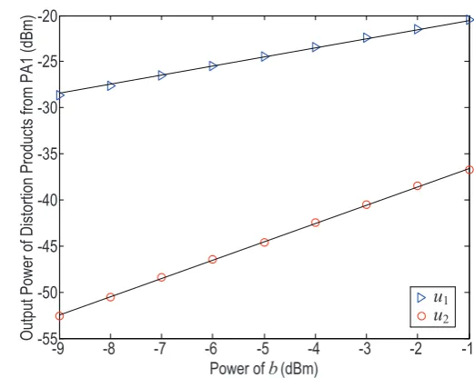
Fig. 2.12 shows how the magnitude of the distortion products u1 and u2 vary
with the strength of the reverse interfering signal b. The signal a from PA1 is maintained constant at the power amplifier’s output saturation level. We notice that
for every 1dB increase in the magnitude of b, u2 increases by 2dB and u1 increases
by 1dB. Thus confirming that the magnitude of u2 is proportional to |a||b|2, and
Power of b(dBm) O ut pu t P ow er o f D is to rt io n P ro du ct s fr om P A 1 (d B m ) u1 u2 -55 -50 -45 -40 -35 -30 -25 -20
-9 -8 -7 -6 -5 -4 -3 -2 -1
Fig. 2.12: Characterization of the reverse IM distortions.
distortion model [6].
Hence, the problem at hand is serious and the general idea of backing off by 1dB
to get a 3dB reduction in distortion does not hold because increasing the isolation
will only control one of the signals (b) contributing to the distortion. What is worse still is that the least responsive distortion product, u1, is also the largest. The
isolation can be increased by either using an isolator to reduce b, or by further antenna separation between PA1 and PA2. The former introduces additional cost
and insertion loss, while the latter requires more real-estate area.
2.5.2
Desensitization/Blocking
Fig. 2.13 illustrates how a strong interfering transmit signal from a colocated
trans-mitter could desensitize/block a receiver. The experiment connects an LNA (of
about 19dB gain) to two signal sources using a power combiner, one generating the
desired signal and the second generating the jammer. The output of the LNA is
connected to a spectrum analyzer. Initially, the figure shows the LNA output with
the desired signal at−51dBm in the presence of a small jamming signal measured at
Unit dBm Ref Lvl
19.6 dBm Ref Lvl
19.6 dBm
RF Att 40 dB RBW 10 kHz
VBW 10 kHz SWT 32 ms
1AVG
Large Jammer Small Jammer
Desired Signal
Jammer
-70 -60 -50 -40 -30 -20 -10 0 10
-80.4 19.6
Span 1.25 MHz 125 kHz/
Center 920.501925 MHz 17dB
Fig. 2.13: Desensitization/Blocking. Spectrum at the LNA output. Desired signal at 920MHz and Jamming signal at 921MHz.
overwhelmed the LNA, and desensitized its gain by 17dB.
2.6
Summary
• The chapter discusses the basic concepts of noise and distortion within wireless radio systems. It defines performance metrics (e.g., noise factor, IP3, etc.) that
characterize the noise and distortion properties of wireless radio systems.
• The basics of an attenuator and a directional coupler are discussed in sections 2.2 and 2.3 respectively.
• Controlled laboratory measurements are used to demonstrate reverse IM3 gen-eration and receiver desensitization at colocated base station settings.
This chapter builds the basics required for the rest of the thesis. The next chapter
investigates previously published literature and proposes potential solutions for the
Chapter 3
Literature Review
Nonlinearity in RF front-ends is an ongoing challenge in the field of wireless
com-munication. While there are many solutions that mitigate distortions and jamming
signals within the receiver front-end, there is little work addressing the issues in a
colocated base station receiver in its entirety. In this chapter, we discuss relevant
solutions for overcoming colocation nonlinearity issues. We examine other research
studies to find potential distortion mitigation techniques for the colocated receivers.
Finally, we summarize our study and outline the basics of two potential solutions,
one for distortions produced within the receiver front-end and the other for reverse
IM distortions generated at a colocated transmitter.
One of the issues of colocation is that the early occupier of the site initially
experiences no such interference problems. Distortions get generated as more
trans-mitters are added to the site. Thus, the initial occupiers of the site would be very
reluctant to adopt a new solution into their transmitters and disrupt operationally
stable systems. Especially, when it incurs further capital expenditures and the
victim service provider is possibly a competitor. Hence, it is less likely that the
colocated victim receiver would get any collaboration from the aggressor jammers.
Therefore, solutions are required that can be independently deployed by the victim
receiver. Further, the victim receiver would prefer solutions that can mitigate the
problem without requiring much modification to its existing hardware and incur
Section 3.1 discusses different filtering solutions that are available for the
coloca-tion problem. Seccoloca-tion 3.2 studies various adaptive cancellacoloca-tion schemes that could
be used to mitigate forward IM products. Section 3.3 proposes an adaptive
can-cellation technique that mitigates forward IM products by canceling the strong
jamming signals before they hit the receiver front-end circuits. Section 3.4
dis-cusses transmitter-end solutions that have been proposed for reverse IM products,
and reviews potential receiver linearization techniques that can be adapted to
de-velop a receiver-end solution. Finally, section 3.5 proposes a receiver postdistortion
cancellation technique for mitigating reverse IM products.
3.1
Filtering Solutions
This family of solutions use passive filters to reject the jamming signals before they
enter the nonlinearities.
3.1.1
Knowledge-based Filtering
The authors of [3] have used computer simulations to model the colocation scenario
and predict the characteristics of the jamming signals. This requires knowledge of
the colocated transceiver specifications and antenna configurations. A fixed
cus-tomized filter is then deployed to mitigate the interference. This makes the solution
unsuitable for dynamic environments. Unfortunately, many cosite scenarios require
a certain level of adaption to handle changing carrier frequencies and ON/OFF
keying of transmitters.
Another approach described in [4] located the jamming signal by scanning the
spectrum with a Fast Fourier Transform (FFT) and then removed it with a
tun-able notch filter. This adds extra filter complexity issues. Secondly, removing the
jammers using such filtering techniques does not help in mitigating the reverse IM
3.1.2
Passive Filtering
RXc TXa
TXb
UEa UEc
UEb Power
Amplifier
Power Amplifier
Post Filtering
Post Filtering
Pre-Filtering
Fig. 3.1: Passive pre and post filtering to mitigate colocated interference issues [17].
Netcom proposes a brute-force solution in [17] for a military frequency hopping
communication system. As seen in Fig. 3.1, it involves the placement of frequency
agile band pass filters in front of receiver LNAs and after the transmitter PAs. The
receiver pre-filtering stops large jamming signals and admits only the desired signal
into the LNA. Likewise, transmitter post-filtering rejects any reverse signal from
en-tering the PAs and stops IM products produced from being transmitted. However,
expensive high-Q cavity filters with low insertion loss would be required to suffi-ciently attenuate the large transmitter signals, which, in some cases, have output
powers of +47dBm (50W) [18]. In addition, frequency agility adds another
dimen-sion of complexity and cost. Overall, it is a commercially unfeasible proposition for
wireless service providers.
3.2
Adaptive Cancellation for Forward IM
Colocation of multiple radio technologies is also a problem within user equipment
(MAC) layer solutions and the physical layer solutions [19]. The most effective MAC
layer solution is to use time slotting/sharing [20] [21]. However, such techniques
reduce the overall throughput of the participating radio technologies. In contrast,
physical layer solutions allow simultaneous operation of the transceivers. The ideal
solution is to remove the coupled aggressor signal before it hits the victim receiver
LNA/mixer circuits. Such a goal could be achieved using adaptive cancellation
techniques.
3.2.1
Single Loop Narrowband Cancellation
MOBILE COMMUNICATION SYSTEM SUB-UNIT
POSITIONING SYSTEM RECEIVER
SUB-UNIT
+
INTERFERENCE SUPPRESSION UNIT BRANCH
OFF UNIT
SUPER-POSITION UNIT INTERFERENCE PATH
COMPENSATION PATH
Fig. 3.2: Transmitter leakage cancellation for a colocated GPS receiver [22].
The proponents of [22] and [23] propose a single-loop adaptive cancellation
sys-tem for colocating a global positioning syssys-tem (GPS) receiver unit within a mobile
communication UE. As seen in Fig. 3.2, the cancellation system couples out a
sam-ple of the interfering mobile communication transmit signal. The compensation path
signal is then adaptively gain-phase adjusted such that it is equal in magnitude and
180◦ out of phase to the interference path signal when coupled back in the receive
path of the GPS unit. This mitigates the interfering mobile communication transmit
can only cancel narrow-band signals. Wideband signal cancellation would require
an accurate delay match of the compensation path to the interference path.
3.2.2
Single Loop Wideband Cancellation
Tx
Rx
Tx Leakage
Phase Aligner
Variable Gain Amplifier
Bandpass Emulation
Filter
Fig. 3.3: Interference cancellation unit for colocated radios [24].
Fig. 3.3 shows how the authors of [24] add an emulation filter in their cancellation
loop to estimate the transfer function of the interference path. This ensures proper
delay matching and allows 15-30dB cancellation of a wideband bluetooth aggressor
signal at the WLAN receiver, both colocated within the same UE.
3.2.3
Multiple-loop Multi-band Cancellation
UE devices operating in frequency division duplex (FDD) also have the problem of
the transmitter acting as an aggressor on to the receiver. The regular solution is to
use passive SAW (surface acoustic wave) duplexing bandpass filters. The transmit
chain bandpass filter stops the radiation of transmitter noise into the receiver’s
desired channel. The receiver path bandpass filter stops the transmitter signal from
sufficient power handling capability when used in base station environments and are
not frequency agile. An alternative approach taken by the authors of [25] propose
an adaptive duplexing circuit for multi-band operation. As seen in Fig. 3.4, the
adaptive duplexer uses a circulator to direct the transmit signal into the antenna
port and to direct the desired signal into the receive path. However, the limited
reverse isolation of the circulator allows leakage of the transmit signal and noise
into the receive path. The authors use a direct feed from the transmitter in an
adaptive double-loop cancellation path to create two nulls, as seen in Fig. 3.4(b),
effectively removing the interfering transmit signal and transmitter noise from the
receiver. Further, delay lines are used to ensure the required matching between the
interference path and the cancellation path such that a 5MHz (WCDMA) wideband
cancellation is achieved at the nulls. The loops achieved about 46dB cancellation of
the transmit signal and 17dB reduction of the transmitter noise at the receiver.
Tx
Rx
h
1h
2+
a
b
c RF
Directional
Coupler CombinerRF
Circulator
Tx Leakage Tx
Signal SignalRx
(a) Adaptive duplexer architecture.
Tx leakage signal
Rx signal
Rx noise Tx noise
Two nulls
f
P
ow
er frequency responseAdaptive duplexer
fRx fTx
(b) Adaptive duplexer provides two nulls at the transmitted frequency and the desired receive fre-quency.
However, in a colocated base station scenario each of the transceivers are
inde-pendent and a direct feed from colocated aggressor transmitters is not likely.
Fur-ther, both papers [24] and [25] publish good cancellation performance, but neither
of them consider noise and distortion generated in the canceling loops themselves.
This is a key factor in any practical deployment, particularly when power levels are
high.
3.3
The Proposed Solution for Forward IM
ADAPTIVE FILTER
FILTER OUTPUT SIGNAL
SOURCE
NOISE SOURCE
PRIMARY INPUT
REFERENCE INPUT
ADAPTIVE NOISE CANCELLER ERROR
0 0
s
!
n
1 1
s
!
n
SYSTEM OUTPUT
z
Fig. 3.5: The adaptive noise canceling concept [26].
The basis of the above mentioned techniques originates from the concept of
adap-tive noise canceling described in [26] and [27]. The method uses a ‘primary’ input
transducer to receive the noise corrupted desired signal and a ‘reference’ transducer
to acquire noise that is correlated in some way to the primary input’s noise. As
shown in Fig. 3.5, the reference input is adaptively filtered and subtracted from the
primary input to obtain the actual desired signal. However, a sample of the desired
signal may also radiate into the reference input and result in self-cancellation. This
can be overcome by placing the transducer close to the interfering noise source and
achieving a sufficiently large interference-to-signal ratio in the reference input. The
original application was for acoustic noise canceling, in which case, the transducers
were microphones. In our work we use antennas to cancel RF jamming signals.


![Fig. 3.1: Passive pre and post filtering to mitigate colocated interference issues [17].](https://thumb-us.123doks.com/thumbv2/123dok_us/7944094.1318650/49.595.153.443.132.367/fig-passive-post-ltering-mitigate-colocated-interference-issues.webp)
![Fig. 3.2: Transmitter leakage cancellation for a colocated GPS receiver [22].](https://thumb-us.123doks.com/thumbv2/123dok_us/7944094.1318650/50.595.191.404.322.537/fig-transmitter-leakage-cancellation-colocated-gps-receiver.webp)
![Fig. 3.3: Interference cancellation unit for colocated radios [24].](https://thumb-us.123doks.com/thumbv2/123dok_us/7944094.1318650/51.595.209.385.205.441/fig-interference-cancellation-unit-colocated-radios.webp)
