Reducing Depth in Constrained PRFs: From Bit-Fixing
to NC
1
∗
Nishanth Chandran
†Srinivasan Raghuraman
‡Dhinakaran Vinayagamurthy
§Abstract
The candidate construction of multilinear maps by Garg, Gentry, and Halevi (Eurocrypt 2013) has lead to an explosion of new cryptographic constructions ranging from attribute-based encryption (ABE) for arbitrary polynomial size circuits, to program obfuscation, and to constrained pseudorandom functions (PRFs). Many of these constructions requireκ-linear maps for largeκ. In this work, we focus on the reduction ofκin certain constructions of access control primitives that are based onκ-linear maps; in particular, we consider the case of constrained PRFs and ABE. We construct the following objects:
• A constrained PRF for arbitrary circuit predicates based on (n+`OR−1)−linear maps (wheren is the input length and`OR denotes the OR-depth of the circuit).
• For circuits with a specific structure, we also show how to construct such PRFs based on (n+`AND− 1)−linear maps (where`AND denotes the AND-depth of the circuit).
We then give a black-box construction of a constrained PRF for NC1 predicates, from any bit-fixing constrained PRF that fixes onlyoneof the input bits to 1; we only require that the bit-fixing PRF have certain key homomorphic properties. This construction is of independent interest as it sheds light on the hardness of constructing constrained PRFs even for “simple” predicates such as bit-fixing predicates.
Instantiating this construction with the bit-fixing constrained PRF from Boneh and Waters (Asiacrypt 2013) gives us a constrained PRF forNC1 predicates that is based only onn-linear maps, with no dependence on the predicate. In contrast, the previous constructions of constrained PRFs (Boneh and Waters, Asiacrypt 2013) required (n+`+ 1)−linear maps for circuit predicates (where `is the totaldepth of the circuit) and
n-linear maps even for bit-fixing predicates.
We also show how to extend our techniques to obtain a similar improvement in the case of ABE and construct ABE for arbitrary circuits based on (`OR+ 1)−linear (respectively (`AND+ 1)−linear) maps.
1
Introduction
The breakthrough work on multilinear maps [GGH13a] has found tremendous applications in various areas of cryptography. It has lead to attribute-based encryption (ABE) for all polynomial size circuits [GGH+13c],
indis-tinguishability obfuscation and functional encryption for general circuits [GGH+13b], constrained pseudorandom
functions [BW13], and so on. Many of these constructions requireκ-linear maps for largeκ. Largerκleads to more inefficient schemes and stronger hardness assumptions. In this work, we are interested in exploring the reduction ofκin such constructions – specifically, we consider the case of constrained PRFs and ABE.
Constrained Pseudorandom Functions. A pseudorandom function (PRF) is a keyed function,Fk(x), that is computationally indistinguishable from a truly random function, even to an adversary who has oracle access to the function (but has no knowledge about the key k). Constrained PRFs (introduced in [BW13, BGI14, KPTZ13]), allow the owner ofkto give out a constrained keykf, for a predicatef, such that any user who haskf can evaluate
∗Research done while all authors were at Microsoft Research, India †Microsoft Research, India; Email:
‡CSAIL, Massachusetts Institute of Technology; Email:
Fk(x) ifff(x) = 1. The security requirement on all pointsx, such thatf(x) = 0 is the same as that of standard PRFs.
Boneh and Waters [BW13] show how to construct constrained PRFs for bit-fixing predicates using ann−linear map (where nis the input length to the PRF), and also how to construct constrained PRFs for arbitrary circuit predicates using an (n+`+ 1)−linear map (where ` is the total depth of the circuit predicate). Constrained PRFs can be used to construct broadcast encryption with small ciphertext length, identity-based key exchange, and policy-based key distribution.
Attribute Based Encryption. Attribute based encryption (ABE) [SW05] allows a more fine-grained access policy to be embedded into public-key encryption. In more detail, in ABE schemes, there is a master authority who ownsskand publishes public parameters as well as a relationR(x, y). A user who encrypts a messagem, creates a ciphertext under some stringx(that can specify some policy), to obtainEncpk(m, x). The master authority can give a user a secret key sky. Now, this user can use sky to decrypt Encpk(m, x) and obtain m iffR(x, y) = 1; otherwise, the user obtains no information aboutm. ABE, for the class of relations R∈NC1 can be constructed based on bilinear maps [GPSW06]. Recently, the work of [GGH+13c] shows how to construct ABE for arbitrary
circuits based on (`+ 1)−linear maps (where`is the depth of the relationRwhen expressed as a boolean circuit), while [GVW13] also show how to construct ABE for arbitrary circuits based on the Learning with Errors (LWE) hardness problem.
1.1
Our Results
In this work, we show the following results:
• We construct constrained PRFs for arbitrary circuit predicates using an (n+`OR−1)−linear map, where
nis the input length to the PRF and `OR denotes the OR-depth of the constraint f when expressed as a
boolean circuit (informally, the OR-depth of a circuit is defined to be the maximum number of OR gates from input wires to the output wire along any path in the circuit). We believe that the reduction in linearity is important even in cases when it is not an asymptotic improvement as lower linearity results in a weaker hardness assumption.
• Next, we construct constrained PRFs for circuit predicates using an (n+`AND−1)−linear map, where
`AND denotes the AND-depth of the constraintf (informally, the AND-depth of a circuit is defined to be
the maximum number of AND gates from input wires to the output wire along any path in the circuit). Although in this construction, we require the circuit to be of a specific structure, we show that for several circuits, our construction reduces the number of levels of multilinear map needed.
• Then, we show (in a black-box manner) how to convert any bit-fixing constrained PRF that fixes onlyone bit1 to 1 into a constrained PRF for NC1 circuits; we only require that the bit-fixing PRF have certain
additive key-homomorphic properties. We believe this construction to be of independent interest as the only known (non-trivial) constructions of constrained PRFs are based on multilinear maps.
By instantiating this construction with the bit-fixing constrained PRF of Boneh and Waters [BW13], we obtain a constrained PRF for all predicatesf ∈NC1 using ann−linear map. In particular, the number of levels in our construction has no dependence onf.
• Finally, we show how to extend our techniques to construct ABE schemes from lesser levels of multi-linear maps.
Similar to [BW13], all our constructions are based on theκ-Multilinear Decisional Diffie-Hellman (κ-MDDH) assumption and achieve selective security (i.e., the adversary must commit to the challenge query at the beginning of the security game); as in [BW13], we can achieve standard security via complexity leveraging. We remark that our techniques can be extended to the constructions of verifiable constrained PRFs [Fuc14, CRV14], thereby leading to a similar lowering of κ.
Other related works. The work of [FKPR14] considers the prefix-fixing constrained PRF from the classical GGM construction [GGM86], and shows how to avoid an exponential (in n) loss in security when going from selective security to adaptive security. Their work also shows that any “simple”’ reduction, that proves full security of the bit-fixing constrained PRF of [BW13], from a non-interactive hardness assumption, must incur an exponential security loss. The work of [HKKW14] shows how to construct adaptively secure constrained PRFs for circuits from indistinguishability obfuscation in the random oracle model. More recently, key-homomorphic constrained PRFs were constructed in [BV15, BFP+15]. Similar to us, Banerjeeet al. [BFP+15] also observe that
[BW13] is “key-homomorphic”.
Security of multilinear maps. After the initial work of Garg et al. [GGH13a], Coron, Lepoint and Tibouchi proposed a multilinear maps construction over the integers [CLT13] also based on ideal lattices. But, Cheon, Han, Lee, Ryu and Stehl´e [CHL+15] proposed an attack which completely broke the CLT scheme by recovering the secret
parameters of the scheme in polynomial time. Coron et al. [CLT15] proposed another candidate construction. This was broken recently by Cheon et al. [CLR15] and Minaud et al. [MF15]. Hu and Jia [HJ15] also recently showed that theκ-MDDH assumption in [GGH13a] does not hold when encodings of zero are provided. Independent of these, Gentry, Gorbunov and Halevi [GGH15] proposed a multilinear maps construction based onrandom lattices but with the map defined with respect to a directed acyclic graph.
We do not rely on the security of any specific multilinear maps scheme. Since we do not give low-level encodings of zero in our construction, any scheme [GGH13a, CLT13, CLT15] which is secure under theκ-MDDH assumption can be used to instantiate our constructions.
1.2
Our Techniques
Our starting point is the constrained PRF construction of [BW13] for arbitrary circuit predicates. We first view this construction differently as follows. Let the PRF in [BW13] be denoted byPRFn+`(u, x), whereuis the key
of the PRF, x, an n-bit string, is the input to the PRF, and PRFn+` denotes that the PRF output is at the (n+`)−level of the multilinear map (where`denotes the depth of the constraintf). Now, in order to give out a constrained key for f, we first pick a random valuerw for every wirew in the circuit. Letj denote the depth of this wire in the circuit. Now, for a given xsuch that f(x) = 1, the idea is to give a key that will enable the user to computePRFn+j(rw, x) for all wireswin the circuit that evaluate to 1 on x. Doing this inductively will allow the compution ofPRFn+`(u, x). Letwbe an output to some gate in the circuit and let A(w), B(w) be the input
wires corresponding to this gate. If this gate is an AND (respectively OR) gate, we give a key, that will allow a user to computePRFn+j(rw, x) from the valuesPRFn+j−1(rA(w), x) AND (respectively OR)PRFn+j−1(rB(w), x).
Free AND construction. Our first observation is that for AND gates, one must be able to compute the PRF value corresponding to w wire iff one has the PRF values corresponding to both A(w) and B(w). Now, suppose the PRF under consideration is “additively homomorphic” in some sense. Then, we observe that given
PRFn+j−1(rA(w), x) andPRFn+j−1(rB(w), x), one can compute PRFn+j−1(rw, x), without the need for additional keys and without jumping a level in the multilinear map as long as we setrA(w)andrB(w) to be random additive
shares ofrw. Now, this ensures that AND gates are “free” in the circuit. The OR gates are handled exactly as in the case of [BW13]. This leads to a construction that only makes use of a (n+`OR−1)−linear map.
While this is the main change made to the construction, the proof of security now requires attention. At a very high level, [BW13] could embed a part of the “hard problem” from the hardness assumption at every layer of the circuit as they give out keys for all gates in the circuits. In our case, we do not have that luxury. In particular, since we do not give any keys for AND gates, the structure of the hard problem may be distorted after multiple evaluations of AND gates. In order to overcome this, we must carefully give out the keys at OR levels to “reset” the problem to be of our preferred form. This enables us to then prove security.
Free OR construction. Now, suppose we turn our attention towards the OR gates alone. Note, that one must be able to compute the PRF value corresponding to wire w iff one has the PRF values corresponding to either
A(w) or B(w). Now, suppose we set rw =rA(w)=rB(w), then this enables the computation ofPRFn+j−1(rw, x) from eitherPRFn+j−1(rA(w), x) orPRFn+j−1(rB(w), x), without the need for additional keys and without jumping
a level in the multilinear map. However, doing this na¨ıvely would lead to a similar “backtracking attack” as the attack described by [GGH+13c] in the context of ABE. In more detail, note that ifA(w) = 0 andB(w) = 1, one
can indeed (rightly) computePRFn+j−1(rw, x) fromPRFn+j−1(rB(w), x) as bothB(w) andware 1. However, this
this would lead to an attack on the security of the PRF. Here, we show that if the circuit had a specific structure, then such a construction can still be made to work. We show that several circuits can be converted to this form (with a polynomial blowup) that results in a reduction in the number of multilinear levels needed. We remark that for the construction (and proof) to succeed, one must carefully select the random key values on the circuit for the constrained key , starting backwards, from the output wire in the circuit.
NC1 construction. While we obtain our construction of constrained PRF forNC1 circuits by combining the above two techniques, we note that the proof of security is tricky and requires the simulator to carefully set the random keys in the simulation. In particular, let x∗ be the challenge input to the PRF. Now, suppose, the simulator must give out a constrained key for a circuitf such thatf(x∗) = 0. The simulator must choose all the random keys of the PRFs on each wire in such a way that for all wires that evaluate to 1 onx∗, the key is either chosen randomly by the simulator or can be computed from values that are chosen randomly by the simulator. We show that this can be indeed done by the simulator, thus resulting in the proof of security.
We then show how to generalize this construction to obtain a constrained PRF for NC1 circuits from any constrained PRF for bit-fixing predicates that fixes only one bit and has certain additively homomorphic properties. We believe this construction to be of independent interest as till date, constrained PRFs for any non-trivial predicate, are known only based on multilinear maps.
Finally, we show how to extend our Free AND/OR techniques to the case of ABE. This gives an ABE based on (`OR + 1)−linear and (`AND+ 1)−linear maps respectively, improving upon the (`+ 1)−linear map
construction of [GGH+13c].
1.3
Organization
In Section 2, we define constrained PRFs and ABE as well as state the hardness assumption that we make. We also present circuit notation that is used in the rest of the paper. In Section 3, we describe our (n+`OR−1)−linear
map construction of constrained PRF for arbitrary circuits. We outline our (n+`AND−1)−linear map construction
in Section 4. We present our n−linear map construction of constrained PRF for NC1 circuits in Section 5 and the black-box construction of constrained PRF for NC1 circuits from bit-fixing constrained PRFs in Section 6. We finally show the extension of our results to ABE in Appendix??.
2
Preliminaries
2.1
Definitions
Constrained Pseudorandom Functions. A pseudorandom function (PRF)F :K × X → Y, is a deterministic polynomial (in security parameter λ) time algorithm, that on input a key k ∈ K and an input x∈ X, outputs
F(k, x)∈ Y. F has a setup algorithmSetup(1λ) that on inputλ, outputs a keyk∈ K.
Definition 2.1. A PRFF :K × X → Y is said to be constrained with respect to a set systemS ⊆ X if there is an additional key space Kc, and there exist algorithms (F.Constrain, F.Evaluate) such that
• F.Constrain(k, S) is a randomized polynomial time algorithm that takes as input a PRF keyk∈ Kand the description of a setS∈ S. It outputs a constrained keykS ∈ Kc which enables the evaluation ofF(k, x) for allx∈S and no otherx;
• F.Evaluate(kS, x) is a deterministic polynomial time algorithm that takes as input a constrained keykS ∈ Kc and an inputx∈ X. IfkS is the output of F.Constrain(k, S) for somek∈ K, then F.Evaluate(kS, x) outputs
F(k, x) ifx∈S and⊥otherwise, where⊥6∈ Y. We will use the shorthandF(kS, x) for F.Evaluate(kS, x).
The security of constrained PRFs informally states that given several constrained keys, as well as the output of the PRF on several points of the adversary’s choice, the PRF looks random at all points that the adversary could not have computed himself. Let F : K × X → Y be a constrained PRF with respect to a set systemS. Define two experimentsExp0 andExp1. Forb∈ {0,1},Expb proceeds as follows:
2. The adversary is given access to the following oracles:
• F.Constrain: Given a setS∈ S, ifS∩C=∅, the oracle returns F.Constrain(k, S) and updatesV ←V∪S; otherwise, it returns⊥.
• F.Evaluate: Given an input x ∈ X, if x 6∈ C, the oracle returns F(k, x) and updates V ← V ∪x; otherwise, it returns⊥.
• Challenge: Givenx∈ X wherex6∈V, ifb= 0, the oracle returns F(k, x); ifb= 1, the oracle returns a random (consistent)y∈ Y. Cis updated asC←C∪x.
3. The adversary finally outputs a bitb0 ∈ {0,1}.
4. Forb ∈ {0,1}, define Wb to be the event that thatb0 = 1 in experimentExpb. The adversary’s advantage
AdvA,F,S(λ) is defined to be|Pr[W0]−Pr[W1]|.
Definition 2.2. A constrained PRF F :K × X → Y, is said to be secure, if for all PPT adversaries A, we have that AdvA,F,S(λ), is negligible inλ.
Remark. When constructing constrained pseudorandom functions, it will be more convenient to work with the definition where the adversary is allowed to issue only a single challenge query. A standard hybrid argument shows that this definition is equivalent to the one where an adversary is allowed to issue multiple challenge queries. A constrained PRF is selectively secure if the adversary commits to this single challenge query at the beginning of the experiment.
Attribute-based Encryption. An attribute-based encryption (ABE) scheme has the following algorithms:
• Setup(1λ, n, `): This algorithm takes as input the security parameterλ, the lengthnof input descriptors in the ciphertext, and a bound` on the circuit depth. It outputs the public parametersP P and the master secret keyM SK.
• Encrypt(P P, x, M): This algorithm takes as input the public parameters, x ∈ {0,1}n (representing the assignment of boolean variables) and a messageM. It outputs a ciphertextCT.
• KeyGen(M SK, f): This algorithm takes as input the master secret key and a circuitf. It outputs a secret keySK.
• Decrypt(SK, CT): This algorithm takes as input a secret key and ciphertext and outputs eitherM or⊥.
The correctness of the ABE requires that for all messages M, for all x∈ {0,1}n, for all depth ` circuits f, with f(x) = 1, ifEncrypt(P P, x, M) outputsCT, and KeyGen(M SK, f) outputsSK, whereP P andM SK were obtained as the output ofSetup(1λ, n, `), thenDecrypt(SK, CT) =M. The security of an ABE scheme is defined through the following game between a challengerChalland adversaryAdvas described below:
• Setup. ChallrunsSetup(1λ, n, `) and givesP P to Adv; it keepsSK to itself.
• Phase 1. Advmakes any polynomial number of queries for circuit descriptionsf of its choice. Challreturns
KeyGen(M SK, f).
• Challenge. Advsubmits two equal length messagesM0 andM1 as well as an x∗∈ {0,1}such that for all
f queried in Phase 1,f(x∗) = 0. Challflips a bitband returnsCT∗=Encrypt(P P, x∗, Mb) toAdv.
• Phase 2. Phase 1 is repeated with the restriction thatf(x∗) = 0 for all queriedf.
• Guess. Advoutputs a bitb0.
Definition 2.3. The advantage ofAdvin the above game is defined to be|Pr[b0 =b]−1
2|. An ABE for circuits
2.2
Assumptions
Leveled multilinear groups. We assume the existence of a group generatorG, which takes as input a security paramter 1λ and a positive integer κ to indicate the number of levels. G(1λ, κ) outputs a sequence of groups
~
G= (G1, . . . ,Gκ) each of large prime orderp >2λ. In addition, we let gi be a canonical generator of Gi that is known from the group’s description. We let g=g1. We assume the existence of a set of multilinear maps{ei,j : Gi×Gj →Gi+j|i, j ≥1;i+j ≤κ}. The mapei,j satisfies the following relation: ei,j(gai, gjb) =giab+j,∀a, b∈Zp. When the context is obvious, we will drop the subscriptsi, j. For example, we may simply writee(ga
i, gjb) =gabi+j. We define theκ-Multilinear Decisional Diffie-Hellman (κ-MDDH) assumption [GGH13a] as follows:
Assumption 2.1. (κ-Multilinear Decisional Diffie-Hellman: κ-MDDH) The κ-Multilinear Decisional Diffie-Hellman (κ-MDDH) problem is as follows: A challenger runsG(1λ, κ) to generate groups and generators of order
p. Then it picks randomc1, . . . , cκ+1∈Zp. The assumption states that giveng=g1, gc1, . . . , gcκ+1, it is hard to
distinguish the elementT =g
Q
j∈[κ+1]cj
κ from a random group element inGκwith better than negligible advantage in λ.
2.3
Circuit Notation
We will consider layered circuits, where a gate at2depthjwill receive both of its inputs from wires at depthj−1.
We also assume that all NOT gates are restricted to the input level. Similar to [BW13], we restrict ourselves to monotonic circuits where gates are either AND or OR gates of two inputs.3
Formally, our circuits will be a five tuplef = (n, q, A, B,GateType). We let n be the number of inputs and
q be the number of gates. We defineinputs = [n], Wires = [n+q] and Gates = [n+q]\[n]. The wire n+q is designated as the output wire,outputwire. A:Gates→Wires\{outputwire}is a function whereA(w) identifiesw’s first incoming wire and B :Gates→Wires\{outputwire} is a function where B(w) identifiesw’s second incoming wire. Finally,GateType:Gates→ {AND,OR}is a function that identifies a gate as either an AND gate or an OR gate. We let w > B(w)> A(w). Also, define three functions: tot-depth(w),AND-depth(w), andOR-depth(w) that are all 1, whenw∈inputs, and in general are equal to the number of gates (respectively AND and OR gates) on the shortest path to an input wire plus one. We let f(x) be the evaluation of f on the inputx∈ {0,1}n, and
fw(x) be the value of the wirewon the input x.
3
A Free-AND Circuit-predicate Construction
We show how to construct a constrained PRF for arbitrary polynomial size circuit predicates, without giving any keys for AND gates, based on κ = (n+`OR−1)−linear maps, where `OR denotes the OR-depth of the circuit.
The starting point of our construction is the constrained PRF construction of [BW13] which is based on the ABE for circuits [GGH+13c]. [BW13] works with layered circuits. For ease of exposition, we assume a layered circuit
where all gates in a particular layer are of the same type (either AND or OR). Circuits have a single output OR gate. Also a layer of gates is not followed by another layer of the same type. We stress that these are only for the purposes of exposition and can be removed as outlined later on in the section.
3.1
Construction
F.Setup(1λ, n, `OR):
The setup algorithm takes as input the security parameter λ, the bit length, n, of PRF inputs and `OR, the
maximum OR-depth4 of the circuit. The algorithm runs G(1λ, κ = n+`
OR−1) and outputs a sequence of
groups G~ = (G1, . . . ,Gκ) of prime orderpwith canonical generatorsg1, . . . , gκ, whereg=g1. It chooses random
exponents u∈Zp and (d1,0, d1,1), . . . ,(dn,0, dn,1)∈Z2p and computesDm,β=gdm,β form∈[n] andβ ∈ {0,1}. It then sets the key of the PRF as:
k= (G~, p, g1, . . . , gκ, u, d1,0, d1,1, . . . , dn,0, dn,1, D1,0, D1,1, . . . , Dn,0, Dn,1)
The PRF isF(k, x) =gu
Q
m∈[n]dm,xm
κ , wherexmis themth bit ofx∈ {0,1}n.
2When the term depth is used, it is synonymous to the notion oftot-depthdescribed ahead. 3These restrictions are mostly useful for exposition and do not impact functionality.
F.Constrain(k, f = (n, q, A, B,GateType)):
The constrain algorithm takes as input the key kand a circuit descriptionf. The circuit hasn+qwires withn
input wires, qgates and the wiren+qdesignated as the output wire.
To generate a constrained keykf, the key generation algorithm chooses randomr1, . . . , rn∈Zp, where we think of the random valuerwas being associated with the wirew. For eachw∈[n+q−1]\[n], ifGateType(w) = AND, it sets rw=rA(w)+rB(w) (where + denotes addition in the groupZp); otherwise, it choosesrw∈Zp at random. Finally, it setsrn+q=u.
The first part of the constrained key is given out as simply all Di,β for i ∈ [n] and β ∈ {0,1}. Next, the algorithm generates key components. The structure of the key components depends on whetherwis an input wire or an output of an OR gate. For AND gates, we do not need to give out any keys. The key components in each case are described below.
• Input wire. By convention, if w ∈ [n], then it corresponds to the w-th input. The key component is:
Kw=grwdw,1.
• OR gate. Letj =OR-depth(w). The algorithm chooses random aw, bw∈Zp. Then, the algorithm creates key components:
Kw,1=gaw, Kw,2=gbw, Kw,3=g
rw−aw·rA(w)
j−1 , Kw,4=g
rw−bw·rB(w) j−1
The constrained keykf consists of all these key components along with{Di,β}fori∈[n] andβ∈ {0,1}.
F.Evaluate(kf, x):
The evaluate algorithm takes as input a constrained key kf for the circuit f and an input x ∈ {0,1}n. The algorithm first checks that f(x) = 1, and if not, it aborts. Consider the wire w at OR-depth j. If fw(x) = 1, then, the algorithm computes Ew=g
rwQm∈[n]dm,xm
n+j−1 . If fw(x) = 0, then nothing is computed for that wire. The algorithm proceeds iteratively starting with computing E1and proceeds, in order, to compute En+q. Computing these values in order ensures that the computation on a lower-depth wire that evaluates to 1 will be defined,
before the compution on a higher-depth wire. Sincern+q =u,En+q=g uQ
m∈[n]dm,xm
n+`OR−1 . We show how to compute
Ew for allwwherefw(x) = 1, case-wise, according to whether the wire is an input, an OR gate or an AND gate. Define D=D(x) =g
Q
m∈[n]dm,xm
n , which is computable through pairings.
• Input wire. Supposefw(x) = 1. Through pairing operations, the algorithm computesg
Q
m∈[n]\{w}dm,xm
n−1 . It
then computes:
Ew=e
Kw, g Q
m∈[n]\{w}dm,xm n−1
=grw
Q
m∈[n]dm,xm n
• OR gate. Letj=OR-depth(w). The computation is performed iffw(x) = 1. Note that in this case, at least one offA(w)(x) andfB(w)(x) must be 1. IffA(w)(x) = 1, the algorithm computes:
Ew=e(EA(w), Kw,1)·e(Kw,3, D)
=egrA(w)
Q
m∈[n]dm,xm
n+j−2 , g
aw
·egrw−aw·rA(w)
j−1 , g
Q
m∈[n]dm,xm n
=grw
Q
m∈[n]dm,xm n+j−1
Otherwise, we have fB(w)(x) = 1 and the algorithm computes Ew from EB(w), Kw,2, Kw,4 in a similar
manner.
• AND gate. Let j = OR-depth(w). The computation is performed if fw(x) = 1. Note that in this case,
fA(w)(x) =fB(w)(x) = 1. The algorithm computes:
Ew=EA(w)·EB(w)=g
rA(w)Qm∈[n]dm,xm
n+j−1 ·g
rB(w)Qm∈[n]dm,xm
n+j−1 =g
rwQm∈[n]dm,xm n+j−1
The procedures above are evaluated in order for allw for which fw(x) = 1. Thus, the algorithm computes
En+q =g uQ
m∈[n]dm,xm
3.2
Proof of Pseudorandomness
The correctness of the constrained PRF is verifiable in a straightforward manner. The security proof is in the selective security model (where the adversary commits to the challenge input x∗ at the beginning of the game). To get full security, the proof will use the standard complexity leveraging technique of guessing the challengex∗; this guess will cause a loss of a 1/2n-factor in the reduction.
Theorem 3.1. If there exists a PPT adversary A that breaks the pseudorandomness of our circuit-predicate construction for n-bit inputs with advantage (λ), then there exists a PPT algorithm B that breaks the κ = (n+`OR−1)−Multilinear Decisional Diffie-Hellman assumption with advantage (λ)/2n.
Proof. The algorithmBfirst receives aκ= (n+`OR−1)−MDDH challenge consisting of the group sequence
de-scriptionG~ andg=g1, gc1, . . . , gcκ+1along withT, whereTis eitherg
Q
m∈[κ+1]cm
κ or a random group element inGκ.
Setup:
It chooses anx∗ ∈ {0,1}n uniformly at random. Next, it chooses random z
1, . . . , zn ∈Zp and setsDm,β =gcm whenx∗m=βandgzm otherwise, form∈[n] andβ∈ {0,1}. This corresponds to settingd
m,β=cmwhenx∗m=β andzmotherwise. It then implicitly setsu=cn+1·cn+2·. . .·cn+`OR. The setup is executed as in the construction.
Constrain:
Suppose a query is made for a secret key for a circuit f = (n, q, A, B,GateType). If f(x∗) = 1, then B aborts. Otherwise, B generates key components for every wirew, case-wise, according to whetherw is an input wire or an OR gate as described below.
Input wire. By convention, ifw∈[n], then it corresponds to thew-th input. Ifx∗w= 1, thenBchoosesηw=rw at random. The key component is:
Kw= (Dw,1)rw=grwdw,1
If x∗w = 0, then B implicitly sets rw = cn+1+ηw, where ηw ∈ Zp is a randomly chosen element. The key component is:
Kw= (gcn+1·gηw)zw =grwdw,1
OR gate. Suppose thatw∈Gatesand thatGateType(w) = OR. In addition, letj=OR-depth(w). In order to show that Bcan simulate all the key components, we shall additionally show the following property:
Property 3.1. For any gate w∈Gates,Bwill be able to computegrw
j , wherej=OR-depth(w).
We will prove the above property through induction on the OR-depthj; doing this will enable us to prove that
Bcan compute all the key components required to give out the constrained key . The base case of the input wires (j= 1) follows as we know that for an input wirew,Bcan computegrw, wherer
wis of the formηworcn+1+ηw.
We now proceed to show the computation of the key-components. In each case, we show that property 1 is satisfied.
CASE 1: If fw(x∗) = 1, then B chooses ψw = aw, φw = bw and ηw = rw at random. Then, B creates key components:
Kw,1=gaw, Kw,2=gbw, Kw,3=g
rw−aw·rA(w)
j−1 , Kw,4=g
rw−bw·rB(w) j−1
By virtue of of property 1, sinceOR-depth(A(w)) =OR-depth(B(w)) =j−1, by the induction hypothesis, we know that Bcan computegrA(w)
j−1 and g
rB(w)
j−1 . Hence,Bcan compute the above key-components, as the remaining
exponents were all chosen at random by B. Further, since rw was chosen at random, note that gjrw can be be computed for this wire, and hence property 1 holds for this wire as well (at OR-depthj).
CASE 2: If fw(x∗) = 0, then B implicitly sets rw = cn+1 ·. . . ·cn+j +ηw, where ηw ∈ Zp is a randomly chosen element. Since ηw was chosen at random, note that gjrw can be be computed for this wire (since
gcn+1·...·cn+j
1. Suppose the level before the current level consists of the inputs.Bwould know the values ofηA(w)andηB(w),
since for input wires, these values are always chosen at random. In this case,Bimplicitly setsaw=cn+j+ψw andbw=cn+j+φw, whereψw, φw∈Zp are randomly chosen elements. Then,Bcreates key components:
Kw,1=gcn+j+ψw=gaw, Kw,2=gcn+j+φw=gbw,
Kw,3=g
ηw−cn+j·ηA(w)−ψw(cn+1·...·cn+j−1+ηA(w))
j−1 =g
rw−aw·rA(w)
j−1 ,
Kw,4=g
ηw−cn+j·ηB(w)−φw(cn+1·...·cn+j−1+ηB(w))
j−1 =g
rw−bw·rB(w) j−1
B is able to create the last two key components due to a cancellation. Since fA(w)(x∗) = fB(w)(x∗) = 0,
B would have set rA(w) = cn+1·. . .·cn+j−1+ηA(w) and rB(w) = cn+1 ·. . .·cn+j−1+ηB(w). Further,
gcn+1·...·cn+j−1
j−1 can be computed usingj−1 pairings ofgcm,n+ 1≤m≤n+j−1.
2. Suppose the level before the current level consists of AND gates. SincefA(w)(x∗) = 0, we have two cases:
either one of fA(A(w))(x∗) and fB(A(w))(x∗) is zero, or both of them are zero. B sets aw = cn+j+ψw in the former case, and aw = 12cn+j +ψw in the latter case, where ψw ∈ Zp is a randomly chosen element. Similarly, sincefB(w)(x∗) = 0, we have two cases: either one offA(B(w))(x∗) andfB(B(w))(x∗) must be zero,
or both of them must be zero. Bsetsbw=cn+j+φwin the former case, andbw=12cn+j+φwin the latter case, whereφw∈Zp is a randomly chosen element. Then, Bcreates key components:
Kw,1=gaw, Kw,2=gbw, Kw,3=g
rw−aw·rA(w)
j−1 , Kw,4=g
rw−bw·rB(w) j−1
We now show that these components can indeed be computed in every case. Note that the first two compo-nents can be computed in every case. ConsiderKw,3(a similar argument holds for Kw,4).
(a) Consider the first case, where one of fA(A(w))(x∗) and fB(A(w))(x∗) is zero. In particular, without
loss of generality, assume that fA(A(w))(x∗) = 0 and fB(A(w))(x∗) = 1. Hence, B must have set
rA(A(w))=cn+1·. . .·cn+j−1+ηA(A(w)) andrB(A(w))=ηB(A(w)). SinceA(w) is an AND gate, we would
haverA(w)=rA(A(w))+rB(A(w))=cn+1·. . .·cn+j−1+ηA(A(w))+ηB(A(w)). Hence, we have:
Kw,3=g
ηw−cn+j(ηA(A(w))+ηB(A(w)))−ψw(cn+1·...·cn+j−1+ηA(A(w))+ηB(A(w))) j−1
=grw−aw·rA(w) j−1
which can be computed as follows. We know the values ofηA(A(w))andηB(A(w)). Further,g
cn+1·...·cn+j−1 j−1
can be computed usingj−1 pairings ofgcm,n+ 1≤m≤n+j−1. Hence the key component can be computed.
(b) Consider the second case, wherefA(A(w))(x∗) =fB(A(w))(x∗) = 0. Hence, B must have setrA(A(w)) =
cn+1·. . .·cn+j−1+ηA(A(w)) andrB(A(w)) =cn+1·. . .·cn+j−1+ηB(A(w)). SinceA(w) is an AND gate,
we would haverA(w)=rA(A(w))+rB(A(w))= 2cn+1·. . .·cn+j−1+ηA(A(w))+ηB(A(w)). Hence, we have:
Kw,3=g
ηw−12cn+j(ηA(A(w))+ηB(A(w)))−ψw(2cn+1·...·cn+j−1+ηA(A(w))+ηB(A(w))) j−1
=grw−aw·rA(w) j−1
which can be computed as outlined in the former case.
Thus, the four key components can be given out in every case.
AND gate. We now discuss the case of the AND gate. Suppose thatw∈Gatesand thatGateType(w) = AND. In addition, letj=OR-depth(w). Bimplicitly setsrw=rA(w)+rB(w). Note that we need not choose any awor
bw. In fact,rw is being chosen because the key components being given out for the OR gates involverA(w), etc.,
which may potentially be from AND gates. Clearly, property 1 holds here as well, i.e., grw j =g
rA(w)
j ·g
rB(w)
j can
be be computed for this wire, sincegrA(w)
j andg
rB(w)
j can be computed by virtue of of property 1.
Finally, we set, for the output wirew=n+q,ηw= 0, so thatrw=uinB’s internal view. It is easy to see that
chosen at random and in the game executed byB, they are either chosen at random or are values offset by some random valuesψw and φw, respectively. Forw∈[n+q−1],rw also has the same distribution in the real game and the game executed byB. This is true, since in the real game, they are chosen so that randomness on the input wires of an AND gate add up to the randomness on its output wire, and they are chosen at random for an OR gate, while in the game executed byB, they are chosen in the exact same way, where being “chosen at random” is either truly satisfied or are fixed values are offset by randomηw values. Now, we look atrn+q. In the real game,
it is a fixed value u, and in the game executed by B, by settingηn+q = 0,rn+q =cn+1·cn+2·. . .·cn+`OR =u
internally. Hence, they too have the same distribution. Hence all the parameters in the real game and game executed byBhave the identical distribution.
Evaluate:
Suppose a query is made for a secret key for an input x ∈ {0,1}n. If x = x∗, then B aborts. Otherwise, B identifies an arbitrary t such that xt 6= x∗t. Through `OR pairings of gcm, n+ 1 ≤ m ≤ n+`OR, it computes
H =gu `OR =g
cn+1·...·cn+`OR
`OR . Then, through pairing ofDm,xm∀m∈[n]\{t}, it computesg Q
m∈[n]\{t}dm,xm
n−1 and raises
it to dt,xt =zt to getH
0 =gQm∈[n]dm,xm
n−1 . Finally, it computes H00 =e(H, H0) =g
uQ
m∈[n]dm,xm
n+`OR−1 =F(k, x) and
outputs it. Eventually,Awill issue a challenge input ˜x. If ˜x=x∗,Bwill return the valueT and output the same bit asAdoes as its guess. If ˜x6=x∗,Boutputs a random bit as its guess.
This completes the description of the adversaryB. We first note that in the case whereT is part of a MDDH tuple, the real game and game executed byBhave the identical distribution. Secondly, in both cases (i.e., whether or notT is part of the MDDH tuple), as long asBdoes not abort, once again, the real game and game executed by Bhave the identical distribution, except for the output ofB on the challenge queryx∗. We now analyze the probability thatB’s guess was correct. Letδ0 denoteB’s output and letδdenote whetherT is an MDDH tuple or not,δ, δ0 ∈ {0,1}. Now
Pr[δ0 =δ] = Pr[δ0=δ|abort] Pr[abort] + Pr[δ0=δ|abort] Pr[abort]
=1 2(1−2
−n) + Pr[δ0=δ|abort]·(2−n)
=1 2(1−2
−n) +
1 2 +
·(2−n) = 1 2+·(2
−n)
The set of equations shows that the advantage of B is(λ)/2n. This completes the proof of the theorem, which establishes the pseudorandomness property of the construction. Hence, the constrained PRF construction for the circuit-predicate case is secure under theκ-MDDH assumption.
Removing the restrictions. The restriction thatGateType(n+q) = OR enables us to set randomness as we do in the scheme above. But this restriction can be easily removed by setting the randomness corresponding to the last level of OR gates (or the input wires in case there is no OR gate in the circuit) appropriately so thatrn+q ends up beingu.
The restriction that a layer of gates cannot follow another layer of the same type of gates can also be overcome. The case of several consecutive layers of OR gates poses no threat since we move up one level in the multilinear maps for layers of OR gates and hence the current proof method works as is. The case of several consecutive layers of AND gates can be handled by even more careful choices of the randomness aw and bw. When we had only one layer of AND gate (before a layer of OR gates), for an OR gate at OR-depthj, we set aw to be either
1·cn+j +ψw or 12 ·cn+j +ψw depending on whether rA(w) = 1·cn+1·. . .·cn+j−1+ηA(A(w))+ηB(A(w)) or
rA(w)=2·cn+1·. . .·cn+j−1+ηA(A(w))+ηB(A(w)). Similarly, we setbwin accordance withrB(w). Now, when there
are more than one layers of AND gates consecutively, for an OR gate atOR-depthj just after these AND gates, we setaw(resp. b(w)) to be 1kcn+j+ψwwherekis the coefficient ofcn+1·. . .·cn+j−1inrA(w)(resp. rB(w)). We
present an illustration of this technique in Appendix??.
rL
w
rR,1
w .. . rR,i
w .. .
rwR,∆
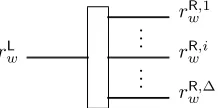
Figure 1: FANOUT-gate
OR-depth of the circuit being d/2 now. So even in the worst case we get improvements in parameters using our scheme.
4
A Free-OR Circuit-predicate Construction
In this section, we show how to construct a constrained random function for polynomial size circuit predicates of a specific form, without giving any keys for the OR gates. Once again, we base our construction on multilinear maps and on theκ-MDDH assumption; howeverκin our construction will only depend onn(the size of the input to the PRF) and now, the AND-depth of the circuit (informally, this is the maximum number of AND gates from input wires to the output wire along any path). Once again, the starting point of our construction is the constrained PRF construction of Boneh and Waters [BW13] which is based on the attribute-based encryption construction for circuits [GGH+13c]. We restrict the class of boolean circuits to be of a specific form. We assume layered circuits
and that all gates in a particular layer are of the same type (either AND or OR). We assume that a layer of gates is not followed by another layer of the same type of gates. We also assume that all AND gates have a fanout of 15.
We introduce here a “gadget” which we call a “FANOUT-gate”. This is done in order to deal with OR gates in the circuit that have a fanout greater than 1. To this end, we assume that a FANOUT-gate is placed just after the OR gate under consideration. We view such OR gates also to have a fanout of 1 and without loss of generality assume that the FANOUT-gate alone has a fanout greater than 1. However, we do not treat the FANOUT-gate while calculating the total depth of the circuit, etc. It is merely a construct which allows us to deal only with OR gates having fanout 1.
4.1
Construction
The setup and the PRF construction is identical to the construction in Section 3. We now outline the constrain and evaluate algorithms.
F.Constrain(k, f = (n, q, A, B,GateType)):
The constrain algorithm takes as input the key kand a circuit descriptionf. The circuit hasn+qwires withn
input wires, qgates and the wiren+q designated as the output wire. Assume that all gates have fanout 1 and that FANOUT-gates have been inserted at places where the gates have a fanout greater than 1.
To generate a constrained keykf, the key generation algorithm setsrn+q =u, where we think of the random value rw as being associated with the wire w. Hence, in notation, if a gate w has fanout greater than 1, then, notation-wise, rwwould have mutliple values: one associated with each of the fanout wires of the FANOUT-gate and one associated with the wire leading out of the gatewitself. We introduce notation for the same below.
Consider a FANOUT-gate placed after wirew, as shown in Figure 1. We denote byrL
w the randomness on the wire going as input to the FANOUT-gate (the actual output wire of the gate under consideration) and byrR,i
w the randomness on the ith fanout wire of the FANOUT-gate (there would be as many of these as the fanout of the gate w), wherei∈[∆] and ∆ is the fanout of the wirew.
We now describe how the randomness for each wire is set. For eachw∈[n+q]\[n], ifGateType(w) = OR, it setsrA(w)=rB(w)=rw, otherwise, it choosesrA(w)andrB(w)at random. The case of FANOUT-gates is handled
as follows. Note that the above description already takes care of setting randomness on all the fanout wires of
5This can always be ensured for circuits that have alternating AND and OR layers. Suppose there is an AND gate with fanout
the FANOUT-gate. The randomness for the input wire to the FANOUT-gate (the output wire of the gate with fanout greater than 1) is chosen at random. Note that this completely describes how randomness on all wires in the circuit are chosen.
The first part of the constrained key is given out as simply all Di,β for i ∈ [n] and β ∈ {0,1}. Next, the algorithm generates key components. The structure of the key components depends on whetherwis an input wire or an output of an AND gate. For OR gates, we do not need to give out any keys, hence the name Free-OR. But, we also need to give out special key components for the FANOUT-gates. The key components in each case are described below.
• Input wire
By convention, ifw∈[n], then it corresponds to thew-th input. The key component is:
Kw=grwdw,1
• AND gate
Suppose thatw∈Gatesand thatGateType(w) = AND. In addition, letj=AND-depth(w). The algorithm chooses randomaw, bw∈Zp. Then, the algorithm creates key components:
Kw,1=gaw, Kw,2=gbw, Kw,3=g
rw−aw·rA(w)−bw·rB(w) j−1
• FANOUT-gate
Suppose thatw ∈Gates, GateType(w) = OR and that the fanout of w is greater than 1. In addition, let
j = AND-depth(w). In this case, a FANOUT-gate would have been placed after w. Let rL
w denote the randomness on the wire going as input to the FANOUT-gate (the actual output wire of the gate under consideration) and letrR,i
w denote the randomness on theith fanout wire of the FANOUT-gate (there would be as many of these as the fanout of the gatew). The keys given out are:
Kw,w0,i=g(
rR,i w−rwL) j−1
for alli∈[∆], where ∆ is the fanout of the gatew.
The constrained keykf consists of all these key components along with{Di,β}fori∈[n] andβ∈ {0,1}.
F.Evaluate(kf, x):
The evaluate algorithm takes as input a constrained keykf for the circuitf = (n, q, A, B,GateType) and an input
x∈ {0,1}n. The algorithm first checks thatf(x) = 1, and if not, it aborts.
Consider the wire w at AND-depth j. If fw(x) = 1, then, the algorithm computes Ew = g
rwQm∈[n]dm,xm
n+j−1 .
If fw(x) = 0, then nothing needs to be computed for that wire. The algorithm proceeds iteratively starting with computing E1 and proceeds, in order, to computeEn+q. Computing these values in order ensures that the computation on a lower-depth wire that evaluates to 1 will be defined before the computation for a higher-depth
wire. Since rn+q =u,En+q=g uQ
m∈[n]dm,xm n+`AND−1 .
We show how to computeEwfor allwwherefw(x) = 1, case-wise, according to whether the wire is an input, an OR gate, an AND gate or a fanout wire of a FANOUT-gate. Define D = D(x) = g
Q
m∈[n]dm,xm
n , which is
computable throughnpairing operations.
• Input wire
By convention, if w ∈ [n], then it corresponds to the w-th input. Supposefw(x) = 1. Through pairing operations, the algorithm computesg
Q
m∈[n]\{w}dm,xm
n−1 . It then computes:
Ew=e
Kw, g Q
m∈[n]\{w}dm,xm n−1
=grw
Q
m∈[n]dm,xm n
• OR gate
Consider a wirew∈GateswithGateType(w) = OR. The computation is performed iffw(x) = 1. Note that in this case, at least one offA(w)(x) andfB(w)(x) must be 1. Hence, we must have been able to evaluate at
least one ofEA(w) andEB(w). Since, for an OR gate,rA(w)=rB(w) =rw, we haveEw=EA(w)=EB(w),
• AND gate
Consider a wirew∈GateswithGateType(w) = AND. In addition, letj =AND-depth(w). The computation is performed iffw(x) = 1. Note that in this case, bothfA(w)(x) andfB(w)(x) must be 1. The algorithm
computes:
Ew=e(EA(w), Kw,1)·e(EB(w), Kw,2)·e(Kw,3, D)
=egrA(w)
Q
m∈[n]dm,xm
n+j−2 , g
aw
·egrB(w)
Q
m∈[n]dm,xm
n+j−2 , g
bw
·
egrA(w)−aw·rA(w)−bw·rB(w)
j−1 , g
uQ
m∈[n]dm,xm n
=grw
Q
m∈[n]dm,xm n+j−1
• FANOUT-gate
LetrwL denote the randomness on the wire going as input to the FANOUT-gate (the actual output wire of the gate under consideration) and letrwR,i denote the randomness on theith fanout wire of the FANOUT-gate (there would be as many of these as the fanout of the gatew). The computation is performed iffw(x) = 1. In coherence with the previous notation, we define the quantitiesEwL and EwR,i. Note that the EwL would have been computed. It then computes:
EwR,i=e(Kw,w0,i, D)·EwL =g
rRw,iQ
m∈[n]dm,xm n+j−1
The procedures above are evaluated in order for allw for which fw(x) = 1. Thus, the algorithm computes
En+q =g uQ
m∈[n]dm,xm
n+`−1 =F(k, x).
5
Combining the Free-AND and Free-OR Techniques
In this section, we show that for the case ofNC1, we can indeed combine the Free-AND and Free-OR techniques to obtain a construction that has Free-ANDs and Free-ORs. While the main reason that the technique works is that forNC1circuits we can consider only boolean formulas, proving that our construction is secure is non-trivial (and different from the case of ABE).
5.1
An NC
1-predicate Construction
We construct a constrained PRF for arbitrary NC1 circuit predicates, without giving any keys for AND as well as OR gates. Again, we base our construction on the κ-MDDH assumption; howeverκ in our construction will only depend onn(the size of the input to the PRF) andnoton the circuit in any way. We will be dealing with circuits of the form described in Section 2.3.
5.2
Construction
F.Setup(1λ,1n):
The setup algorithm that defines the master secret key and the PRF is identical to the setup algorithm from Section 3 withκ=ninstead ofn+`OR−1.
F.Constrain(k, f = (n, q, A, B,GateType)):
The algorithm sets rn+q = u. For each w ∈ [n+q]\[n], if GateType(w) = OR, it sets rA(w) = rB(w) = rw, otherwise, it choosesrA(w)at random and setsrB(w)=rw−rA(w). Since the fanout of all gates is 1, for any wire
w ∈ [n+q]\[n], rw would have been uniquely set. However, since the same inputs may be re-used in multiple gates, for any wire w∈[n],rw may have multiple values (as many as the fanout of the input wire), i.e., different randomness values for each use of the input wire (to different gates). Note that this procedure sets randomness on all wires in the circuit. The first part of the constrained key (kf) is given out as simply allDi,β fori∈[n] and
β ∈ {0,1}. The remaining key components are: Kw,i =grw,idw,1,∀i ∈ [∆], where ∆ is the fanout of the input wire w.
The evaluate algorithm takes as input a constrained key kf and an input x ∈ {0,1}n. The algorithm first checks that f(x) = 1, and if not, it aborts. Consider the wire w. Iffw(x) = 1, then, we show how to compute6
Ew=g
rwQm∈[n]dm,xm
n , case-wise, according to whether the wire is an input, an OR gate or an AND gate.
• Input wire. Through pairing operations, compute g
Q
m∈[n]\{w}dm,xm
n−1 . Then compute: Ew,i =
eKw,i, g Q
m∈[n]\{w}dm,xm n−1
=grw,i
Q
m∈[n]dm,xm
n ∀i∈[∆], where ∆ is the fanout of the input wirew.
• OR gate. In this case, at least one offA(w)(x) and fB(w)(x) must be 1. Hence, we can evaluate at least
one of EA(w) and EB(w). Since, for an OR gate, rA(w) =rB(w) = rw, Ew = EA(w) =EB(w), can now be
computed.
• AND gate. In this case,fA(w)(x) =fB(w)(x) = 1. The algorithm computes:
Ew=EA(w)·EB(w)=g
rA(w)Q
m∈[n]dm,xm
n ·g
rB(w)Q
m∈[n]dm,xm
n =g
rwQm∈[n]dm,xm n
The procedures above are evaluated, in order, for allw for which fw(x) = 1. Thus, the algorithm computes
En+q =g uQ
m∈[n]dm,xm
n =F(k, x).
5.3
Proof of Pseudorandomness
The correctness of the constrained PRF is verifiable in a straightforward manner. To show pseudorandomness, given an algorithm A that breaks security of the constrained PRF, we will construct algorithm B that breaks security of the κ = n−MDDH assumption. B receives a κ−MDDH challenge consisting of the group sequence descriptionG~ andg=g1, gc1, . . . , gcκ+1 along withT, whereT is eitherg
Q
m∈[κ+1]cm
κ or a random group element in
Gκ. The security proof is in the selective security model (where the adversary commits to the challenge inputx∗ at the beginning of the game). To get full security, the proof will use the standard complexity leveraging technique of guessing the challenge x∗; this guess will cause a loss of a 1/2n-factor in the reduction. We formally show:
Theorem 5.1. If there exists a PPT adversaryAthat breaks the pseudorandomness property of ourNC1-predicate construction for n-bit inputs with advantage (λ), then there exists a PPT algorithm B that breaks the κ =
n−Multilinear Decisional Diffie-Hellman assumption with advantage (λ)/2n.
Proof. The algorithm B first receives a κ=n−MDDH challenge consisting of the group sequence descriptionG~ andg=g1, gc1, . . . , gcκ+1 along withT, where T is either g
Q
m∈[κ+1]cm
κ or a random group element inGκ.
Setup:
It chooses an x∗ ∈ {0,1}n uniformly at random. Next, it chooses randomz
1, . . . , zn ∈Zp and setsDm,β=gcm if
x∗m=β andgzm otherwise, form∈[n] and β∈ {0,1}. It then implicitly setsu=cn+1. The setup is executed as
in the construction.
Constrain:
Suppose a query is made for a secret key for a circuitf = (n, q, A, B,GateType). Iff(x∗) = 1, thenBaborts. Otherwise,B sets the randomness on each wire in the circuit in the following way. It sets, for the output wire
w=n+q,rw=u=cn+1. For eachw∈[n+q]\[n], if GateType(w) = OR, it setsrA(w)=rB(w)=rw. Suppose
GateType(w) = AND. Iffw(x∗) = 1, then fA(w)(x∗) =fB(w)(x∗) = 1 and B chooses rA(w) at random and sets
rB(w) =rw−rA(w). Suppose fw(x∗) = 0. Then we know that at least one of fA(w)(x∗) and fB(w)(x∗) must be
zero. IffA(w)(x∗) = 0, it choosesrB(w) at random and setsrA(w)=rw−rB(w), while iffA(w)(x∗) = 1 and hence
fB(w)(x∗) = 0, it chooses rA(w) at random and sets rB(w)=rw−rA(w). As we shall see later, such a choice of
randomness is critical for the security proof. Since the fanout of all gates is 1, for any wire w ∈[n+q]\[n], rw would have been uniquely set. However, since the same inputs may be re-used in multiple gates, for any wire
w∈[n], rw may have multiple values (as many as the fanout of the input wire), i.e., different randomness values for each use of the input wire (to different gates), which we denote by rw,ifor all i∈[∆], where ∆ is the fanout of the input wirew. Note that this procedure sets randomness on all wires in the circuit.
6For input wiresw∈ [n], we haveE
w,i=g
rw,iQm∈[n]dm,xm
n for alli ∈[∆], where ∆ is the fanout of the input wire w. This
To show thatB can indeed compute all the key components, our proof will follow a similar structure to the Free-OR case (Section 4). We shall prove that for all wires in the circuit, B can computegrw. To prove this, we shall prove the above statement, both when the wire w is such that fw(x∗) = 1 (Lemma 2), and when the wire
w is such that fw(x∗) = 0 (Lemma 3). To prove Lemma 2, we shall first prove the following fact (Lemma 1): consider all wires in the circuit that evaluate to 1 onx∗and consider those wires among these that have maximum total depth; then, these wires must all be input wires to AND gates.
Lemma 5.1. Define:
• S1={w:w∈[n+q]∧fw(x∗) = 1}
• S1max-tot-depth={w:w∈S1∧tot-depth(w)≥tot-depth(w0)∀w0 ∈S1}
Thenw is an input wire to an AND gate∀w∈S1max-tot-depth.
Proof. This fact is very easy to easy. Clearly,w6=n+q, sincefn+q(x∗) = 0 whilefw(x∗) = 1. Hence there exist layers of gates after the one containing w. Supposewis an input wire to an OR gate. Sincefw(x∗) = 1, for some OR gate w0 in the next layer of gates,fw0(x∗) = 1. Hence,∃w0 ∈S1 such thattot-depth(w)<tot-depth(w0)
which contradicts the fact that w∈S1max-tot-depth.
Lemma 5.2. For any wire w∈[n+q], if fw(x∗) = 1, thenrw is known.
Proof. We prove this by observing the randomness we have set on each wire, from the output wire to the input wires. From Lemma 1, we know that the first such wire we would see would be an input to an AND gate. For an input wireA(w), of an AND gate, satisfyingfA(w)(x∗) = 1, first consider the case whenfw(x∗) = 17. In this case,
Bexplicitly chooses all random values associated with this gate and henceBchoserA(w). Whenfw(x∗) = 0, note
that B carefully chose the randomness on the input wires which may potentially evaluate to 1 on x∗ at random (and set the value on the other input wire B(w) based on this). Hence, iffA(w)(x∗) = 1, rA(w) is known to B.
This forms the base case for the induction. Now, consider any other wireA(w) such thatfA(w)= 1. Now, ifA(w)
were an input to an AND gate, then by the same argument as above, rA(w) is known to B. Suppose,A(w) were
an input to an OR gate w andfA(w)(x∗) = 1, thenfw(x∗) = 1. By the induction hypothesis, rw is known. We know that sincewis an OR gate,rA(w)=rwand hencerA(w) is known. This completes the proof.
Lemma 5.3. For any wire w∈[n+q], if fw(x∗) = 0, thengrw is known.
Proof. We can prove this by observing the randomness we have set on each wire, from the output wire to the input wires. The statement is true for the output wirew=n+q, sincegcn+1 is known. This forms the base case. We can now argue inductively.
• Case 1: Ifwis an input to an OR gate w0, thenrw=rw0. Iffw0(x∗) = 1, then by Lemma 2,rw0 is known
and hencegrw is known. Iff
w0(x∗) = 0, then by the induction hypothesis,grw0 is known and hence grw is known.
• Case 2: Ifw is an input to an AND gate w0, then fw0(x∗) = 0. Now, by the induction hypothesis, grw0
is known. If w=A(w0), then rB(w0) was chosen at random and is known, and hence grw =grw0−rB(w0) is
known. Supposew=B(w0). If fA(w0)(x∗) = 0, rw was chosen at random and is known, and hence grw is
known. IffA(w0)(x∗) = 1, then rA(w0) was chosen at random and is known, and hence grw =grw0−rA(w0) is
known.
Finally,B generates key components for input wires w ∈[n]. By convention, ifw ∈[n], then it corresponds to the w-th input. If x∗w = 1, then rw,i is known, from Lemma 2, for all i ∈ [∆], where ∆ is the fanout of the input wire w. The key components are: Kw,i = (Dw,1)rw,i = grw,idw,1, for all i ∈ [∆]. If x∗w = 0, then
grw,iis known, from Lemma 3, for alli∈[∆]. The key components are:K
w,i= (grw,i)
zw=grw,idw,1, for alli∈[∆].
Evaluate:
Suppose a query is made for a secret key for an input x ∈ {0,1}n. If x = x∗, then B aborts. Otherwise, B
7It is true that the first such wire when we go from output to input level would be an AND gate withf
w(x∗) = 0. However, the
identifies an arbitraryt such thatxt6=x∗t. Through pairing ofDm,xm∀m∈[n]\{t}, it computesg
Q
m∈[n]\{t}dm,xm n−1
and raises it todt,xt =ztto getH=g
Q
m∈[n]dm,xm
n−1 . Finally, it computesH0=e(U, H) =g
uQ
m∈[n]dm,xm
n =F(k, x)
and outputs it. Eventually, Awill issue a challenge input ˜x. If ˜x=x∗, Bwill return the valueT and output the same bit asAdoes as its guess. If ˜x6=x∗,Boutputs a random bit as its guess.
This completes the description of the adversaryB. We first note that in the case whereT is part of a MDDH tuple, the real game and game executed byBhave the identical distribution. Secondly, in both cases (i.e., whether or notT is part of the MDDH tuple), as long asBdoes not abort, once again, the real game and game executed byBhave the identical distribution, except for the output ofBon the challenge queryx∗. Similar to the analysis in Section 3, the probability thatB’s guess was correct can be shown to be(λ)/2n.
6
From Bit-fixing PRFs to NC
1PRFs
In this section, we show that from any constrained PRF scheme supporting bit-fixing predicates that has certain additive homomorphic properties (let this beFbf), we can construct a constrained PRF scheme supportingNC1
circuit predicates (FNC1) in a black-box manner. We will be dealing with circuits of the form described in Section
2.3. It is sufficient if the PRF is able to fix a single bit to just one of the possibilities (i.e., either fixing the bits only to 0 or only to 1). The homomorphic properties that we require from the bit-fixing scheme are:
1. The PRF must have an additive key-homomorphism property. In other words, there exists a public algorithm
Fbf.KeyEval, such that, for allk1, k2∈ K,Fbf.KeyEvaloutputsFbf(k1+k2, x) on inputsFbf(k1, x) andFbf(k2, x).
2. LetFbf.Constrain(k, i) be the constrain algorithm that takes in a key and the position of the bit to be fixed
to 1.8 An additive key-homomorphism property should also exist among the constrained keys, that is, there
exists a public algorithm,Fbf.AddKeys, such that9, for allk1, k2∈ Kand indexi,
Fbf.AddKeys(Fbf.Constrain(k1, i),Fbf.Constrain(k2, i)) =Fbf.Constrain(k1+k2, i)
6.1
Construction
We follow the same template as in ourNC1-predicate construction in Section 5.1. We observe that the component
Kw,i at the input level can be replaced with a constrained key from any bit-fixing scheme which satisfies the properties mentioned above. Fbf,FNC1denote the bit-fixing andNC1 schemes respectively.
FNC1.Setup(1λ,1n):
The setup algorithm runs Fbf.Setup(1λ,1n) to get the PRF Fbf and key k. It sets the key as k. The keyed
pseudo-random function is defined asFbf(k, x).
FNC1.Constrain(k, f = (n, q, A, B,GateType)):
The constrain algorithm sets up randomness on the wires of the circuit using the procedure in the construction in Section 5.1 and computes key components for the input wires as Kw =Fbf.Constrain(rw, w)10. The constrained keykf consists of all these key components.
FNC1.Evaluate(kf, x):
The algorithm first checks that f(x) = 1, and if not, it aborts. As in the construction in Section 5.1, for every wire w, if fw(x) = 1, then, the algorithm computes Fbf(rw, x). The algorithm proceeds iteratively and computes
Fbf(rn+q, x) =Fbf(k, x). Fbf(rw, x) can be computed, case-wise, according to whether the wire is an input, an OR gate or an AND gate.
• Input wire
Iffw(x) = 1, it computesFbf(rw, x) =Fbf.Eval(Kw, x).
8By symmetry, the construction also works if the constrain algorithm fixes a bit to 0.
9We note here thatF
bf.Constrain(k, i) could, in general, be a randomized algorithm and in this case, we require the distributions on
the left and the right of the equality to be computationally indistinguishable. For ease of exposition, we assume thatFbf.Constrain(k, i)
is deterministic and state our results accordingly.
• OR gate
Iffw(x) = 1, at least one offA(w)(x) and fB(w)(x) must be 1. Hence, we must have been able to evaluate
at least one of Fbf(rA(w), x) and Fbf(rB(w), x). Since, rA(w) = rB(w) = rw, Fbf(rw, x) = Fbf(rA(w), x) = Fbf(rB(w), x), which can be computed.
• AND gate
Iffw(x) = 1, fA(w)(x) =fB(w)(x) = 1. Hence, we must have been able to evaluate both Fbf(rA(w), x) and Fbf(rB(w), x). The algorithm computes Fbf(rw, x) = Fbf.KeyEval(Fbf(rA(w), x),Fbf(rB(w)x)), since, rA(w)+
rB(w)=rw.
The procedures above are evaluated, in order, for allw for which fw(x) = 1. Thus, the algorithm computes
Fbf(rn+q, x) =Fbf(k, x).
6.2
Proof of Pseudorandomness
The correctness of the scheme is straightforward from the key-homomorphism property of the bit-fixing PRF scheme. We now prove the security.
Theorem 6.1. If there exists a PPT adversary Athat breaks the selective security of our construction for n-bit inputs supporting NC1-predicates with an advantage (λ), then there exists a PPT algorithm B that breaks the selective security of the underlying bit-fixing predicate construction with the same advantage (λ).
Proof. LetAbe the adversary which breaks the selective security of ourNC1construction. We will construct an adversary B which will use A to break the selective security of the bit-fixing construction Fbf. Thus, B plays a
dual role: one as an adversary in the security game breaking the bit-fixing construction and also as a challenger in the security game breaking theNC1 construction.
• First A provides its challenge x∗ to B which in turn forwards it to its challenger. B receives the public parameters of the bit-fixing scheme from its challenger along with eitherFbf(k, x∗) or a random value which
it forwards toA. Bis going to answer queries as though the PRF evaluated by theNC1construction is the same as that evaluated by the bit-fixing constructionFbf used by the challenger. When Aasks a queryf to
NC1.Constrain oracle withf(x∗) = 0, Bfollows a procedure similar to the one in Section 5.1.
– Bcarefully sets the randomness on all wires in the circuit as in the proof in Section 5.1. By virtue of this careful setting, the same properties hold: for any wirew∈[n+q], iffw(x∗) = 1, thenrwis known, and iffw(x∗) = 0, thenrwwould either be known or of the formk+Pr, where eachris known. Note thatrn+q =kwhich is the key of PRF used byB as well asB’s challenger.
– To give out keys for the input wires, B does the following. For those wires w with fw(x∗) = 1, rw is known and hence B obtains Kw = Fbf.Constrain(rw, w) by running Fbf.Constrain(rw, w) by itself. For wires w with fw(x∗) = 0, if rw is known, then B obtains Kw = Fbf.Constrain(rw, w) by running
Fbf.Constrain(rw, w) by itself. Otherwise,rw is of the form k+Pr, where eachr is known. For each
r, B obtains Kr,w0 = Fbf.Constrain(r, w) by running Fbf.Constrain(r, w) by itself. Through repeated
use ofFbf.AddKeys, and by virtue of the homomorphism property of the constrained keys, B obtains
KP0 r,w =Fbf.Constrain(Pr, w). B then queries its challenger for the constrained key fixing thewth
bit, i.e., it obtainsKk,w0 =Fbf.Constrain(k, w) by querying its challenger. Finally, through the use of
Fbf.AddKeys
Kk,w0 , KP0 r,w
,B obtainsKw=Fbf.Constrain(rw, w).
– When answeringA’s queries toNC1.Constrain, it is important to note thatB does not query for any predicate that allows it to evaluateF(k, x∗) by itself. We achieve this because all queries byBto the challenger,Fbf.Constrain(k, w), fix thewth bit to 1, while if the query were made,fw(x∗) = 0, i.e., the
wth bit ofx∗is 0.
• WhenAoutputs a bitb0,B outputs the same.
In the above game, if Abreaks the selective security of the NC1 construction with an advantage of (λ) thenB
References
[BFP+15] Abhishek Banerjee, Georg Fuchsbauer, Chris Peikert, Krzysztof Pietrzak, and Sophie Stevens. Key-homomorphic constrained pseudorandom functions. InTCC, pages 31–60, 2015.
[BGI14] Elette Boyle, Shafi Goldwasser, and Ioana Ivan. Functional Signatures and Pseudorandom Functions. InPublic Key Cryptography, pages 501–519, 2014.
[BV15] Zvika Brakerski and Vinod Vaikuntanathan. Constrained key-homomorphic prfs from standard lattice assumptions - or: How to secretly embed a circuit in your PRF. InTCC(II), pages 1–30, 2015.
[BW13] Dan Boneh and Brent Waters. Constrained Pseudorandom Functions and Their Applications. In ASIACRYPT (2), pages 280–300, 2013.
[CHL+15] Jung Hee Cheon, Kyoohyung Han, Changmin Lee, Hansol Ryu, and Damien Stehl´e. Cryptanalysis
of the multilinear map over the integers. InEUROCRYPT I, pages 3–12, 2015.
[CLR15] Jung Hee Cheon, Changmin Lee, and Hansol Ryu. Cryptanalysis of the new clt multilinear maps. Cryptology ePrint Archive, Report 2015/934, 2015.
[CLT13] Jean-S´ebastien Coron, Tancr`ede Lepoint, and Mehdi Tibouchi. Practical multilinear maps over the integers. InCRYPTO I, pages 476–493, 2013.
[CLT15] Jean-S´ebastien Coron, Tancr`ede Lepoint, and Mehdi Tibouchi. New multilinear maps over the inte-gers. InCRYPTO I, pages 267–286, 2015.
[CRV14] Nishanth Chandran, Srinivasan Raghuraman, and Dhinakaran Vinayagamurthy. Constrained pseu-dorandom functions: Verifiable and delegatable. IACR Cryptology ePrint Archive, 2014:522, 2014.
[CRV15] Nishanth Chandran, Srinivasan Raghuraman, and Dhinakaran Vinayagamurthy. Reducing depth in constrained prfs: From bit-fixing to NC1. IACR Cryptology ePrint Archive, 2015:829, 2015.
[FKPR14] Georg Fuchsbauer, Momchil Konstantinov, Krzysztof Pietrzak, and Vanishree Rao. Adaptive security of constrained prfs. InAdvances in Cryptology - ASIACRYPT 2014 - 20th International Conference on the Theory and Application of Cryptology and Information Security, Kaoshiung, Taiwan, R.O.C., December 7-11, 2014, Proceedings, Part II, pages 82–101, 2014.
[Fuc14] Georg Fuchsbauer. Constrained Verifiable Random Functions. InSCN, pages 95–114, 2014.
[GGH13a] Sanjam Garg, Craig Gentry, and Shai Halevi. Candidate multilinear maps from ideal lattices. In Advances in Cryptology - EUROCRYPT 2013, 32nd Annual International Conference on the Theory and Applications of Cryptographic Techniques, Athens, Greece, May 26-30, 2013. Proceedings, pages 1–17, 2013.
[GGH+13b] Sanjam Garg, Craig Gentry, Shai Halevi, Mariana Raykova, Amit Sahai, and Brent Waters. Candidate
indistinguishability obfuscation and functional encryption for all circuits. In 54th Annual IEEE Symposium on Foundations of Computer Science, FOCS 2013, 26-29 October, 2013, Berkeley, CA, USA, pages 40–49, 2013.
[GGH+13c] Sanjam Garg, Craig Gentry, Shai Halevi, Amit Sahai, and Brent Waters. Attribute-based
encryp-tion for circuits from multilinear maps. In Advances in Cryptology - CRYPTO 2013 - 33rd Annual Cryptology Conference, Santa Barbara, CA, USA, August 18-22, 2013. Proceedings, Part II, pages 479–499, 2013.
[GGH15] Craig Gentry, Sergey Gorbunov, and Shai Halevi. Graph-induced multilinear maps from lattices. In TCC II, pages 498–527, 2015.
[GGM86] Oded Goldreich, Shafi Goldwasser, and Silvio Micali. How to Construct Random Functions. J. ACM, 33(4):792–807, 1986.
[GVW13] Sergey Gorbunov, Vinod Vaikuntanathan, and Hoeteck Wee. Attribute-Based Encryption for Circuits. InSTOC, pages 545–554, 2013.
[HJ15] Yupu Hu and Huiwen Jia. Cryptanalysis of GGH map. IACR Cryptology ePrint Archive, 2015:301, 2015.
[HKKW14] Dennis Hofheinz, Akshay Kamath, Venkata Koppula, and Brent Waters. Adaptively secure con-strained pseudorandom functions. IACR Cryptology ePrint Archive, 2014:720, 2014.
[KPTZ13] Aggelos Kiayias, Stavros Papadopoulos, Nikos Triandopoulos, and Thomas Zacharias. Delegatable pseudorandom functions and applications. In 2013 ACM SIGSAC Conference on Computer and Communications Security, CCS’13, Berlin, Germany, November 4-8, 2013, pages 669–684, 2013.
[MF15] Brice Minaud and Pierre-Alain Fouque. Cryptanalysis of the new multilinear map over the integers. Cryptology ePrint Archive, Report 2015/941, 2015.