Computing Mod Without Mod
Mark A. Will and Ryan K. L. Ko
Cyber Security Lab
The University of Waikato, New Zealand {willm,ryan}@waikato.ac.nz
Abstract. Encryption algorithms are designed to be difficult to break without knowledge of the secrets or keys. To achieve this, the algorithms require the keys to be large, with some algorithms having a recommend size of 2048-bits or more. However most modern processors only support computation on 64-bits at a time. Therefore standard operations with large numbers are more complicated to implement. One operation that is particularly challenging to implement efficiently is modular reduction. In this paper we propose a highly-efficient algorithm for solving large modulo operations; it has several advantages over current approaches as it supports the use of a variable sized lookup table, has good spatial and temporal locality allowing data to be streamed, and only requires basic processor instructions. Our proposed algorithm is theoretically compared to widely used modular algorithms, before practically compared against the state-of-the-art GNU Multiple Precision (GMP) large number li-brary.
1
Introduction
Modular reduction, also known as the modulo or mod operation, is a value within Y, such that it is the remainder after Euclidean division of X by Y. This operation is heavily used in encryption algorithms [6][8][14], since it can “hide” values within large prime numbers, often called keys. Encryption algorithms also make use of the modulo operation because it involves more computation when compared to other operations like add. Meaning that computing the modulo operation is not as simple as just adding bits.
Modern Intel processors have implemented the modulo operation in the form of a single division instruction [2]. This instruction will return both the quotient and remainder in different registers. Therefore the modulo operation can be computed in a single clock cycle, even though the nature of the operation requires more computation than add. However this instruction only supports values up to 64-bits, and recommended key sizes for encryption algorithms can be higher than 2048-bits [9]. This is why it is challenging to compute the modulo operation, because processors cannot directly support these large numbers.
area and power. While also making better use of the register inside processors. Our proposed algorithm only requires chucks of data at once, starting at the uppermost bits. Meaning the data can be streamed into a processor or custom hardware. This gives it good spatial and temporal locality, and reduces cache misses. Another useful property is that it guarantees the amount of bits required for computation will that be of the modulo value Y. While allowing for an ar-bitrary bit length of the input valueX, unlike the algorithm shown in [5]. This allows implementations to have fixed bus sizes, giving better performance.
Our proposed algorithm also makes use of a precomputed lookup table, which supports variable sizes. Therefore allowing it to be customised for its application, and so that it fits inside cache. This lookup table also has the unique property of being able to be used for an arbitrary number of bits, regardless of the lookup tables key size.
Existing algorithms will be described in Section 2, including the two most popular algorithms, Barrett’s reduction and Montgomery’s reduction. Then in Section 3.1 we will describe our proposed algorithm in detail, giving the theorems behind the algorithm, and their respective proofs. Implementation techniques and remarks are given in Section 4, including the use of lookup tables. Before comparisons and performance results are given in Sections 5 and 6 respectively. Then future work is described in Section 7, concluding with Section 8.
2
Previously Known Techniques
This section will cover the popular and related modulus algorithms. The first two reduction techniques, Barrett and Montgomery are the most commonly used. A less common technique, the Diminished Radix Algorithm is mentioned, before a newly proposed algorithm is also described.
2.1 The Barrett Reduction
The general idea behind the Barrett Reduction [3][7] is
X mod Y ≡X− bX/YcY
where X is divided by Y, floored (i.e. remove decimal places), and multiplied byY. This value gives the closest multiple of Y toX, therefore we minus this value fromX to give the modulus.
The actual equation proposed by Barrett [3] is modified so that
X mod Y ≡X−
$ X
bn−1u bn+1
%
Y
whereu=jb2n Y
k
general equation. It can be improved further so that partially multi-precision multiplication are used when needed, which gives
X mod Y ≈(X mod bn+1−(mˆq mod bn+1))mod bn+1
where ˆqis an estimate of X/Y, resulting in the result being an estimate itself. Therefore a few subtractions of Y from the result can be required to give the correct modulo value.
2.2 The Montgomery Reduction
Montgomery Reduction [13] is one of the most common algorithms used for modulus reduction [citations]. The unique property of this algorithm is that it does not compute the modulus directly, but instead the modulus multiplied by a constant. An overview of the algorithm is shown in Algorithm 1 [15], whereY is odd,X is limited to 0≤X < Y2, andK is the number of bits.
Algorithm 1Montgomery Reduction
Compute: 2−KX mod Y
1: x=X
2: fork= 1to K do 3: if x is oddthen 4: x=x+Y 5: x=x/2
returnx
Algorithm 1 is a simple interpretation of the Montgomery Reduction, with further improvements required to match the performance of the Barrett Reduc-tion. This is because currently the algorithm requires 2K2single precision shifts
andK2additions [15]. A small improvement is shown in Algorithm 2, whereK
must now satisfy the condition 2K> Y.
Algorithm 2Montgomery Reduction Modification
Compute: 2−KX mod Y 1: x=X
2: fork= 1to K do
3: if the kthbit is highthen 4: x=x+ 2kY
returnx/2K
Now the number of single precision shifts has been reduced to K2+K,
There are other modifications of the Montgomery Reduction [10][4] for both software and hardware. And due to the number of variations, in this paper we will only compare our proposed algorithm against the two Montgomery Reductions algorithms, as shown in Algorithm 1 and 2.
2.3 The Diminished Radix Algorithm
The Diminished Radix Algorithm [12] has been designed so that certain moduli offer performance gains [15]. Because of this, it is not a universally applicable algorithm, so it will not be compared against in this paper.
2.4 Fast Modular Reduction Method
A newly proposed algorithm [5] by Cao et al. for modular reduction, which makes use of a fixed size lookup table similar to precomputed tables described in [11]. Even though [5] is not one of the main algorithms for modular reduction, it will be described in detail in this paper. This is because it shares some of the core theorems with our proposed algorithm in Section 3.1. Also [5] represents the common way of implementing a lookup table for modular reduction, and will help show why our proposed algorithm makes better use of a lookup table than other algorithms.
Cao et al. describe two algorithms, the second being an improvement over the first. Therefore we will discuss the first algorithm as shown in Algorithm 3, and just make note that the second algorithm is better for the worst-case situation.
Algorithm 3Fast Modular Reduction Method Compute: X mod Y
k=bitlength(Y) r(α) = 2αmod Y
T={r(2k−1), r(2k−2), ... , r(k)}
1: if X < Y then 2: returnX
3: if bitlength(X) =kthen 4: returnX−Y 5: s=binary(X) 6: m= 0
7: fori=bitlength(X)−1downto k do 8: if s[i]is highthen
9: m=m+T[i−k]
10: m=m+Pk−1
j=0s[j]2
j
11: whilem≥Y do 12: m=m−Y 13: whilem <0do 14: m=m+Y
Algorithm 3 uses a precomputed lookup tableT, which contains the modulus answer for each bit from indexkto 2k−1. Then it loops through each bit index ofX at or above kand adds the value from the lookup table. Once the loop is complete, it then adds the bits from index 0 to k−1 of X onto the result m. This is the main reduction, but some further can be required hence the last two while loops.
3
Proposed Algorithm
3.1 Overview
The algorithm we propose for calculating the modulus is shown in Algorithm 4, which computesX mod Y. The functions are shown before the pseudo code, were αfor example denotes the parameter into the function. Lower case variables with a subscript represent bits at an index in the upper case variable, as shown by the definition ofT. Finally ˆ denotes the variable is an array or set. These notations will be the same for the theorems and proofs in Section 3.3.
Algorithm 4
Compute: X mod Y
W idth(α) =width of α in terms of bits Split(α, w) ={Pw−1
i=0 αi2
i, ...,Pw−1
i=0 αW idth(α)−w+i2i}
N um( ˆα) =number of elements inαˆ T =PW idth(T)−1
i=0 ti2
i
,ti∈ {0,1}
1: ˆG=Split(X, W idth(Y)) 2: N=N um( ˆG)−1 3: whileN >0do 4: T = ˆG[N]
5: fori=W idth(Y)−1downto0do 6: T =T <<1
7: whiletW idth(Y)= 1do 8: tW idth(Y)= 0
9: T =T+ (2W idth(Y)mod Y) 10: G[Nˆ −1] = ˆG[N−1] +T
11: while G[Nˆ −1]W idth(Y)= 1do 12: G[Nˆ −1]W idth(Y)= 0
13: G[Nˆ −1] = ˆG[N−1] + (2W idth(Y)mod Y) 14: N =N−1
15: whileG[0]ˆ > Y do 16: G[0] = ˆˆ G[0]−Y
The bit shifting operation is the key feature of our algorithm, as it allows the use of a single precomputed value to find the modulus of all bits above the bit width ofY, unlike other solutions. We can also use multiple precomputed values in the form of a lookup table and use a larger bit shift to improve performance, which is described in Section 4.1. Where the algorithms in [5] require a precom-puted value for each bit above the bit width ofY. This can be very costly as the precomputed values have a fixed size, where our algorithm can vary the number of precomputed values. The other key property of our algorithm is that it only reads data ofX once (reads an element in ˆGonce), starting from the uppermost bits and working down to the 0thbit. This gives our algorithm excellent spatial and temporal locality. In terms of a hardware implementation, it also means the data can be streamed from memory. Then because only a fixed amount of data is read and computed at a time, custom hardware can be faster, have better area usage, and be more power efficient. This guaranteed data width is another property that other solutions cannot offer easily.
3.2 Description
Before the algorithm is described in further detail, first the functions must be explained.
– Width:Given the parameterα, this function will return the minimum num-ber of bits inα. Put simply, it results the index of the uppermost high bit, plus one. For example if 13 were inputted, the result would be 4.
– Split: The first parameterαis the value to be split, and the second wis a bit width value. This function splitsα into a vector, so that each element is bit widthw. If α cannot be be split up evenly (i.e. the bit width of α is not a multiple ofw), then αcan be padded with zero bits. For example splitting 35 into a vector with an element bit width of 4, results in{3,2}. In terms of binary values, 35 = 1000112, so the result is{00112,00102} (note
the padded zeros at index 1).
– Num: Number of elements in the vector ˆαafter the split function.
The first line of Algorithm 4 splitsX into a vector ˆGso that the elements have the same width asY. Then we setN to the uppermost index of ˆG, because we will process the elements in reverse. Once we enter the loop, we will setT to elementN for ease of understanding the algorithm.
The For loop will count from 0, to the number of bits inY. Each iteration we shift T left by one (i.e. doubleT). Then if an overflow occurs, meaning that the width of T is no longer equal to that ofY (i.e. the bit at index Width(Y) is high), we clear this overflow bit, and add 2W idth(Y) mod Y to T. This value
2W idth(Y)mod Y toT, another overflow may occur, which requires us to repeat
line 7 until no overflow occurs.
Note that clearing the overflow bit could also be achieved by subtractingY fromT. But depending on implementation, it is possible that multiple subtrac-tions of Y are required to clear the overflow bit. Also subtraction would not allow the use of a lookup table which is described in Section 4.1.
Once the we have finished the For loop, we have therefore performedW idth(Y) number of shifts on T. Then we addT to the next element in ˆG. Whenever we perform an add, it is possible for an overflow to occur, so we have to include the loop on Line 11 to deal with this when addingT.
When we reach element 0, which are the lowermost bits ofX, so we know that we are already close to the correct result, meaning we can stop the loop. Then some subtractions could be required before the correct result is required (depending on implementation). However implementing the algorithm as is, at most only one subtraction would be required.
We are now left with the correct answer in element 0, which can be returned. In order to prove that this algorithm will produce the correct modulus answer, we must now discuss the theorems and proofs that the algorithm is based upon.
3.3 Theorems and Proofs
The algorithms main operation is to double the value of T, and by doing this, we are also doubling the modulus. This is shown in Theorem 1. Note that it is important to find the modulus of 2M because by doubling M, the result could become greater thanY.
Theorem 1. If X mod Y =M, then2X mod Y = 2M mod Y
Proof. GivenX mod Y =M whereX, Y ∈ZandM ∈ZY0
X
Y =Q+M (Q=Quotient) ∴X mod Y ≡M mod Y
2X
Y = 2(Q+M) 2X
Y = 2Q+ 2M ∴2X mod Y ≡2M mod Y
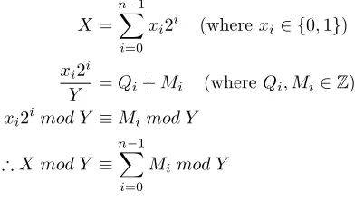
Because an integer represented in binary is made up of powers of 2s, it is said that the number is the sum of power of 2s. Therefore if we take the modulus of each power of 2 and sum them, it is equivalent to summing the power of 2s then taking the modulus, as shown in Theorem 2.
Theorem 2. Given an integer X, which is the sum of power of 2s, then the sum of the modulus’s of the power of 2s inY, is equivalent to the modulus ofX
Proof. GivenX mod Y whereX, Y ∈Z
X=
n−1
X
i=0
xi2i (wherexi∈ {0,1})
xi2i
Y =Qi+Mi (whereQi, Mi∈Z) xi2imod Y ≡Mi mod Y
∴X mod Y ≡
n−1
X
i=0
Mimod Y
Theorem 3 in the general context of the algorithm is the same as Theorem 1. However we require Theorem 3 because our proposed algorithm can use a lookup table (described in Section 4.1), which Theorem 1 does not make clear.
Theorem 3. Given an integerX, which is to be shifted bit left byw, the modulus of X bit shifted by w is equivalent to finding the modulus of X after being bit shifted.
Proof. Given (X << w)mod Y =M whereX, Y, M, w∈Z
Because left bit shifting X byw is equivalent to doubling X w times, we can use Theorem 1 to prove that:
((X mod Y)<< w) mod Y ≡(X << w)mod Y ≡M
The first 3 theorems are the basic underlying operations used in our al-gorithm. Now we need to prove the fundamental idea behind the alal-gorithm. Theorem 4 proves the initial step of the algorithm, splitting upX into elements of an array/vector so that they can be concatenated together to give X. Then when finding the modulus ofX, we can sum the modulus of each element (with bit shifting).
Proof. GivenX mod Y =M whereX, Y, M ∈Z
Y =
k−1
X
i=0
yi2i (whereyi∈ {0,1}andk >0)
X=
n−1
X
i=0
xi2i (wherexi∈ {0,1}andn mod k= 0)
ˆ X={
n−1
X
i=n−k
xi2i>>(n−k) !
, ... ,
k−1
X
i=0
xi2i !
}
Y =
k−1
X
i=0
yi2i (whereyi∈ {0,1}andk >0)
X≡
0
n
i=(n/k)−1
ˆ Xi
≡
(n/k)−1
X
i=0
( ˆXi<< ki)
Because the concatenation of ˆX is equivalent toX. Then by shifting each item in ˆX to the correct bit position and summing, is equivalent toX. Therefore we can use Theorem 2 and 3 so that
(n/k)−1
X
i=0
( ˆXi<< ki)mod Y ≡X mod Y
Note: ifn mod k6= 0 thenX can be padded with 0suntiln mod k= 0. Theorem 5 proves that a single precomputed value (or a lookup table), can be used to help find the modulus in each element greater than 0. This is an important property of the algorithm, as it allows the use of more precomputed values in the form of a lookup table.
Theorem 5. When calculating the modulus offXˆi in Y wherei >0, the mod-ulus is equivalent to multiplyingXˆi by 2kmod Y << k(i−1).
Proof.
ˆ
Xi<< ki mod Y
≡Xˆi2kimod Y
≡( ˆXimod Y)×(2kimod Y)
Instead of multiplying (as in Theorem 5), we instead shift each individual bit in an element and add if an overflow occurs. These are proven to be equivalent in Theorem 6.
Theorem 6. Left shifting Xˆi by ki in modulo Y where i >0, is equivalent to shifting Xˆi one shift at a time. Then if thekth bit becomes high after any shift (or add operation), drop it, and add 2k mod Y toXˆi. Therefore keeping the bit
width of Xˆi constant, while remaining in moduloY.
Proof.
ˆ
Xi×2ki mod Y
≡Xˆi<< ki mod Y
≡((( ˆXi<<1mod Y)...)<<1mod Y)
After each shift we put ˆX back into moduloY, and because ˆX haskbits, if the kth bit becomes high (i.e. overflow), we know that ˆX is definitely bigger than Y. Then by using Theorem 4 and 5, we can say that ˆX is equivalent in modulo Y to adding 2kmod Y to ˆX (after dropping thekth bit).
Theorem 6 is the main theorem for this algorithms operation (i.e. producing the correct answer). However for implementation, it would suffer from perfor-mance issues. This is due to the amount of shifting and potential adding which we would need to perform. So instead of shifting an element to its correct position directly, we can just shift it by the number of bits in Y, then start shifting the next element as well. This is shown in Theorem 7, and in terms of performance of the algorithm, is the most important theorem.
Theorem 7. If we start calculating the modulus of X in Y atXˆ(n/k)−1, then
instead of performing k(((n/k)−1)−1) number of shifts, we can perform k
shifts, then add Xˆ(n/k)−1 to Xˆ(n/k)−2. Repeating until we reach Xˆ0 which will
contain the result.
Proof.
ˆ
X(n/k)−1<< k((n/k)−2)
+Xˆ(n/k)−2<< k((n/k)−3)
≡ Xˆ(n/k)−1<< k << k((n/k)−3)
+Xˆ(n/k)−2<< k((n/k)−3)
≡ Xˆ(n/k)
−1<< k
+Xˆ(n/k)−2
3.4 Example
Below is an example on how to solve 1620mod11 on a 4-bit processor using our proposed algorithm.
1620 = 0110010101002
11 = 10112
ˆ
G= {01102, 01012, 01002}
T = ˆG[2] = 01102
T =T <<1 = 11002
T =T <<1 = 1 10002
T = 10002+ (100002mod10112)
= 10002+ 01012
= 11012
T =T <<1 = 1 10102
T = 10102+ 01012
= 11112
T =T <<1 = 1 11102
T = 11102+ 01012
= 1 00112
= 00112+ 01012
= 10002
T=T+ ˆG[1] = 10002+ 01012
= 11012
T=T <<1 = 1 10102
T= 10102+ 01012
= 11112
T=T <<1 = 1 11102
T= 11102+ 01012
= 1 00112
T= 00112+ 01012
= 10002
T=T <<1 = 1 00002
T= 00002+ 01012
= 01012
T=T <<1 = 10102
T =T+ ˆG[0] = 10102+ 01002
= 11102
T =T−11 = 11102−10112
= 00112
∴1620 mod 11=3
4
Implementation
4.1 Lookup Table
must be computed with the same modulo value, such as smart-cards or secure tunnels, there is a performance gain. The algorithm in its most basic form already uses a lookup table. For each shift, if an overflow occurs, we add a precomputed value, else we add nothing. This gives a simple lookup table as shown in Table 1.
Table 1.
Key Value
0 0
1 2kmod Y
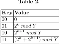
This can be extended to look at more bits at a time. For example, if we were to look at 2-bits, the lookup table would be that of Table 2.
Table 2.
Key Value 00 0 01 2kmod Y 10 2k+1mod Y 11 (2k+ 2k+1)mod Y
This allows us to shift by two bits at a time (instead of a single shift), but we still only require a single add. However this makes a software implementation slightly more difficult, because we cannot use the overflow bit anymore. Therefore we must look at the upper 2-bits of T before shifting. The current software implementation uses an and operation then a shift to get these upper bits. On a 64-bit processor, a lookup table with a key size of up to 64-bits, only requires the and and shift operations to be executed on a single 64-bit register, regardless of the size ofY. To possibly improve performance even more, one approach that could be explored is reversing the bits in each element (and keys), meaning only an and operation would be required.
4.2 Implementation Techniques
Using the algorithm proposed in Algorithm 4 for implementation on a standard processor can have some performance issues. This is because we are reliant on the number of bits inY. For example, if we are using a 64-bit processor, and we have Y which has 130-bits. Then X will be divided into elements of 130-bits, which is 2x64-bit registers (A and B), with the remaining 2-bits needs to go into another register (C). Then if we were to use a lookup table with a 4-bit key. We would need to combine the 2-bit value from register C, with the upper 2-bits of register B.
One solution to solve this is to round the number of bits inY up, so that it evenly divides the processors Arithmetic Logic Unit (ALU) width. In the example above, whereY had 130-bits, we would round it to 192-bits. This problem may also apply to custom hardware implementations, depending on the design. For example a smaller design may only use a 8-bit ALU, and could require Y to be rounded. But a design working on the full width of Y would not. Solving this problem is related to the design of the implementation, and this is just one proposed solution, of which they are many.
By rounding the bits inY, this means that our final answer can require more than one subtraction ofY
4.3 Memory Access
This algorithm has been designed in such a way that memory access has been kept to a minimum. Because the lookup table can be configured so that it can be stored in cache. Once it is loaded, the only memory access required is the data forX. Then since the algorithm only works on segments ofX at a time, it can load an element of X, process it, then load the next element. Therefore reducing the number of fetches (also cache misses), and improving performance. Each element loaded is the same number of bits asY, meaning ifY is 2048-bits, then the processor only needs to load 2048-bits at a time. This allows the data to be streamed into the processor, which is also important for a custom hardware implementation.
5
Comparisons
5.1 Comparisons with Barrett Reduction
Addition operations on large numbers are straight forward assuming the instruction set supports a carry bit. The words of the two input values can just added together. For example on Intel x86 processors, theadcinstruction can be used to add two words together, plus add a carry bit if an overflow occurred on the previous add or adc. Therefore if we are computing r=a+b, our pseudo assembly code would be
add r[0], a[0], b[0] adc r[1], a[1], b[1]
...
adc r[n], a[n], b[n]
where each word ofaandbare added together. Therefore the number of instruc-tions required is the number of words in the value. Subtraction can be achieved in a similar manner, by using thesub andsbb instructions.
Multiplication is not as simple as addition or subtraction, because each word in aneeds to be multiplied by all words in b. One technique to implement this is using basic long multiplication. For example if we are computing 33×52 on a 4-bit processor, we get
0010 0001
×0011 0100 1000 0100
+ 0110 0011 0000
0110 1011 0100
where we are only multiplying or adding 4-bits per cycle. Therefore in this exam-ple, we require 4 multiples, and 3 adds. This can get more complex if overflows occur when multiplying, often requiring more additions in modern instruction sets [2]. Scaling this up to multiplying two 2048-bit values on a 64-bit proces-sor, 1024 multiplications and even more additions depending on the amount of overflows that occur. Ignoring other instructions such as fetch, move and store, just this simple multiplication requires over 2048 instructions. The number of registers within the processor will also impact the performance because large numbers (i.e. 2048-bits) can be difficult to fit into registers all at once.
This is the disadvantage of using the Barrett reduction, because even though the operations used seem simple, in reality they can be complicated to imple-ment. The algorithm also makes use of the division operation which is more computationally intense than multiplication. However it depends on the value ofb.
and X is 2048-bits, therefore the main reduction is computed on the upper 1024-bits of X. Then the lookup table key can be 8-bits, resulting in a size of approximately 258Kb (1024-bit values + keys). This means that 1024/8 lookups are required. The bulk of the instructions are adding the lookup values each time. In this case, on a 64-bit processor, 2048 add instructions are needed. This is therefore comparable to a single multiplication in the Barrett Reduction (because the multiplication will be computed on 2048-bits). The shifts required will also require approximately 2048 instructions, which makes equals two multiplication operations. There are other instructions that will be required of course, like some additions for joining the elements together, and some final subtractions to get to the correct result. But these heavy depend on the inputted values.
At this point it is not possible to definitely claim our proposed algorithm is better than the Barrett Reduction. However by analysing the instructions required, we can show that it will use less instructions when compared to the Barrett Reduction, because of the Barrett Reductions heavy use of multiplica-tion and division instrucmultiplica-tions. Comparing implementamultiplica-tions of both algorithms in software is a difficult approach. Because both algorithms would be needed to be implemented fairly, with neither having any better code than the other (i.e. optimisations). Therefore only once a fully operational hardware implementation of our algorithm is complete, will we be able to provide a definite answer.
5.2 Comparisons with Montgomery Reduction
Unlike the comparison for the Barrett Reduction, comparing our proposed al-gorithm against the Montgomery Reduction is more straight forward. This is because the main operation used in Algorithm 2 is addition, which is the same as our proposed algorithm. Given that an addition in Algorithm 2 only occurs if a bit is high, we will say that on average, half of the bits are high. Meaning if the input is 2048-bits, only 1024-bits are high. Which therefore requires 1024 addi-tion operaaddi-tions. As discussed in the Barrett Reducaddi-tion comparison, one addiaddi-tion uses many instructions on a standard processor. Therefore on a 64-bit proces-sor, 16384 add instructions are required if the input is 2048-bit values. This is far more than our proposed algorithm would require, which was approximately 2048 add instructions, and approximately 2048 shift instructions, as shown in the Barrett comparison. The Montgomery Reduction also makes no guarantees on the number of bits required for each operation. For example, givenX mod Y, where X is 4096-bits and Y is 1024-bits, then each add operation will need to compute over 4096-bits. However our proposed algorithm will only compute over 1024-bits at a time. This is a very useful property for hardware implementations, and for making efficient use of registers and lower level cache.
proposed algorithm should allow for better implementations in both software and hardware over the Montgomery Reduction algorithms shown.
5.3 Comparisons with Fast Modular Reduction Method
This newly proposed algorithm in [5] is actually similar to the Montgomery Reduction in the sense that it looks at high bits. The difference is that it only processes the bits above bits of the modulus (Y), like our proposed algorithm. For example, givenX mod Y, whereX is 2048-bits andY is 1024-bits, then it will only process the upper 1024-bits ofX. Then for each high biti, it uses a lookup table to get the result of 2i mod Y and adds it to the result. Therefore if we again
say that half of the bits are high, 512 add operations are required. The bit width of the result is not clearly stated, however given that only values are added, it has to be 2048-bits (the same as X). Meaning at least 8192 add instructions would be needed, but will probably be closer to 16384. Our proposed algorithm would use far less instructions, and it guarantees the width of the result. Also because it keeps the result at a fixed width, the amount of subtractions required should be less on average, but this depends on the input.
Comparing the lookup tables, this algorithm [5] has a fixed size lookup table. So for example, if Y is 2048-bits, then there must be 2048 entries in the table, each of a size of 2048-bits. Resulting in a size of approximately 4Mb. Also because of this, the bit width of the inputX, can be no more than double the bit width of Y. This is because the lookup table only contains entries for the bits up to double that ofY, which for this example is 22048to 24096. This is a major limitation of this algorithm. However when looking at our lookup table, it can vary in size, and can support an arbitrary bit length of X. This is important to allow the table to fit in cache, and for devices which have limited storage. Using the same example where Y is 2048-bits, if the lookup table key is 8-bits, then the total size is approximately 0.5Mb. Our algorithm even allows for a lookup size of 1, if space is really limited.
Therefore our proposed algorithm is superior to that proposed in [5], both in terms of required instructions and the effectiveness of the lookup table. It is also a better option for hardware implementations because it can guarantee bit widths, and support varying sized lookup tables.
6
Performance Results
7919
10723 13171 41047 56003 0.6
0.8 1 1.2
Modulo Value
Seconds
(s) GMP
GMP Obtimised Proposed
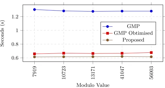
Fig. 1.2048-bitmod64-bit for 4000000 operations
The benchmarks were performed using an early 2013 MacBook Pro Retina 13”, which is equipped with a 2.6GHz Intel Core i5-3230M, 8GB 1600MHz DDR3, and a 128GB solid state drive. GMP was setup using both a default installation on Mac OS X using thebrew package manager [1], and an optimized configuration. GivenX mod Y, the benchmarks in Figure 1 use a 2048-bit value forX and a value within the first 10000 primes forY. Note that the results for our proposed algorithm include the time for computing the lookup table, which had a key size of 16-bits.
With the software implementation of our proposed algorithm still a work in progress. The current results shown in Figure 1 are more of a approximation of potential results instead of definite results. Therefore at this stage we cannot claim our software implementation is faster than GMP, even though early results are promising.
7
Future Work
The next step for this algorithm is to create an implementation on a Field-Programmable Gate Array (FPGA). Then to compare not only the performance, but also the area and power required, as well as looking into the effectiveness of side channel attacks. The current software implementation needs to be expanded to support an arbitrary length of input, for both X and Y. We also would like to experiment with compile time optimisations to give the algorithm better performance. This could lead to a large number library for software.
8
Conclusion
to be fetched. It is more advanced than other algorithms using lookup tables, such as in [5] and [11], because our algorithm allows the table to be used on an arbitrary input, while supporting a variable size. This is a truly unique property of our solution when compared to others. Our proposed algorithm could greatly impact the cyber-security landscape, by improving the performance of many security applications we use today.
References
1. Brew. Online http://brew.sh (Accessed 21/08/2014).
2. Intel 64 and ia-32 architectures software developer’s manual. Online http://www.intel.com/content/dam/www/public/us/en/documents/manuals/64-ia-32-architectures-software-developer-manual-325462.pdf (Accessed 27/08/2014). 3. Paul Barrett. Implementing the rivest shamir and adleman public key encryption algorithm on a standard digital signal processor. In Advances in cryptology— CRYPTO’86, pages 311–323. Springer, 1987.
4. Lejla Batina and Geeke Muurling. Montgomery in practice: How to do it more efficiently in hardware. In Topics in Cryptology—CT-RSA 2002, pages 40–52. Springer, 2002.
5. Zhengjun Cao, Ruizhong Wei, and Xiaodong Lin. A fast modular reduction method. IACR Cryptology ePrint Archive, 2014:40, 2014.
6. Joan Daemen and Vincent Rijmen. The design of Rijndael: AES-the advanced encryption standard. Springer, 2002.
7. Vincent Dupaquis and Alexandre Venelli. Redundant modular reduction algo-rithms. In Smart Card Research and Advanced Applications, pages 102–114. Springer, 2011.
8. Craig Gentry. Fully homomorphic encryption using ideal lattices. InSTOC, vol-ume 9, pages 169–178, 2009.
9. Burt Kaliski. Twirl and rsa key size. RSA Laboratories Technical Note, 2003. 10. Taek-Won Kwon, Chang-Seok You, Won-Seok Heo, Yong-Kyu Kang, and
Jun-Rim Choi. Two implementation methods of a 1024-bit rsa cryptoprocessor based on modified montgomery algorithm. InCircuits and Systems, 2001. ISCAS 2001. The 2001 IEEE International Symposium on, volume 4, pages 650–653. IEEE, 2001.
11. Chae Hoon Lim, Hyo Sun Hwang, and Pil Joong Lee. Fast modular reduction with precomputation. In Proceedings of Korea-Japan Joint Workshop on Information Security and Cryptology (JWISC’97), pages 65–79. Citeseer, 1997.
12. Chae Hoon Lim and Pil Joong Lee. Generating efficient primes for discrete log cryptosystems.
13. Peter L Montgomery. Modular multiplication without trial division. Mathematics of computation, 44(170):519–521, 1985.
14. Ronald Rivest, Adi Shamir, and Leonard Adleman. A method for obtaining digital signatures and public-key cryptosystems. Communications of the ACM, 21:120– 126, 1978.