Automatic Search of Attacks on round-reduced AES and Applications

(1)

Automatic Search of Attacks on round-reduced AES and

Applications

Charles Bouillaguet, Patrick Derbez, and Pierre-Alain Fouque

ENS, CNRS, INRIA, 45 rue d’Ulm, 75005 Paris, France

{charles.bouillaguet,patrick.derbez,pierre-alain.fouque}@ens.fr

Abstract. In this paper, we describe versatile and powerful algorithms for searching guess-and-determine and meet-in-the-middle attacks on some byte-oriented symmetric primitives. To demon-strate the strengh of these tools, we show that they allow to automatically discover new attacks on round-reduced AES with very low data complexity, and to find improved attacks on the AES-based MACs Alpha-MAC and Pelican-MAC, and also on the AES-based stream cipher LEX. Finally, the tools can be used in the context of fault attacks. These algorithms exploit the algebraically simple byte-oriented structure of the AES. When the attacks found by the tool are practical, they have been implemented and validated experimentally..

1 Introduction

Since the introduction of the AES in 2001, it has been questioned whether its simple algebraic structure could be exploited by cryptanalysts. Soon after its publication as a standard [NIS01], Murphy and Robshaw showed in 2002 an interesting algebraic property: the AES encryption process can be described only with simple algebraic operations in GFp28_q _{[MR02]. Such a result paved the way for multivariate}

algebraic techniques [CP02,Cid04] since the AES encryption function can be described by a very sparse overdetermined multivariate quadratic system overGFp2q. However, so far this approach has not been so promising [MV04,CL05], and the initial objective of this simple structure, providing good security protections against differential and linear cryptanalysis, has been fulfilled.

Recently, much attention has been devoted to the AES block cipher as a by-product of the NIST SHA-3 competition. The low diffusion property of the key schedule has been used to mount several related-key attacks [BKN09,BK09,BDK 10,KBN09] and differential characteristic developed for hash functions have been used to also improve single-key attacks [DKS10]. In order to find better attacks, new automatic tools have been designed to automatically search either related-key attacks or collision attacks on byte-oriented block ciphers [BN10] or AES-based hash functions [KBN09].

(2)

Related Work. In this security model, statistical attacks may be not the best possible attacks, since they usually require many pairs with specific input difference and algebraic attacks seem to be more well-suited. However, such attacks using either SAT solvers or Gr¨obner basis algorithms [MR02,BPW06], have never been able, so far, to endanger even very reduced versions of the AES even though its structure exhibits some algebraic properties. These attacks encode the problem into a system of equations, then feeds the equations to a generic, sometimes off-the-shelf equation solver, such as a SAT-solver or a Gr¨obner basis algorithm. The main obstacle in these approaches is the S-box, that only admits “bad” representations (for instance, it is a high degree polynomial over the AES finite field), and increases the complexity of the equations, even though low degree implicit equations may also exist.

Our tools, instead of using pre-existing generic equations solvers, first run a search for an ad hoc solver tailored for the equations to solve, build it, and then run it to obtain the actual solutions. They can be applied to systems of linear equations containing a non-linear permutation of the field, such as an S-box. Our idea is to consider the S-box as a black box permutation. We only use few properties of this function and our attacks works forany instantiation of the S-box.

This approach is reminiscent of the ideas used by Khovratovich, Biryukov and Nicoli´c to find collisions in an AES-based hash function (more precisely, a hash function using a large version of Rijndael in Davies-Meyer mode) [KBN09]. They first found a “good” colliding truncated differential path, and they were facing the problem of finding a conforming pair to obtain an actual collision. The basic strategy for finding a message pair conforming to a differential path consists in exhaustively trying all possible input values and checking if the constraints are satisfied. In order to speed up the collision search, these authors used a message modification technique: they described the hash function using a system of linear equations with an S-box, and added equations to enforce that the message and chaining value follow their truncated differential characteristic inside the function. Solving the equations would yield a collision, and the approach they proposed is to look automatically for constraints that could be satisfied by setting a particular variable to a particular value without violating other constraints. To this end, they use linear algebra, and essentially consider xand Spxqto be independent variables, and then greedily satisfy constraints. This method is however limited in that when the greedy strategy aborts,i.e., when no easily-satisfiable constraints remain, then probabilistic trials is the only fallback.

Our Techniques and Results. Our tools try to find attacks automatically by searching some classes of guess-and-determine and meet-in-the-middle attacks. They take as input a system of equations that describes the cryptographic primitive and some constraints on the plaintext and ciphertext variables for example. Then, it solves the equations by first running a (potentially exponential) search for a customized solver for the input system. Then, the solver is run, and the solutions are computed.

We describe two tools. Our preliminary tool uses a depth-first branch-and-bound search to find “good” guess-and-determine attacks. It has been (covertly) used to generate some of the attacks found in [BDD 10], and outperformed human cryptanalyst in several occasions. However, the class of attack searched for by this preliminary tool is quite restricted, and it fails to take into account important differential properties of the S-box. Our second, more advanced tool, allows to find more powerful attacks, such as Meet-in-the-Middle attacks. For instance, it automatically exploits the useful fact that an input and output difference on the S-box determine almost uniquely the actual input and output values. The algorithmic techniques used by this tool are reminiscent of the Buchberger algorithm [Buc65]. The results found by these algorithms are summarized in tables 1 and 2.

We improve many existing attacks in the “very-low data complexity” league. For instance, we find a certificational attack on 5 AES rounds using just a single known plaintext, and a practical attack on 4 full AES rounds with 4 chosen plaintexts. We also look at AES-based primitives. We independently discovered (along with [DKS11]) the best known attack on Pelican-MAC, and automatically rediscover the best attacks on Alpha-MAC and LEX. We also used our tool to find a new, faster, attack on LEX. Lastly, we improve the efficiency of the state-recovery part of the Piret-Quisquater fault attack against the full AES. While it required 232 _{elementary operations, it now takes about one second on a laptop.}

Since most of the attacks we present are practical, or have a practical core, we implemented many of them and tested them in practice. The source code of some of these attacks is available at:

http://www.di.ens.fr/~bouillaguet/implementation.html

(3)

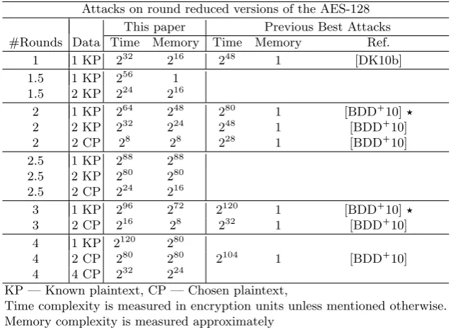
Attacks on round reduced versions of the AES-128

This paper Previous Best Attacks

#Rounds Data Time Memory Time Memory Ref.

1 1 KP 232 ₂16 ₂48 ₁ _[DK10b]

1.5 1 KP 256 ₁

1.5 2 KP 224 216

2 1 KP 264 248 280 1 [BDD 10]

2 2 KP 232 ₂24 ₂48 ₁ _{[BDD 10]}

2 2 CP 28 28 228 1 [BDD 10]

2.5 1 KP 288 288

2.5 2 KP 280 280

2.5 2 CP 224 ₂16

3 1 KP 296 ₂72 ₂120 ₁ _{[BDD 10]}

3 2 CP 216 28 232 1 [BDD 10]

4 1 KP 2120 280

4 2 CP 280 ₂80 ₂104 ₁ _{[BDD 10]}

4 4 CP 232 224

KP — Known plaintext, CP — Chosen plaintext,

Time complexity is measured in encryption units unless mentioned otherwise. Memory complexity is measured approximately

: previously published, but found with these tools “r.5 rounds” —rfull rounds and the final round

Table 1.Summary of our Proposed Attacks on AES-128

finder in section 3 and then a more advanced tool that finds meet-in-the-middle attacks in section 4. Finally, in sections 5, 6 and 7, we show several attacks that were automatically found by the previous tool.

2 Description of the AES

The Advanced Encryption Standard [NIS01] is a Substitution-Permutation network that supports key sizes of 128, 192, and 256 bits. A 128-bit plaintext (resp. a 128-bit key or internal state) is treated as a byte matrix of size 44, where each byte represents a value inF28. An AES round applies four operations

to the state matrix:

– SubBytes(SB) — applying the same 8-bit to 8-bit invertible S-box 16 times in parallel on each byte of the state,

– ShiftRows (SR) — cyclic shift of each row (thei’th row is shifted byi bytes to the left), – MixColumns (MC) — multiplication of each column by a constant 44 matrix overF28, and

– AddRoundKey (ARK) — XORing the state with a 128-bit subkey.

Fig. 1An AES round

0 4 8 12 1 5 9 13 2 6 10 14

3 7 11 15 3 7 11 15 15 3 7 11

ShiftRows MixColumns

SB SR MC ARK

L

ki

xi yi

zi wi

Hello, here is some text without a meaning. This text should show, how a printed text will look like at this place. If you read this text, you will get no information. Really? Is there no information? Is there a difference between this text and some nonsense like≫Huardest gefburn≪.

Kjift – Never mind! A blind text like this gives you information about the selected font, how the letters are written and the impression of the look. This text should contain all letters of the alphabet and it should be written in of the original language. There is no need for a special contents, but the length of words should match to the language.

(4)

Attacks on Primitives based on AES

Primitive Complexity G & D Part References

Data Time Memory Time Memory

Pelican-MAC 285.5 queries 285.5 285.5 [YWJ 09]

Pelican-MAC 264_queries ₂64 ₂64 ₂32 ₂24 _{Sect. 6}

Alpha-MAC 265_queries ₂64 ₂64 ₂32 ₂16 _{[YWJ 09]}_:

LEX 236.3 _bytes ₂112 ₂36 _[DK08]

LEX 240bytes 2100 264 280 1 [DK10a]

LEX 236.3 _bytes ₂96 ₂80 ₂64 ₂64

LEX 250bytes 280 248 216 28 Sect. 7.2

AES-128 1 fault 232 232 232 232 [PQ03]

AES-128 1 fault 224 216 224 216 Sect. 5.3

Time complexity is measured in encryption units unless mentioned otherwise. Memory complexity is measured approximately

:: the tools can find automatically a comparable attack

Table 2.Summary of our Proposed Attacks on Primitives based on AES

number of rounds depends on the key length: 10 rounds for 128-bit keys, 12 rounds for 192-bit keys, and 14 rounds for 256-bit keys. We use the round numbers 1, . . . , N r, where N r is the number of rounds (N rP t10,12,14u). We only consider the AES with 128-bit keys and 10 rounds. Because the final AES round is different from the others, we use the term “r.5 rounds AES” to denote the AES reduced topr 1q rounds, including the final round. We use “r rounds AES” to denote the AES reduced tor identical full rounds. In our terminology, the “normal” 128-bit AES has 9.5 rounds.

LetF28 be the finite field with 256 elements used in the AES. We represent the S-box of theSubBytes

transformation byS:F28 Ñ_F₂8. In a 44 matrix, we use the following numbering of bytes: byte zero

is the top-left corner, the first column is made of bytes 0-3, while the last column is made of bytes 12-15, with byte 15 in the bottom-right corner (this is illustrated by Figure 1). We denote the four columns of a 44 matrixM byMr0..3s, Mr4..7s, Mr8..11sandMr12..15srespectively.

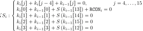
As we consider only the AES with 128-bit key, we shall describe only its key schedule algorithm. The key schedule of the other variants can be found in [NIS01]. The key schedule of AES-128 takes the 128-bit master key k0 and extends it into 10 subkeys k1, . . . , k10 of 128 bits each using a key-schedule

algorithm given by the following equations:

KSi : $ ' ' ' ' & ' ' ' ' %

kirjs kirj4s ki1rjs 0, j4, . . . ,15

kir0s ki1r0s Spki1r13sq RCONi 0 kir1s ki1r1s Spki1r14sq 0

kir2s ki1r2s Spki1r15sq 0

kir3s ki1r3s Spki1r12sq 0

We denote by xi the internal state entering roundi (i.e., beforeSubBytes), byyi the internal state between theSubBytesandShiftRows operations, whilezi andwi denote the internal state before and after theMixColumns operation, respectively. The plaintext is denoted by P, and the ciphertext byC. One round is represented by these equations:

Ri: $ ' ' ' ' ' ' & ' ' ' ' ' ' %

yi Spxiq 0

wi

02 03 01 01 01 02 03 01 01 01 02 03 03 01 01 02

yir0s yir4s yir8s yir12s yir5s yir9s yir13s yir1s yir10syir14s yir2s yir6s yir15s yir3s yir7s yir11s

0

xi 1 wi k1 i0

It is straightforward to form the system of equationsEdescribing the full encryption process along with

the key schedule: we just have to concatenate someKSi’s and someRi’s (without forgetting the initial key addition). Since the right-hand side of all these equations are zero, we stop representing it from now on.

(5)

Let us denote byVpXqthe vector space spanned by 1, x, Spxqfor allxPX, for any set of variablesX. We denote by X the set of all key and internal state variables, and then the cipher equations span a

subspace ofVpXq. Any basis of this subspace describes an equivalent system of equations. Therefore, by

an abuse of notation we identify the set of equations describing the block cipher with the vector space formed by all the linear combinations of the equations, and we still denote it by E. We also introduce

the notationSp_Eqto denote the set of solutions of the equationsEandOpEqto denote their number.

In some cases, we are interested in interchanging the order of the MixColumns and AddRoundKey

operations. As these operations are linear they can be interchanged, by first XORing the data with an equivalent key and only then applying the MixColumnsoperation. We denote the equivalent subkey for the altered version by:

ui M C1pkiq

0e 0b0d09 09 0e0b 0d 0d09 0e0b 0b0d09 0e ki

3 A preliminary Tool for Simple Guess-And-Determine Attacks

Confronted with a system of equations inVpXq(possibly describing a cryptographic problem), the most

naive way to obtain its solutions consists in enumerating all the possible values of the variables and retaining only the combinations satisfying all the equations. However, equations inVpXqare such that,

in a given equation, once all the terms but one are known then the value of the last one can be found efficiently. This is especially useful when the equations are sparse (efficient cryptographic primitives usually result in sparse equations). This enables more or less efficientguess-and-determine techniques to solve the equations. In a cryptographic setting, guess-and-determine attacks are often found when data is very scarce, and statistic attacks are therefore impossible. Guess-and-determine attacks can be more or less sophisticated, but the simplest ones typically take the following form:

1: for allvalues of some part of the (unknown) internal statedo

2: Compute the full internal state

3: Retrieve the secrets

4: Check the secrets against available data

5: if match then returnsecrets

6: end for

The difficulty in finding such an attack is to find which parts of the internal state to enumerate, and how to recover the rest. In this section, we present a preliminary tool that finds such attacks automatically. It takes as input a system of equations E VpXq and a set K0 X of initially known variables—

these are the variables corresponding to the available data, for instance the plaintext, the ciphertext, the keystream, etc. The preliminary tool returns a C++ function (the “solver”) which enumerates the solutions ofE (using negligible memory), given the actual values of the known variables. The tool also

returns the exact number of elementary operations the solver performs in the worst case.

This preliminary tool has been developed while performing the research that led to the results pub-lished in [BDD 10]. The preliminary tool has for instance been used to findone known plaintextattacks against 1, 1.5, 2, 2.5 and 3 AES rounds, systematically beating the best results found manually. For instance, prior to the publication of [BDD 10], the best attack on one (full) AES round was a guess-and-determine attack with complexity 248_{described in [DK10b]. The preliminary tool found in less than}

a second an attack of complexity 240 _{and generated its implementation. This attack runs as expected in}

about 18 hours using 8 Intel Xeon E5440 cores at 2.83GHz (the parallelization is straightforward using OpenMP).

3.1 Knowledge Propagation

The core idea of this preliminary tool is quite simple: if there is a linear combination of the equations in which the values of all terms are known except one, then the value of this last term can be determined efficiently.

(6)

An “algebraic” Point of View. The acquisition of further knowledge, either by “guessing” or “deter-mining” the value of a variable has a simplifying effect on the equations (it removes an active variable whose value is unknown from the problem). This simplification of the original equations in fact has a clean algebraic description.

Let K X be a set of variables whose values are known. If we substituted the values of known

variables into the original equations E, we would indeed get a system with less variables. In fact, this

reduced system is essentially the subspacepE VpKqq{VpKqof thequotient spaceVpXq {VpKq: starting

from an equation f PE, its equivalence class rfsin the quotient contains a representative where all the

variables in K have disappeared. Alternatively, the variable x can be deduced fromK if either rxs or

rSpxqsbelong to the quotient of E VpKq byVpKq, and we will writexPPropagatepKq when it is

the case. To see why, observe that rxs P pE VpKqq{VpKq (resp. rSpxqs P pE VpKqq{VpKq) means

that there exist k P Vp_Kq such that x k P E (resp. Spxq k PE). In other terms, there is a linear

combination of the equationsEthat can be writtenx k(respectivelySpxq k). It follows that in any

solution of the equationsE, the value ofx(resp.Spxq) is the value ofk. There is therefore a straight-line

program of sizeOp|K|qthat uniquely determines the value ofxgiven the values of the variables inK—it

just has to evaluatek.

Observe in passing that it is not difficult to check whether x PPropagatepKq: it comes down to

solving a system of (at most) 2|X|linear equations in|E|variables overF28.

3.2 Automatic Search For a Minimal Number of Guesses

Given a set of “known” variables K0, we may propagate knowledge and obtain the value of new

vari-ables, yielding a new set of known variablesK1. But it may turn out that new variables may again be

obtained fromK1. We therefore define the functionPropagatepXqwhich returns the least fixed point

ofPropagatecontainingX:

PropagatepXq

"

let Y PropagatepXqin

if XY then return Y else return _PropagatepYq

Note that this definition is well-founded, because Propagate is both monotonic and bounded. In-deed, it is very easy to check that X Y implies PropagatepXq PropagatepYq. It follows that Propagate is monotonic as well.

A guess-and-determine solver has been found as soon as we have found a setGof “guesses” such that

PropagatepGq X. In that case, we will say that G issufficient. The problem thus comes down to

automatically finding a sufficient set of minimal size.

The process of exhaustively searching such a set of variables to guess can be seen as the exploration of a Directed Acyclic Graph (DAG) whose nodes are sets of variables. The starting node is the setK0, and

the terminal node isX. For any set of variablesX, and any variableyRXthere is an edgeX ÝÑy XYtyu,

meaning that we may always choose to “guess” the value of y to gain knowledge. Finally, for any set of variablesX, there is an edgeX ÑPropagatepXq, symbolizing the fact that increase we may increase our knowledge by propagation.

In this setting, the preliminary tool tries to find a path fromK0toXgoing through a small (if not the

smallest) number of “guess” edges. Indeed, the cost of the resulting attack is exponential in the number of “guessed” bytes. The problem is that the size of the DAG is exponential in the number of variables.

The search works in a depth-first branch-and-bound fashion reminiscent of the DPLL procedure implemented in many SAT-solvers. The pseudo-code of the search procedure is shown in Algorithm 1. The functionExplorepK,G,Bqreturns a minimal set of variables to guess in order to be able to recover

the entire internal state. HereKdenotes the set ofcurrently knownvariables (i.e., the current node of the

DAG),Gdenotes the set of variables that have been guessed so far, andBdenotes the set of variables that

have been guessed in the best previously known solution. This implicit assumption is that|G| |B|, and

that the result of Explorehas cardinality smaller than or equal to B. EvaluatingExplore(K0,H,X)

returns a minimal solution.

3.3 Pruning Strategies

(7)

Fig. 2The possible sets of guessed variables explored by the tool to find an attack one full AES round. Each descendant has one more guess than its parent.

root

Algorithm 1Pseudo-code of the Preliminary Tool

1: functionExplore(K,G,B) 2: if KXthen returnG 3: if KPropagatepKqthen

4: returnExplorepPropagatepKq,G,Bq 5: if |G| |B| 1then returnB

(8)

used severalpruning strategies that remove “guess” edges from the DAG without modifying its reacha-bility properties. These pruning strategies appear in Algorithm 1 under the form of theFilterGuesses function, which only returns a subset of its argument.

Local Pruning. When it is necessary to guess a new variable, we have to choose which new variable to guess. Some choices may beequivalent (i.e., yield the exact same knowledge after Propagate), while some choices may besuperior to some others: if guessing the value ofxallows to deduce the value ofy, then it is always better to guessxinstead ofy. Indeed, we see that ifyPPropagatepKY txuq, then:

PropagatepKY tyuq PropagatepKY txuq

Given a set of known variables, this translates to a partial quasi-order relation on variables:

x¥_KyðñyPPropagatepKY txuq.

This quasi-order in turn induces an equivalence relation between variables:

x_K yðñ px¥_Kyqandpy¥_Kxq

It is easy to check thatxKy means that guessingxis equivalent to guessingy. Indeed, we have:

xKyðñPropagatepKY txuq PropagatepKY tyuq PropagatepKY tx, yuq.

It is therefore sufficient to guess only one variable per equivalence class. In addition, the quasi-order induces a strict partial quasi-order (which we denote by¡K) on the setΩpKq X{K of all equivalence

classes. In fact,x¡K ymeans that any guess in the class ofxyields more knowledge that a guess in the class ofy. It is indeed easy to check that:

x¡KyùñPropagatepKY tyuq PropagatepKY txuq

As a consequence, an interesting pruning strategy consists in trying to guess only one variable per maximal equivalence class (for ©K) from a node labelled by K. We call this strategy “local pruning” because it only requires a local exploration of the DAG around the current node.

LetG pV, Eqdenote the DAG defined in section 3.2, and letG1 denote the “locally pruned” DAG (in fact it is a subgraph ofG). Letρdenote a function that maps equivalence classes to their canonical representative (for instance, the variable with the smallest index), and let ΩmaxpKq denote the set of

maximal equivalence classes:

ΩmaxpKq

!

XPΩpKq : @Y PΩpKq, Y £KX )

.

ThenG1 pV, E1qwhere E1 E only contains the following edges:

KÑPropagatepKq for allKX

KÝÝÝÑρpXq KY tρpXqu for allKX, X PΩmaxpKq

We now argue that this is a valid pruning strategy. We first prove an (easy) technical lemma.

Lemma 1. If there is a path from any node Kto Xin G(resp. G1) that crosses k“guess” edges, then

there is a path inG(resp.G1) from any superset ofKtoXthat crosses at mostk“guess” edges.

Proof. Let us denote byX an arbitrary superset of K. We prove the result by induction on the length

of the path. IfKX, then there is nothing to prove. Otherwise, there are several cases to consider.

i) The first edge of the path isKÑPropagatepKq, and there exist an edgeXÑPropagatepXq. In this case, PropagatepXqis a superset ofPropagatepKq, and by induction hypothesis there

exist a path with at most kguess edges betweenPropagatepXqandX. It is easy to conclude.

ii) The first edge of the path isKÑPropagatepKq, and there is no edgeXÑPropagatepXq. In this case,X PropagatepXq, and the previous argument can be adapted, sinceX is a superset ofPropagatepKq.

iii) The first edge of the path isKÝÑx KYtxuandxPX. This case is easy, asX is a superset ofKYtxu,

(9)

iv) The first edge of the path isK ÝÑx KY txuand xR X, but the edge X ÝÑx X Y txu exists in the

graph. Then, becauseXY txuis a superset ofKY txu, we can conclude by induction that there is

a path in the graph with at mostk1 edges betweenXY txuandX.

v) Lastly, the first edge of the path is K ÝÑx KY txu and xR X, but the edge X ÝÑx X Y txu does

not exist in the graph. This situation only occur in the “pruned” graph. However, there exist by definition an edge X ÝÑy X Y tyu such that PropagatepX Y txu PropagatepXY tyuq. It follows that PropagatepXY tyuq contains bothX andx, and is therefore a superset ofKY txu.

We can then conclude by induction.

We are now ready to state that pruning the graphGcannot accidentally kill the best solutions. Lemma 2. If there is a path from any node _Kto _X inG that crosses k“guess” edges, then there is a path from KtoXinG1 that crosses at mostk“guess” edges.

Proof. The proof is by induction on the total number of edges in the path betweenK and X in G. If KX, then there is nothing to prove. Otherwise, if there is a “propagate” edge going out of K, then

there exists a path in Gfrom PropagatepKq to Xthat crosses at most k guess edges. By induction

hypothesis, a path of lower cost exists inG1, and the edgeKÑPropagatepKqalways exist inG1.

If there are only “guess” edges going out ofK, then we denote the first edge of the path fromKtoX

inGbyKÝÑy KY tyu, and byY the class ofy. Two cases are possible:

– Either Y is maximal (i.e., belongs to ΩmaxpKq), and there is an edge K

ρpYq

ÝÝÝÑ KY tρpYqu in G1.

By definition, we know that PropagatepKY tyuq PropagatepKY tρpYquq. It follows that

there is a path in G with at most k1 guess edges from PropagatepKY tρpYquq to X, which

allows to conclude by induction hypothesis that a corresponding path also exists in G1. Because PropagatepKY tρpYquq is reachable inG1 fromK, the result is established.

– OrY is not maximal, which means that there is another classXPΩmaxpKqsuch thatX ¡KY. Then in G1 there is an edge K

ρpXq

ÝÝÝÑ KY tρpXqu. Because PropagatepKY tyuq PropagatepKY

tρpXquq, then there is inGa path with at mostk1 guess edges betweenPropagatepKYtρpXquq

and X(this is guaranteed by lemma 1), and by induction hypothesis a corresponding path exists in

G1. From there, it is easy to see that there is a path from K to X(via KY tρpXqu) in G1 with at

mostkguess edges. [\

Global Pruning. A somewhat surprising consequence of the fact thatPropagateismonotonicbrings in a interesting result, enabling us to further discard some bad guesses in a very powerful way.

Lemma 3. Let V Xbe an insufficient set of variables, and let GXbe a sufficient set of variables.

Then:

GX pXPropagatepVqq H

Proof. Let us reason by contradiction and assume thatGX pXPropagatepVqq H. Then, because

Gis a subset of X, thenGPropagatepVq. By monotonicity and idempotence of Propagate we

find:XPropagatepGq PropagatepVq X. [\

IfGis a sufficient set of minimal size, then Lemma 3 gives usa priori knowledge onG, and it enables

to choose the first guess of the search procedure inXPropagatepVqwithout risking to throw the best solution away.

It is possible to exploit lemma 3 even further for more pruning. Let us assume that in the explo-ration process we currently know the variables in K, and that we have guessed the variables in G, so

that KPropagatepGq. LetB be a sufficient set of minimal size such thatGB,i.e., the best we

may hope to find from the current state. Lemma 3 tells us thatBX pXPropagatepVqq H. This reveals us some variables inB, and could be used to direct the exploration towards B. However, ifV is

badly chosen then it may very well be that all the interesting variables we learn to be in Barealready

known, in which case we would not learn anything.

However, choosing V to be a superset ofKensures thatKX pXPropagatepVqq H, and thus removes the previous problem. We may safely choose our next guess inXPropagatepVqwhenKV.

(10)

Algorithm 2Pruning Strategies for Algorithm 1.

1: functionGreedyGlobalPruning(V)

2: Find variablexPXV such that|PropagatepV Y txuq|is minimal

3: if PropagatepV Y txuq Xthen returnV 4: returnGreedyGlobalPruningpV Y txuq

5: end function

6: functionLocalPruning(K, V)

7: BadÐ H

8: for allxPV do

9: if xRBadthen

10: for allyPPropagatepKY txuqdo

11: if yxthenBadÐBadY tyu

12: end for

13: end if

14: end for

15: returnV Bad

16: end function

17: functionFilterGuesses(K)

18: CandidatesÐGreedyGlobalPruningpKq 19: for allxPCandidatesdo

20: if there existyPGsuch thatx XythenCandidatesÐCandidates txu 21: end for

22: returnLocalPruning(Candidates) 23: end function

Linearly Occurring Variables. Since the equations E cannot be completely linear—unless we were

looking at a very uninteresting primitive—, then some variables appear both linearly, and under the S-box. However, some variables may appear only linearly (this is for instance the case of the last round key in the AES). If a variablexoccurs only linearly, then it can be eliminated from all the equations except one by taking linear combinations of the equations. Taking apart the single equation containingx, we obtain a new system of equationsE1 with one less equation and one less variable. The search procedure

can safely be run onE1.

3.4 Computing and Testing Solutions

If xi P PropagatepKq, then there exists a vector αi such that rEαis rxis (resp. rSpxiqs), where

the square brackets again denotes the equivalence class in the quotient E{VpKq. The vectorαi can be

computed using straightforward linear algebra given xi and K, as mentioned in section 3.1. Once a

sufficient setGhas been found, and all the vectors αi have been computed, we consider the subspaceP

spanned byEαi for all vectorsαi corresponding to “propagated” variables inXG. All the equations

belonging to this subspaceP are satisfied by definition once the variables inXGare “determined” from

those (inG) whose values have been guessed.

It is therefore interesting to consider a supplementary C of P in E: it describes equations that are

(linearly) independent from those used for the “determine” step of the attack. To check whether a given choice of values for the guessed variables is correct, it suffices to a) determine the values of the other variables and b) check whether the equations in C hold. The complexity of the resulting procedure is roughly 256|G| _encryptions.

3.5 Implementation Details

Writing a proof-of-concept implementation of Algorithm 1 is not very complicated, but writing anefficient version thereof is a bit more challenging. The only non-trivial parts in the implementation of the search procedure is the data structure holding the equationsEand thePropagatefunction. To make it efficient, we exploited the sparsity of the equationsE. Recall from section 3.1 thatPropagatetries to solve the equation inα:

rEαs rxs (1)

(11)

triangular solver with sparse right-hand-side,i.e., a sparse linear algebra subroutine that solvesAxy whenAis triangular and sparse, andyis also sparse. The interest of this procedure is that it may perform sensibly less thannoperations whenAandy are sparse enough (see [Dav06] for more details).

The quotient operation in fact removes rows from the matrices and the vectors it is applied to. So, when a new variable x becomes “known”, we have to remove the rows x and Spxq from the matrix representing the equations. If one of these rows was pivotal, then removing it may leave the matrix in a non-echelonized state. This can be fixed through a simple column permutations in some cases. In some other cases, a new column has to be recomputed, using a variant of the sparse triangular solver. All in all, removing rows and re-echelonizing the matrix represent a negligible fraction of the running time, because the matrix representing E is stored in a special sparse data-structure: non-zero entries

are stored column-wise and row-wise in doubly-linked lists. This allows to efficiently remove rows and columns. Removed entries are kept in memory, and can be efficiently restored when backtracking. An array stores the pivot column for each (pivotal) row. A useful optimization follows from the observation that equation (1) only has a solution ifx(resp.Spxq) is a pivotal row in the matrix.

The code has been written in the OCaml language, and weights about 5000 lines, more than 1500 of them devoted to the linear algebra. Debugging the sparse linear algebra subroutines was a bit chal-lenging because of the unusual data-structure holding the matrix. Parallelizing the DAG exploration is not difficult, and we developed a distributed version of Algorithm 1 using a customized version of the MapReduce framework [DG10] built on top of Leroy’s OcamlMPI library (and building on ideas by Filliˆatre and Kalyanasundaram [FK11]). We used it to run our program on two types of platform:

– Roughly 100 Intel cores of various speeds (between 2 and 3 Ghz) in parallel using all the desktop computers of the lab during the night.

– 400 MIPS-like cores in a server containing 8 Tilera TilePRO64 CPUs with 50 available cores each (unfortunately, the OCaml compiler cannot generate native MIPS assembly, and hence generated bytecode. Interpreting the bytecode causes a tenfold performance penalty).

On the second platform, exploring the graph for one full round takes about a minute. For 1.5 rounds, it takes 18 minutes (and finds an attack with 7 guessed bytes). For 2 full rounds, it takes 67 minutes. For 2.5 rounds, it takes 3 weeks. We did not have the patience to wait a few weeks for the exhaustive search to terminate on 3 rounds (a solution faster than exhaustive search was found, but we have no guarantee that it is the fastest attack of the considered class). At the very least, we hope that we demonstrated that it is possible to parallelize the search process at will.

3.6 Limitations

The main limitation of this approach is that it completely fails to take into account the differential properties of the S-box. For instance, it cannot exploit the fact that when the input and output differences of the S-box are fixed and non-zero, then at most 4 possible input values are possible. Therefore, this approach alone does not bring useful result when more than one plaintext is available. However, it can be used as a sub-component in a more complex technique. We now move on to describe such a generalization that allows to find more powerful attacks.

4 An Improved Tool for Meet-In-The-Middle Attacks

The equations describing the AES enjoy an interesting and important property. Let us consider a cover of the set of variables,XX1YX2 (the intersection ofX1andX2may be non-empty). Then any equation

f PEcan be writtenf f1 f2, with f1 PVpX1qand f2PVpX2q. In some sense, these equations are

separable. We will see that this allows a recursive meet-in-the-middle approach.

4.1 Solving Subsystems Recursively

The simple algebraic structure of the equations allows us to efficiently extract from a systemEasubsystem

containing only certain variables (sayX1), by simply computing the vector space intersectionEXVpX1q.

In the sequel we will denote it by EpX1q. We note that a solution ofE is also a solution ofEpX1q, for

anyX1X, but that the converse is not true in general.

Now let us be given a partitionXX1YX2(we first study the caseX1XX2 H) and twoblack-box

(12)

two sub-solvers A1 and A2 to find the solutions SpEq of the full problem. An obvious way would be

to compute the solutions S1 of EpX1q and S2 of EpX2q, and to test all the solutions in the Cartesian

productS1S2. This would require checking|S1| |S2|candidates against the equations.

It is possible to do better though. Firstly, we observe that the vectors inS1S2automatically satisfy

the equations inEpX1q EpX2q. Therefore we first compute a supplementary ofEpX1q EpX2qinsideE

(let us call itM). The solutions ofEare in fact the elements of S1S2satisfying the equations of M.

This already makes less constraints to check. Second, sieving the elements satisfying constraints from M can be done in roughly|S1| |S2|operations, using variable separation and a table. Let pfiq1_¤i¤m be a basis ofM, andfi gi hi withgiPVpX1qandhi PVpX2q. If the values of all the variables in X1 (resp.X2) are available, then the gi’s (resp. hi) may be evaluated. We denote by G (resp. H) the

function that evaluates all thegi (resp.hi) on its input. If` |X1|, then:

G:px1, . . . , x`q ÞÑ

g1px1, . . . , x`q, . . . , gmpx1, . . . , x`q

We build two tables:

L1ÐÝ tpGpx1q, x1q | x1 solution ofEpX1qu

L2ÐÝ tpHpx2q, x2q | x2 solution ofEpX2qu

Then, the solutions ofEare the pairspx, yqfor which there exist azsuch thatpz, xq PL1andpz, yq PL2.

They can be identified efficiently by various methods (sorting the tables, using a hash index, etc.). We have just combined A1 and A2 to form a new solver, AA1 'A2, that enumerates the solutions of E. Note that to extend this work at a cover ofX we just have to perform the match also on variables

common toX1and X2.

Complexity of the Combination. Given a cover X X1 YX2, and two sub-solvers A1 and A2

respectively computingSp_Ep_X1qqandSpEpX2qq, the complexity and the properties ofAA1'A2 are

easy to determine. Let us denote by TpAqthe running time of A, byMpAq its memory consumption, and by VpAq the set of variables occurring in the corresponding equations. The number of solutions returned by a solverAonly depends onVpAq, as it is the number of solutions ofEpV pAqq. For the sake

of simplicity, we denote it byOpAq, and for that of consistency we also use the notation OpEpV pAqqq.

Note that the number of solutions found by a solver cannot be greater than its running time, so that OpAq ¤TpAq.

The number of operations performed by the combination is the sum of the number of operations produced by the sub-solvers plus the number of solutions (the time required to scan the tables, namely |S1| |S2|, is in the worst case of the same order as the running time of the two sub-solvers), so that

TpA1'A2q TpA1q TpA2q O

A1'A2 .

However, we use the following approximation

TpA1'A2q max

!

TpA1q, TpA2q, O

A1'A2

) .

It is possible to store only the smallest table, and to enumerate the content of the other “on the fly”, while looking for a collision. This reduces the memory complexity to the maximum of the memory complexity of the sub-solvers, and the size of the smaller table. This yields:

MpA1'A2q max

!

MpA1q, MpA2q,min

OpA1q, OpA2q

) .

Heuristic Assumption On the Number of Solutions. Evaluating the complexity of a given (possibly recursive) combination requires evaluating the number of solutions of various sub-systems. This is a difficult problem in general, and in order to be able to quickly evaluate the properties of a combination, we use the followingheuristic assumption:

log256OpEpXqq |X| dimEpXq.

(13)

this assumption holds. A difficulty that we encountered in practice stems from the following “differential”

system: _"

x y∆i

Spxq Spyq ∆o .

IfS is the S-box of the AES, then this system has one solution on average (over the random choice of the differences), and the hypothesis holds. However, in degenerate situations, for instance when∆i ∆o0, then the system has 28_{solutions... Surprisingly, an S-box with very bad differential properties would make}

life more difficult for our tool. This follows from the fact that on a good S-box, there are very few pairs of input/output values that generate a given input/output difference, and this makes our assumption more likely to hold in “differential” situations.

This assumption makes it easy to evaluate the performance of the combination of two sub-solvers: it boils down to computing the dimensions of a few vector spaces.

In addition, it provides this interesting property:

Lemma 4. IfA1 andA2are two solvers at least as fast as exhaustive search (on their respective systems

of equations) and if EpVpA1q YVpA2qq t0uthenA1'A2 is strictly faster than exhaustive search.

Proof. Let us denoteX1VpA1q,X2VpA2qandXX1YX2. We haveTpAiq ¤256|Xi|¤256|X|1

andOpEpXqq 256|X|dimEpXq¤256|X|1. So, we obtain TpA1'A2q ¤256|X|1 256|X|. [\

4.2 Recursive Combinations of Solvers

Given a system of equationsE, we would like to build an efficient solver by breaking the problem down

to smaller and smaller subsystems, recursively generating efficient sub-solver for the sub-problems and combining them back.

Recursively combining solvers yieldssolving trees of various shapes. In such a tree, all the nodes are labelled by a set of variables: the leaves are labelled by single variables and each node is labelled by the union of the labels of its children. Each node is in fact asolver that solves the sub-systemEpXq, where

X is the label of the node. The solver is obtained by combining its children according to the procedure described in section 4.1. For obvious reasons, we enforce that the label of each node is strictly larger than the labels of its children.

The leaves of a solving tree are the “base solvers” associated to variables ofX. Note thatEptxuq(the

intersection of the vector spaceEwithx1, x, Spxqycannot be further broken down because obviouslytxu

cannot be partitioned anymore. It is a “base case” of the decomposition, and it can be dealt with in two ways:

– Either Eptxuq t0u, so that we cannot easily determine how the variable x is constrained by the

equations. In that case, the set of solutions of Eptxuq is in fact the whole fieldF28.

– Or Eptxuq t0u, so that we know at least an equation involving only x and Spxq. In that case,

x can only take a few possible values, whose number typically follows a Poisson distribution of expectation 1. To be consistent with the hypothesis introduced section 4.1, which will be used for future combinations, it can be assumed that x takes a single value, and then xcan be seen as a known variable.

Let us denote byBaseSolverpxq, the solver performing an exhaustive search to solveEptxuq. As we

only consider case whereEptxuq t0u, a base solver essentially guesses a variable. Its complexity is:

TpBaseSolverpxqq 28_.

MpBaseSolverpxqq 1. OpBaseSolverpxqq 28_.

This implies that, for considered solvers (i.e., those generated by base solvers), time, memory and number of solutions are powers of 256. In addition, since our base solvers perform exhaustive search and according to lemma 4, considered solvers are at least as fast as the exhaustive search and strictly faster if they solve a system containing at least one equation. In the rest of this article, unless otherwise stated explicitly, a “solver” always designate the recursive combinations with base solvers at the end.

(14)

Comparing Solvers. It is always possible to construct several solving trees for the same problem in different ways, and sometimes more or less efficiently. Indeed, a quick calculation, with |X| n, gives the number of distinct covers ofX:

|ttX1, X2u |X1YX2X, X1X, X2Xu|

3n ₁

2 2

n_.

The actual number of different solvers is then necessarily even larger. In addition, because our solvers are at least as fast as exhaustive search, we observe that our approximation of the time complexity of a solver forEpXqcan take onlyndifferent values. So we deduce that there are many solvers with the same

approximate complexity solving the same system. We will therefore introduce a (quasi-)order relation over solvers. A natural candidate is:

A1©1A2ðñ

"

V pA1q V pA2q

TpA1q ¤TpA2q .

In other words, a solver is better than an other if it solves the same system in less time. Just like any other partial quasi-order, it induces an equivalence relation:

A1A2 if and only ifA1©1A2 andA2©1A1.

This quasi-order has the advantage of being compatible with the combination operation (i.e.,A1©1A2

impliesA1'A3 ©1 A2'A3), and it is therefore also the case of the equivalence relation. We observe

that given a set of variablesX1, there can be only one maximal solver (up to equivalence) forEpX1q. Thus,

our objective is now clearly identified: find a maximal (i.e., the best) solver forE(up to equivalence).

Note that many solvers are not comparable with this quasi-order. In particular, two solvers cannot be compared if they do not enumerate the exact same set of variables. It would seem natural that if a solver is faster and enumerates more variables, then it should be better. This prompts for the relaxation of the VpA1q VpA2q condition intoVpA1q VpA2q in the definition of ©1. However, a problem is

that this relaxed quasi-order relation is incompatible with the ' operation (explicit counter-examples exist). The problem is that a faster solver that enumerates more variables may generate more solutions, and this can slow down the subsequent combination operations. Trying to fix the problem leads to the definition of:

A1©2A2ðñ

$ & %

TpA1q ¤TpA2q

VpA1q VpA2q

OpA1q ¤OpA2q

.

Unfortunately, this new condition is not enough to ensure compatibility with the'operation (explicit yet subtler examples exist).

4.3 Finding the best solver

To search (and find) the best solver for a system of equationsE, we have developed two algorithms. This

section is divided into four parts. In the first we give a basic algorithm to perform an exhaustive search for the best solver. In the second, we present three results that reduce the search space. In the third, we apply these results to obtain an algorithm a bit more efficient. Finally, in the last part we present a probabilistic algorithm for the same problem.

Exhaustive Search for the Best Recursive Solver The procedureExhaustiveSearch in Algo-rithm 3 computes the set of all maximal solvers for all sub-systems of a given system of equationsE(up

to equivalence). In particular, it will construct a maximal solver forEitself. The algorithm is reminiscent

of (and inspired by) the Buchberger algorithm for Gr¨obner bases [Buc65]. More generally Algorithm 3 is a saturation procedure, and this also makes it similar to many automated deduction procedures (such a Resolution-based theorem provers or the Knuth-Bendix completion algorithm). At each step, the algo-rithm maintains a listGof solvers for subsystems of the original systemE. It also maintains a listP of

pairs of solver that remain to be processed. When a new solver is found, all the solvers that are worse (according to©1) are removed fromG(and all pairs containing it are removed as well). Then, new pairs

(15)

Algorithm 3Exhaustive Search for an optimal solver

1: functionUpdate-Queue(G,P,A) 2: if A1«1Afor allA1PGthen

3: G1Ð tAu YG tA1PG : A©1A1u

4: P1ÐP pA1,A2q PP : A©1A1 orA©1A2 (

5: P1ÐP1Y pA,A1q : A1PG1, VpAq VpA1q, VpA1q VpAq(

6: end if

7: returnpG1,P1q

8: end function

9: function_{ExhaustiveSearch}(EpXq, Tup)

10: GÐ BaseSolverpxq:xPX

(

11: PÐ pGi, Gjq: 1¤i j¤ |G|u

12: whileP Hdo

13: PickpA1,A2q PP and remove it fromP

14: CÐA1'A2

15: if TpCq ¤TupthenpG,Pq ÐUpdate-QueuepG,P,Cq

16: end while

17: returnG

18: end function

termination. This search procedure only uses the compatibility of ©1 with the combination operation

'. First, we notice that, at each step of the algorithm,Gcan contain at most one solver (the best found so far) for each subset of X. It follows that |G| ¤ 2|X|. Next, for a subsetY of X, there exist at most

|Y| distinct solvers (up to equivalence), thanks to lemma 4. It follows that the number timeG will be modified by UpdateQueue is upper bounded by |X| 2|X|. Next, there can be only a finite number of

steps between two updates ofG, because each iteration of the loop consumes an element ofP, and only an actual modification ofGcan makeP grow. As a result, theExhaustiveSearch procedure terminates in finite time.

Correction. One of the invariants of this algorithm comes from the compatibility of©1 with the

com-bination operation' and is the property: ”if A1, A2 PG andTpA1 'A2q ¤Tup then either there is

pA3,A4q PP such thatA3'A4©1A1'A2 or there isA3PGsuch thatA3©1A1'A2”. But, when

the algorithm terminates,P is empty and so we always are in the second case of the previous property. This means that for each solver with an approximate time complexity smaller than Tup and generated from solvers ofG, there is a solver inGsolving the same system with at least the same approximate time complexity. But the base solvers allow to generate all solvers and Gcontains them, soGalso allows it. In particularGallows to generate the best solver forEpXqand, as a consequence, ifTup is high enough

thenGcontains it.

Complexity. The complexity of this algorithm seems difficult to evaluate. It depends on the equations, and on the order in which the combinations are performed. The parameterTupallows the user to enforce an upper-bound on the time complexity of the generated solvers (by discarding the ones that are too slow). For small values ofTup, this may for instance allow to prove the non-existence of recursive solvers with complexity lower than a threshold. The running time of the exhaustive search also gets smaller with lower values ofTup.

In practice, what dominates the execution of this algorithm is the computation of the dimension of the combinationC, and the bookkeeping required to updateG(P can be handled implicitly).

4.4 Usage

Algorithm 3 has been developed and implemented in C. The running time is dominated by the compu-tation of the time-complexity of a combination of solvers, which involves computing the dimension of a vector-space intersection. Various tricks can also be used to speed this operation up (using a sparse representation, precomputing partially echelonized forms, not computing an intersection but a sum, etc. The program is 10’000 lines long, the majority of which is dedicated to linear algebra subroutines.

When an interesting solver forEis found by the search procedure, it is not particularly complicated

(16)

to enumerate, which tables to join, in a nearly human-readable language. The generated C++ files are not very optimized.

We emphasize again that this method is strictly more general than that presented in the previous section, because any attack that could be discovered by the preliminary tool can also be found by the algorithms discussed in this section. The next sections show multiple examples of attacks found by these tools.

5 New Attacks on Reduced Versions of the AES

5.1 Observations on the Structure of AES

In this section we present well-known observations on the structure of AES, that we use in our attacks. We first consider the propagation of differences throughSubBytes, which is the only non-linear operation in AES.

Property 1 (the SubBytesproperty). Consider pairs pα0, βq of input/output differences for a single S-box in theSubBytesoperation. For 129/256 of such pairs, the differential transition is impossible, i.e., there is no pairpx, yqsuch that x`y αand Spxq `Spyq β. For 126/256 of the pairs pα, βq, there exist two ordered pairspx, yqsuch thatx`yαandSpxq `Spyq β, and for the remaining 1/256 of the pairspα, βqthere exist four ordered pairs px, yqthat satisfy the input/output differences. Moreover, the pairs px, yq of actual input values corresponding to a given difference pattern pα, βq can be found instantly from the difference distribution table of the S-box. We recall that the time required to construct the table is 216 _{evaluations of the S-box, and the memory required to store the table is about 2}17_bytes.

Property 1 means that given the input and output difference of an S-box, we can find in constant time the possible absolute values of the input, and there is only a single one on average.

The second observation uses the linearity of theMixColumnsoperation, and follows from the structure of the matrix used inMixColumns:

Property 2 (theMixColumnsproperty).Consider a pairpa, bqof 4-byte vectors, such thataM Cpbq,i.e., the input and the output of a MixColumnsoperation applied to one column. Denotea pa0, a1, a2, a3q

andb pb0, b1, b2, b3q whereai andbj are elements ofF28. The knowledge of any four out of the eight

bytespa0, a1, a2, a3, b0, b1, b2, b3qis sufficient touniquelydetermine the value of the remaining four bytes.

The third observation is concerned with the key schedule of AES, and exploits the fact that most of the operations in the key schedule algorithm are linear. It allows the adversary to get relations between bytes of non-consecutive subkeys (e.g., kr, kr 3 and kr 4), while “skipping” the intermediate subkeys.

The observation extends previous observations of the same nature made in [FKL 00,DK10a].

Property 3 (the key-schedule properties). Consider a series of consecutive subkeys kr, kr 1, . . ., and

de-notekr pa, b, c, dqand:

uRotBytespSubBytespkrr12..15sqq `RCONrr 1s vRotBytespSubBytespkr 1r12..15sqq `RCONrr 2s

wRotBytespSubBytespkr 2r12..15sqq `RCONrr 3s

xRotBytespSubBytespkr 3r12..15sqq `RCONrr 4s

Then, the subkeyskr 1, kr 2, . . . can be represented as linear combinations ofpa, b, c, dq(the columns of

kr) and the 32-bit wordsu, v, w, x, as shown in the following table:

Round kr0..3s kr4..7s kr8..11s kr12..16s

r a b c d

r 1 aù a`bù a`b`cù a`b`c`dù

r 2 a`u`v b`v a`c`u`v b`d`v

r 3 aù`v`w a`bù`w b`c`v`w c`d`w r 4 aù`v`w`x b`v`x c`w`x d`x

(17)

i) kr 2r0..3s `kr 2r8..11s krr8..11s,

ii) kr 2r4..7s `kr 2r12..15s krr12..15s,

iii) kr 2r4..7s `vkrr4..7s,

iv) kr 4r12..15s `xkrr12..15s,

v) kr 3r12..15s krr8..11s `krr12..15s `w.

5.2 Attacks on Two-Round AES

In this section we consider attacks on two rounds of AES, denoted by rounds 1 and 2. First we present attacks on twofull rounds with two known plaintexts. We then study the interesting case of twochosen plaintext. In both settings, the tools vastly outperformed human cryptanalysts:

– Given two known plaintexts, the best previously known attack had a complexity of 248

encryp-tions [BDD 10]. The improved tool of section 4 found an attack with time complexity 232 _{in this}

setting. The memory complexity of this attack is the space required to store lists of 224 _elements,

but we describe here a more understandable version with a suboptimal memory complexity of about 232_.

– Given twochosen plaintexts, the best known attack had a complexity of 228_{encryptions [BDD 10],}

and the same tool found an attack of complexity 28 _{encryptions (!).}

Two Known Plaintexts. The attack is a meet-in-the-middle whose main ingredient is the possibility to isolate a set of about 232_{candidates for both} _k

1r0..3sandk1r12..15swith only 232 operations. These

8 bytes are asufficient set (as defined in section 3), which means that they are sufficient to recover the full key with a complexity of about one encryption.

First, we assume that x1r12..15sis known (for the first message), and we try to derive the value of

some other bytes. We can easily obtain the differences inx1r12..15s. Then, by linearity of theMixColumns

operation, we obtain the differences inz0r12..15s. Using Property 1, we also obtain the values and the

differences in byte 1, 6, 11 and 12 ofx0(and thus ofk0). Note that the values ofw0r12..15sandk1r12..15s

are revealed in the process. Let us denote byAthe set of bytes that can be obtained fromx1r12..15s.

Similarly, if the value ofx1r0..3sis known, then the values (and differences) in byte 0,2, 5,10, 13 and

15 ofx0 andk0, as well asw0r0..3sandk1r0..3scould be recovered. Let us denote these bytes byB.

Even though the bytes in AYB can take 264 _{values, this can efficiently be reduced to 2}32_{. Indeed,}

we claim that there exist (at least) 4linear relations between bytes of Aand those ofB:

f1pAq g1pBq

f2pAq g2pBq

f3pAq g3pBq

f4pAq g4pBq

Thanks to these relations, a tuple of values fromAis associated to a single tuple of values ofBon average: for each one of the 232 _{tuples of values in}_A_{, evaluate the}_fi_{’s and store the result in a hash table. Then}

for each one of the of the 232 _{tuples of values in} _B_{, evaluate the} _gi_{’s, and loop-up the corresponding}

value(s) inA.

Two of these linear relations can be obtained very simply: given k1r0..3s and k1r12..15s, we deduce

k2r0..3s. From there, it is also possible to compute bytes 0, 5, 10 and 15 from x1 by partial decryption.

Amongst these, x1r15s occurs in A while x1r0s occurs in B. This already gives two linear equations

connectingAandB.

Two other constraints can be obtained in a more sophisticated way. First, we notice that given the key bytes inAandB, it is possible to retrieve the fullk2 except byte 4, 8 and 12 by just exploiting the

key-schedule and Property 3. Focusing on the last two columns of w1, we find that 3 bytes are known

in each column inw1 and two bytes are known in each column ofz1. Thanks to Property 2, this gives a

linear relation between the known bytes of each column.

(18)

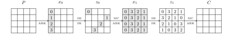
Two Chosen Plaintexts. If the adversary is given twochosen plaintexts, then the time complexity can be reduced. The adversary asks for the encryption of two plaintexts which differ only in four bytes composing one column. The attack relies on Property 4 below, which cleverly uses the linearity in the key-schedule of the AES.

Property 4. For alli¥1 we have the following equations:

i) zi1r4..7s `zir0..3s `zir4..7s M C1

xir4..7s `xi 1r0..3s `xi 1r4..7s

ii) zi1r8..11s `zir4..7s `zir8..11s M C1

xir8..11s `xi 1r4..7s `xi 1r8..11s

iii) zi1r12..15s `zir8..11s `zir12..15s M C1

xir12..15s `xi 1r8..11s `xi 1r12..15s

Proof. Here again the idea is to exploit the interaction between the linearity of MixColumns and the linear operations in the key-schedule. We only prove the first equation (the proofs of the other two is quite similar). Expressingy in terms ofwgives:

zi1r4..7s M C1pwi1r4..7sq

We can relatewi1to xi thanks to theAddRoundKeyoperation:

zi1r4..7s M C1pkir4..7s `xir4..7sq

And there, we can exploit the linearity of the key-schedule:

zi1r4..7s M C1pki 1r0..3s `ki 1r4..7s `xir4..7sq

The sub-keys can then be expressed back in terms ofw andx:

zi1r4..7s M C1pwir0..3s `xi 1r0..3s `wir4..7s `xi 1r4..7s `xir4..7sq

And then, the linearity of MixColumnscan be exploited as well:

zi1r4..7s zir0..3s `zir4..7s `M C1pxir4..7s `xi 1r0..3s `xi 1r4..7sq.

[ \

Fig. 3Two chosen plaintexts attack on two AES rounds. Gray bytes indicate the presence of a difference, and hatched bytes indicate the presence of a known difference. If byteiis known inx0, then the actual

values of all the bytes with the same number can be found.

P ARK 0 1 2 3 x0 SB SR 0 1 2 3 z0 MC ARK 1 1 1 1 2 2 2 2 3 3 3 3 0 0 0 0 x1 SB SR 1 1 1 1 2 2 2 2 3 3 3 3 0 0 0 0 z1 MC ARK C

Assume thatx0r0sis known: it is possible to deduce there from the value (and the difference) inz0r0s,

and finally the difference inx1r0..3s(by Property 2). Because the difference in y1r0..3scan be deduced

from the ciphertexts, it follows that the actual values inx1r0..3s can be deduced thanks to Property 1.

This also reveals bytes 0,7,10 and 13 ofz1 (observe Figure 3). It follows that ifx0r0..3swere known, then

the key could easily be deduced. The attack works by constructing a set of possibles values ofx0r0..3sof

(19)

Algorithm 4Pseudo-code of the attack on 2 rounds using 2 chosen plaintexts.

1: function2R-2CP-Attack(P, C)

2: for allx0r2s PF28 do BuildT2

3: computez0r10sandx1r8..11s

4: letux1r8..11s `Cr4..7s `Cr8..11sin

5: letiz0r10s ` p0d,09,0e,0bq uin

6: T2ris ÐT2ris Y tx0r2su

7: end for

8: for allx0r3s PF28 do BuildT3

9: computez0r7sandx1r4..7s

10: letux1r4..7s `Cr0..3s `Cr4..7sin

11: letiz0r7s ` p0b,0d,09,0eq uin

12: T3ris ÐT3ris Y tx0r3su

13: end for

14: for allx0r1s PF28 do Retrieve the key

15: Computez0r13s, x1r12..15s, z1r3s, z1r6s, z1r9s, z1r12s

16: Computez1r13s Using property 4

17: Computex1r1s, the difference inz0r1s, andx0r0s

18: Computez0r0s, x1r0..3s, z1r0s, z1r7sandz1r10s

19: Readpossible value(s) ofx0r2sinT2

z1r6s `z1r10s 20: Readpossible value(s) ofx0r3sinT3

z1r3s `z1r7s 21: Computek2and check for correctness

22: end for

23: end function

1. We first show that once x0r1sis known, then x0r0s can be determined using Property 4, item iii).

The equation is:

z0r12..15s `z1r8..11s `z1r12..15s M C1

x1r12..15s `Cr8..11s `Cr12..15s ,

We enumerate the possible values of x0r1s and compute all the bytes marked “1” in Figure 3. At

this stage, the right-hand side the equation is fully known. In the left-hand side, z0r13s and z1r9s

are known, and therefore z1r13scan be deduced by projecting the (vector) equation on the second

component. The actual values and the differences can then be deduced in x1r1s, which reveals the

difference in z0r0s (by Property 2). The actual values inx0r0s can then be deduced by Property 1.

We expect on average one possible value of x0r0sper value ofx0r1s.

2. We then seek to extend this procedure to x0r2s and x0r3s. To this end, we still use Property 4,

equationii):

z1r4..7s `z1r8..11s z0r8..11s `M C1

x1r8..11s `Cr4..7s `Cr8..11s , (♣)

The third coordinate of the right-hand side can be entirely deduced from x0r2s. We can therefore

build a table yielding x0r2s from the third coordinate of the right-hand side of p♣q, as shown in

Algorithm 4, lines 2–7.

We perform the same operations withx0r3s, using Property 4, equationi):

z1r0..3s `z1r4..7s z0r4..7s `M C1

x1r4..7s `Cr0..3s `Cr4..7s , (♥)

Here, the fourth coordinate of the right-hand side can be entirely deduced fromx0r3s. We therefore

build a table yielding x0r3s from the third coordinate of the right-hand side ofp♥q (as shown in

Algorithm 4, lines 8–13).

3. Once the two tables T2 and T3 have been built, we are ready to derive x0r2s and x0r3s. For this

purpose, we enumerate the values of x0r1s, derive x0r0s as explained above. The third component

of equation (♣) and the fourth component of (♥) can be computed, and thanks to T2 and T3 the

corresponding values ofx0r2sandx0r3scan be retrieved in constant time, resulting in an average of

256 suggestion for the first column of x0. From there,k2 can be deduced, and the key-schedule can

be inverted to retrieve k0.

5.3 Extensions to Three-Round AES

(20)

Two Chosen Plaintexts. The 2 rounds/2-chosen plaintext attack of section 5.2 can easily be leveraged into a 3-round attack of complexity 216_{, thus improving on a manually-found attack with complexity 2}32

described in [BDD 10].

In this improved attack, the adversary asks for the encryption of two plaintexts which differ only in the first byte. By guessing k0r0s, the adversary obtains the differences inx1r0..3s. This is sufficient

to apply the attack of section 5.2 to rounds 2 and 3. The complexity of the process is therefore 216

encryptions.

Improvement to the Piret-Quisquater Fault Attack. In the Piret-Quisquater fault attack, against the full AES, an unknown difference is introduced in byte 0 of the internal state x7. The adversary

observes the output difference, and recovers the secret key in time 232 _{[PQ03]. We show an improved}

procedure that recovers the key after the equivalent of 224_encryptions.

The attack considers the last three rounds (rounds 8, 9 and 10), but to be consistent with the other three-round attack, we number the attacked rounds 1, 2 and 3. In this setting,the plaintext is unknown, and the only information is that there is a non-zero difference δin x0r0s. For the sake of simplicity, we

describe the attack assuming that the finalMixColumnsoperation hasnot been removed. The attack can be replayed without it, but some details become significantly messier.

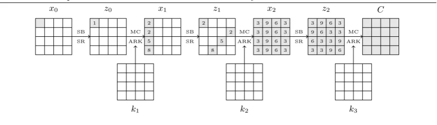
Fig. 4 Fault attack against the AES. Gray square indicates the presence of a difference. The number indicates the step of the attack in which the value of each byte is discovered.

x0

SB

SR 1

z0

MC

ARK 2

2

5

8

x1

SB

SR 2

2

5

8

z1

MC

ARK 3

3

3 9

9

9 6

6

6 3

3

x2

SB

SR

3 9 6 3

z2

MC

ARK

C

k1 k2 k3

One possible way to view this attack would be to guess the “fault” difference δ, to guess the actual value of x0r0s, to derive the difference in x1r0..3s, and to apply the two-round attack of section 5.2

to rounds 2-3. However, it is possible to give a more direct yet pleasantly simple description of the key-recovery.

1. Guess the difference in z0r0s

2. Guess the actual value ofx1r0sandx1r1s

3. Compute the difference inx2r0..3sandx2r12..15s, then the actual values thanks to Property 1.

4. Use Property 4, withi2 andj3 (second component of the vector equation) to filter the guesses. Only 216_{out of 2}24 _{should pass the test.}

5. Guess the actual value ofx1r2s

6. Compute the difference inx2r8..11s, then the actual values.

7. Use Property 4 with i2 andj 2 (third component of the vector equation) to filter the guesses of step 5. Only 216 _{should pass.}

8. Guess the actual value ofx1r3s

9. Compute the difference inx2r4..7s, then the actual values.

10. Use Property 4 withi2 and j1 (fourth component of the vector equation) to filter the guesses of step 8. Only 216 _{should pass.}

11. At this point we should have 216_{candidates for the actual values and the differences in}_x

1r0..3s. From

those, x2 can be reconstructed entirely, as well ask3. It remains to simply test all the candidates.

5.4 Attacks on Four-Round AES