R E S E A R C H
Open Access
Statistical resolution limit for the
multidimensional harmonic retrieval model:
hypothesis test and Cramér-Rao Bound
approaches
Mohammed Nabil El Korso
*, Rémy Boyer, Alexandre Renaux and Sylvie Marcos
Abstract
The statistical resolution limit (SRL), which is defined as the minimal separation between parameters to allow a correct resolvability, is an important statistical tool to quantify the ultimate performance for parametric estimation problems. In this article, we generalize the concept of the SRL to the multidimensional SRL (MSRL) applied to the multidimensional harmonic retrieval model. In this article, we derive the SRL for the so-called multidimensional harmonic retrieval model using a generalization of the previously introduced SRL concepts that we call multidimensional SRL (MSRL). We first derive the MSRL using an hypothesis test approach. This statistical test is shown to be asymptotically an uniformly most powerful test which is thestrongestoptimality statement that one could expect to obtain. Second, we link the proposed asymptotic MSRL based on the hypothesis test approach to a new extension of the SRL based on the Cramér-Rao Bound approach. Thus, a closed-form expression of the asymptotic MSRL is given and analyzed in the framework of the multidimensional harmonic retrieval model. Particularly, it is proved that the optimal MSRL is obtained for equi-powered sources and/or an equi-distributed number of sensors on each multi-way array.
Keywords:Statistical resolution limit, Multidimensional harmonic retrieval, Performance analysis, Hypothesis test, Cramér-Rao bound, Parameter estimation, Multidimensional signal processing
Introduction
The multidimensional harmonic retrieval problem is an important topic which arises in several applications [1]. The main reason is that the multidimensional harmonic retrieval model is able to handle a large class of applica-tions. For instance, the joint angle and carrier estimation in surveillance radar system [2,3], the underwater acous-tic multisource azimuth and elevation direction finding [4], the 3-D harmonic retrieval problem for wireless channel sounding [5,6] or the detection and localization of multiple targets in a MIMO radar system [7,8].
One can find many estimation schemes adapted to the multidimensional harmonic retrieval estimation pro-blem, see, e.g., [1,2,4-7,9,10]. However, to the best of
our knowledge, no work has been done on the resolva-bility of such a multidimensional model.
The resolvability of closely spaced signals, in terms of parameter of interest, for a given scenario (e.g., for a given signal-to-noise ratio (SNR), for a given number of snapshots and/or for a given number of sensors) is a former and challenging problem which was recently updated by Smith [11], Shahram and Milanfar [12], Liu and Nehorai [13], and Amar and Weiss [14]. More pre-cisely, the concept of statistical resolution limit (SRL), i. e., the minimum distance between two closely spaced signalsaembedded in an additive noise that allows a cor-rect resolvability/parameter estimation, is rising in sev-eral applications (especially in problems such as radar, sonar, and spectral analysis [15].)
The concept of the SRL was defined/used in several manners [11-14,16-24], which could turn in it to a con-fusing concept. There exist essentially three approaches * Correspondence: [email protected]
Laboratoire des Signaux et Systèmes (L2S), Université Paris-Sud XI (UPS), CNRS, SUPELEC, 3 Rue Joliot Curie, Gif-Sur-Yvette 91192, France
to define/obtain the SRL. (i) The first is based on the concept of mean null spectrum: assuming, e.g., that two signals are parameterized by the frequencies f1 and f2, the Cox criterion [16] states that these sources are resolved, w.r.t. a given high-resolution estimation algo-rithm,if the mean null spectrum at each frequency f1
and f2 is lower than the mean of the null spectrum at
the midpoint f1+f2
2 . Another commonly used criterion, also based on the concept of the mean null spectrum, is the Sharman and Durrani criterion [17], which states that two sources are resolvedif the second derivative of
the mean of the null spectrum at the midpoint f1+f2
2 is
negative. It is clear that the SRL based on the mean null spectrum is relevant to a specific high-resolution algo-rithm (for some applications of these criteria one can see [16-19] and references therein.) (ii) The second approach is based on detection theory: the main idea is to use a hypothesis test to decide if one or two closely spaced signals are present in the set of the observations. Then, the challenge herein is to link the minimum separation, between two sources (e.g., in terms of fre-quencies) that is detectable at a given SNR, to the prob-ability of false alarm, Pfaand/or to the probability of detectionPd. In this spirit, Sharman and Milanfar [12] have considered the problem of distinguishing whether the observed signal contains one or two frequencies at a given SNR using the generalized likelihood ratio test (GLRT). The authors have derived the SRL expressions w.r.t.Pfa andPdin the case of real received signals, and unequal and unknown amplitudes and phases. In [13], Liu and Nehorai have defined a statistical angular reso-lution limit using the asymptotic equivalence (in terms of number of observations) of the GLRT. The challenge was to determine the minimum angular separation, in the case of complex received signals, which allows to resolve two sources knowing the direction of arrivals (DOAs) of one of them for a given Pfa and a given Pd. Recently, Amar and Weiss [14] have proposed to deter-mine the SRL of complex sinusoids with nearby fre-quencies using the Bayesian approach for a given correct decision probability. (iii) The third approach is based on a estimation accuracy criteria independent of the estimation algorithm. Since the Cramér-Rao Bound (CRB) expresses a lower bound on the covariance matrix of any unbiased estimator, then it expresses also the ultimate estimation accuracy [25,26]. Consequently, it could be used to describe/obtain the SRL. In this con-text, one distinguishes two main criteria for the SRL based on the CRB: (1) the first one was introduced by Lee [20] and states that:two signals are said to be resol-vable w.r.t. the frequencies if the maximum standard deviation is less than twice the difference between f1 and
f2. Assuming that the CRB is a tight bound (under mild/ weak conditions), the standard deviation,σˆf1andσfˆ2, of
an unbiased estimator ˆf= [f1ˆ ˆf2]Tis given byCRB(f1) and CRB(f2), respectively. Consequently, the SRL is defined, in the Lee criterion sense, as 2max
CRB(f1),
CRB(f2)
. One can find some results and applications in [20,21] where this criterion is used to derive a matrix-based expression (i.e., without analytic inversion of the Fisher information matrix) of the SRL for the frequency estimates in the case of the condi-tional and uncondicondi-tional signal source models. On the other hand, Dilaveroglu [22] has derived a closed-form expression of the frequency resolution for the real and complex conditional signal source models. However, one can note that the coupling between the parameters, CRB(f1,f2) (i.e., the CRB for the cross parametersf1and
f2), is ignored by this latter criterion. (2) To extend this, Smith [11] has proposed the following criterion:two sig-nals are resolvable w.r.t. the frequencies if the difference between the frequencies,δf, is greater than the standard
deviation of the DOA difference estimation. Since, the
standard deviation can be approximated by the CRB, then, the SRL, in the Smith criterion sense, is defined as the limit of δf for which δf <
CRB(δf)is achieved. This means that, the SRL is obtained by solving the fol-lowing implicit equation
δ2
f = CRB(δf) = CRB(f1) + CRB(f2)−2CRB(f1,f2).
In [11,23], Smith has derived the SRL for two closely spaced sources in terms of DOA, each one modeled by one complex pole. In [24], Delmas and Abeida have derived the SRL based on the Smith criterion for DOA of discrete sources under QPSK, BPSK, and MSK model assumptions. More recently, Kusuma and Goyal [27] have derived the SRL based on the Smith criterion in sampling estimation problems involving a powersum series.
It is important to note that all the criteria listed before take into account only one parameter of interest per sig-nal. Consequently, all the criteria listed before cannot be applied to the aforementioned the multidimensional harmonic model. To the best of our knowledge, no results are available on the SRL for multiple parameters of interest per signal. The goal of this article is to fill this lack by proposing and deriving the so-called MSRL for the multidimensional harmonic retrieval model.
link the asymptotic MSRL based on the hypothesis test approach to a new extension of the MSRL based on the CRB approach. Furthermore, we show that the MSRL based on the CRB approach is equivalent to the MSRL based on the hypothesis test approach for a fixed couple (Pfa, Pd), and (iii) the hypothesis test is shown to be asymptotically an uniformly most powerful test which is
the strongest statement of optimality that one could
expect to obtain [28].
The article is organized as follows. We first begin by introducing the multidimensional harmonic model, in section “Model setup”. Then, based on this model, we obtain the MSRL based on the hypothesis test and on the CRB approach. The link between theses two MSRLs is also described in section“Determination of the MSRL for two sources” followed by the derivation of the MSRL closed-form expression, where, as a by product the exact closed-form expressions of the CRB for the multi-dimensional retrieval model is derived (note that to the best of our knowledge, no exact closed-form expressions of the CRB for such model is available in the literature). Furthermore, theoretical and numerical analyses are given in the same section. Finally, conclusions are given.
Glossary of notation
The following notations are used through the article. Column vectors, matrices, and multi-way arrays are represented by lower-case bold letters (a, ...), upper-case bold letters (A, ...) and bold calligraphic letters(A, ...), whereas
• ℝ and ℂ denote the body of real and complex values, respectively,
•RD1×D2×···×DIandCD1×D2×···×DIdenote the real and
complex multi-way arrays (also called tensors) body of dimension D1 ×D2× ... ×DI, respectively,
•j= the complex number√−1.
•IQ= the identity matrix of dimensionQ,
•0Q1×Q2= theQ1×Q2 matrix filled by zeros,
•[a]i= theith element of the vector a,
•[A]i1,i2= thei1th row and thei2th column element
of the matrixA,
•[A]i1,i2,...,iN= the (i1,i2, ...,iN)th entry of the
multi-way arrayA,
•[A]i,p:q = the row vector containing the (q -p+ 1)
elements [A]i,k, wherek=p, ...,q,
•[A]p:q,k= the column vector containing the (q-p+
1) elements [A]i,k, wherei=p, ...,q,
• the derivative of vector a w.r.t. to vector b is
defined as follows:
∂
a ∂b
i,j = ∂[a]i
∂[b]j,
•AT
= the transpose of the matrix A,
•A* = the complex conjugate of the matrixA,
•AH
= (A*)T,
•tr {A} = the trace of the matrixA,
•det {A} = the determinant of the matrixA,
•ℜ{a} = the real part of the complex numbera,
•E{a}= the expectation of the random variablea,
•||a||2= 1 L
L
t=1[a]2t denotes the normalized norm of the vectora(in whichLis the size ofa),
•sgn (a) = 1 ifa≥0 and -1 otherwise.
• diag(a) is the diagonal operator which forms a diagonal matrix containing the vector a on its diagonal,
•vec(.) is the vec-operator stacking the columns of a matrix on top of each other,
•⊙stands for the Hadamard product,
•⊗stands for the Kronecker product,
• ○ denotes the multi-way array outer-product
(recall that for a given multi-way arrays
A∈CA1×A2×···×AI andB∈CB1×B2×···×BJ, the result of
the outer-product of A and B denoted by
CA1×···×AI×B1×···×BJ is given by
[C]a1,...,aI,b1,...,bJ= [A◦B]a1,...,aI,b1,...,bJ = [A]a1,...,aI[B]b1,...,bJ).
Model setup
In this section, we introduce the multidimensional har-monic retrieval model in the multi-way array form (also known astensor form[29]). Then, we use the PARAFAC (PARallel FACtor) decomposition to obtain a vector form of the observation model. This vector form will be used to derive the closed-form expression of the MSRL.
Let us consider a multidimensional harmonic model consisting of the superposition of two harmonics each one of dimensionP contaminated by an additive noise. Thus, the observation model is given as follows [8,9,26,30-32]:
[Y(t)]n1,...,nP= [X(t)]n1,...,nP+[N(t)]n1,...,nP, t= 1,. . .,L, and np= 0,. . .,Np−1,ð1Þ
whereY(t),X(t), andN(t)denote the noisy observa-tion, the noiseless observaobserva-tion, and the noise multi-way array at thetth snapshot, respectively. The number of snapshots and the number of sensors on each array are denoted byLand (N1, ...,NP), respectively. The noiseless
observation multi-way array can be written as followsb [26,30-32]:
[X(t)]n1,...,nP =
2
m=1 sm(t)
P
p=1
ejωm(p)np, (2)
where ω(p)
mandsm(t) denote the mth frequency viewed
jm(t) denote the real positive amplitude and the phase for the mth signal source at the tth snapshot, respectively.
Since,
P
p=1
ejω(p)mnp =
a(ω(1)m )◦a(ωm(2))◦ · · · ◦a(ω(mP))
n1,n2,...,nP ,
wherea(.) is a Vandermonde vector defined as
a(ω(mp)) =
1 ejω(p)m · · · ej(N
p−1)ω(mp)
T
,
then, the multi-way arrayX(t)follows a PARAFAC decomposition [7,33]. Consequently, the noiseless obser-vation multi-way array can be rewritten as follows:
X(t) =
2
m=1 sm(t)
a(ωm(1))◦a(ωm(2))◦ · · · ◦a(ωm(P))
. (3)
First, let us vectorize the noiseless observation as follows:
vec(X(t)) =[X(t)]0,0,...,0· · ·[X(t)]N1−1,0,···,0[X(t)]0,1,...,0· · ·[X(t)]N1−1,N2−1,...,NP−1 T
.ð4Þ
Thus, the full noise-free observation vector is given by
x=vecT(X(1)) vecT(X(2))· · ·vecT(X(L))T.
Second, and in the same way, we definey, the noisy observation vector, andn, the noise vector, by the con-catenation of the proper multi-way array’s entries, i.e.,
y=vecT(Y(1)) vecT(Y(2))· · ·vecT(Y(L))T=x+n. (5)
Consequently, in the following, we will consider the observation model in (5). Furthermore, the unknown parameter vector is given by
ξ =ωTρTT, (6)
where ωdenotes the unknown parameter vector of interest, i.e., containing all the unknown frequencies
ω=
(ω(1))T· · ·(ω(P))T
T
,
in which
ω(p)=ω(p)
1 ω
(p) 2
T
. (7)
whereas rcontains the unknown nuisance/unwanted parameters vector, i.e., characterizing the noise covar-iance matrix and/or amplitude and phase of each source (e.g., in the case of a covariance noise matrix equal to
σ2I
LN1...NP and unknown deterministic amplitudes and
phases, the unknown nuisance/unwanted parameters vectorris given byr= [a1(1) ...a2(L)j1(1) ...j2(L)s2]T.
In the following, we conduct a hypothesis test formu-lation on the observation model (5) to derive our MSRL expression in the case of two sources.
Determination of the MSRL for two sources
Hypothesis test formulation
Resolving two closely spaced sources, with respect to their parameters of interest, can be formulated as a bin-ary hypothesis test [12-14] (for the special case of P= 1). To determine the MSRL (i.e.,P ≥1), let us consider the hypothesisH0which represents the case where the two emitted signal sources are combined into one signal, i.e., the two sources have the same parameters (this hypothesis is described by ∀p∈[1. . .P],ω1(p)=ω(2p)), whereas the hypothesisH1embodies the situation where the two signals are resolvable (the latter hypothesis is described by∃pÎ[1 ... P], such thatω1(p)=ω(2p)). Conse-quently, one can formulate the hypothesis test, as a sim-ple one-sided binary hypothesis test as follows:
H
0:δ= 0,
H1:δ >0, (8)
where the parameter δis the so-called MSRL which indicates us in which hypothesis our observation model belongs. Thus, the question addressed below is how can we define the MSRLδsuch that all thePparameters of interest are taken into account? A natural idea is thatδ reflects a distance between theP parameters of interest. Let the MSRL denotes the l1 normcbetween two sets containing the parameters of interest of each source (which is the naturally used norm, since in the mono-parameter frequency case that we extend here, the SRL is defined asδ =f1 - f2 [13,14,34]). Meaning that, if we
denote these sets as C1 and C2 where
Cm=
ω(1)
m ,ω(2)m ,. . .,ω(mP)
, m = 1,2, thus, δ can be
defined as
δ P
p=1
ω(p)
2 −ω
(p)
1 . (9)
First, note that the proposed MSRL describes well the hypothesis test (8) (i.e., δ = 0 means that the two emitted signal sources are combined into one signal and δ≠0 the two signals are resolvable). Second, since the MSRLδis unknown, it is impossible to design an opti-mal detector in the Neyman-Pearson sense. Alterna-tively, the GLRT [28,35] is a well-known approach appropriate to solve such a problem. To conduct the GLRT on (8), one has to express the probability density function (pdf) of (5) w.r.t.δ. Assuming (without loss of generality) that ω(1)1 > ω2(1), one can notice that ξ is
known if and only ifδandϑω(1)2 (ω(2))T. . .(ω(P))T
are fixed (i.e., there is a one to one mapping betweenδ,
ϑ, andξ). Consequently, the pdf of (5) can be described asp(y|δ,ϑ). Now, we are ready to conduct the GLRT for this problem:
LG(y) =
maxδ,ϑ1p(y|δ,ϑ1,H1)
maxϑ0p(y|ϑ0,H0)
= p(y|ˆδ,ϑˆ1,H1)
p(y| ˆϑ0,H0) H1
≷
H0 ς,
(10)
where δˆ,ϑˆ1, andϑˆ0denote the maximum likelihood estimates (MLE) ofδunderH1, the MLE ofϑ underH1 and the MLE of ϑunderH0, respectively, and where ς’ denotes the test threshold. From (10), one obtains
TG(y) = LnLG(y)
H1 ≶
H0
ς= Lnς, (11)
in which Ln denotes the natural logarithm.
Asymptotic equivalence of the MSRL
Finding the analytical expression of TG(y) in (11) is not
tractable. This is mainly due to the fact that the deriva-tion ofδˆis impossible since from (2) one obtains a mul-timodal likelihood function [36]. Consequently, in the following, and as ind[13], we consider the asymptotic case (in terms of the number of snapshots). In [35, eq (6C.1)], it has been proven that, for a large number of snapshots, the statistic TG(y) follows a chi-square pdf
underH0and H1given by
TG(y)∼
χ2
1 underH0,
χ2
1(κ(Pfa,Pd)) underH1, (12) whereχ2
1 andχ21(κ(Pfa,Pd))denote the central chi-square and the noncentral chi-chi-square pdf with one degree of freedom, respectively.Pfaand Pd are, respec-tively, the probability of false alarm and the probability of detection of the test (8). In the following, CRB(δ) denotes the CRB for the parameter δ where the unknown vector parameter is given by [δϑT]T. Conse-quently, assuming that CRB(δ) exists (under H0and
H1), is well defined (see section “MSRL closed-form expression” for the necessaryeand sufficient conditions) and is a tight bound (i.e., achievable under quite gen-eral/weak conditions [36,37]), thus the noncentral para-meter’(Pfa,Pd) is given by [[35], p. 239]
κ(Pfa,Pd) =δ2(CRB(δ))−1. (13)
On the other hand, one can notice that the noncentral parameter ’(Pfa, Pd) can be determined numerically by the choice ofPfaandPd[13,28] as the solution of
Q−1 χ2
1(Pfa) =Q
−1 χ2
1(κ(Pfa,Pd))(Pd), (14)
in whichQ−χ21
1()andQ
−1 χ2
1(κ(Pfa,Pd))()are the inverse
of the right tail of theχ12andχ21(κ(Pfa,Pd))pdf start-ing at the value ϖ. Finally, from (13) and (14) one obtainsf
δ=κ(Pfa, Pd)CRB(δ), (15)
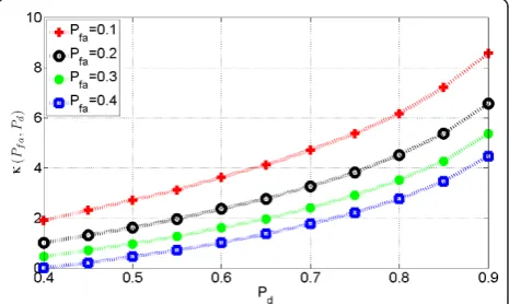
whereκ(Pfa,Pd) =κ(Pfa,Pd)is the so-called transla-tion factor [13] which is determined for a given prob-ability of false alarm and probprob-ability of detection (see Figure 1 for the behavior of the translation factor versus
Pfaand Pd).
Result 1:The asymptotic MSRL for model (5) in the
case of P parameters of interest per signal (P ≥ 1) is given byδwhich is the solution of the following equa-tion:
δ2−κ2(Pfa,Pd)(Adirect+Across) = 0, (16)
where Adirect denotes the contribution of the para-meters of interest belonging to the same dimension as follows
Adirect=
P
p=1
CRB(ω(1p)) + CRB(ω (p)
2 )−2CRB(ω (p) 1 ,ω
(p) 2 ),
and whereAcrossis the contribution of the cross terms between distinct dimension given by
Across= P
p=1 P
p=1 p=p
gpgp(CRB(ω(p)1 ,ω1(p)) + CRB(ω2(p),ω(p)
2 )−2CRB(ω (p) 1 ,ω
(p) 2 )),
in which gp= sgn
ω(p)
1 −ω
(p) 2
.
Proofsee Appendix 1.
Remark 1: It is worth noting that the hypothesis test
(8) is a binary one-sided test and that the MLE used is
an unconstrained estimator. Thus, one can deduce that the GLRT, used to derive the asymptotic MSRL [13,35]: (i) is the asymptotically uniformly most powerful test among all invariant statistical tests, and (ii) has an asymptotic constant false-alarm rate (CFAR). Which is, in the asymptotic case, considered as thestrongest state-ment of optimality that one could expect to obtain [28].
•Existence of the MSRL: It is natural to assume that the CRB is a non-increasing (i.e., decreasing or con-stant) function on ℝ+ w.r.t.δsince it is more diffi-cult to estimate two closely spaced signals than two largely-spaced ones. In the same time the left hand side of (15) is a monotonically increasing function w. r.t. δ on ℝ+. Thus for a fixed couple (Pfa, Pd), the solution of the implicit equation given by (15) always exists. However, theoretically, there is no assurance that the solution of equation (15) is unique.
• Note that, in practical situation, the case where CRB(δ) is not a function ofδ is important since in this case, CRB(δ) is constant w.r.t.δ and thus the solution of (15) exists and is unique (see section
“MSRL closed-form expression”).
In the following section, we study the explicit effect of this so-called translation factor.
The relationship between the MSRL based on the CRB and the hypothesis test approaches
In this section, we link the asymptotic MSRL (derived using the hypothesis test approach, see Result 1) to a new proposed extension of the SRL based on the Smith criterion [11]. First, we recall that the Smith criterion defines the SRL in the case of P = 1 only. Then, we extend this criterion toP≥ 1 (i.e., the case of the multi-dimensional harmonic model). Finally, we link the MSRL based on the hypothesis test approach (see Result 1) to the MSRL based on the CRB approach (i.e., the extended SRL based on the Smith criterion).
The Smith criterion: Since the CRB expresses a lower
bound on the covariance matrix of any unbiased estima-tor, then it expresses also the ultimate estimation accu-racy. In this context, Smith proposed the following criterion for the case of two source signals parameter-ized each one by only one frequency [11]: two signals are resolvable if the difference between their frequency,
δω(1) =ω2(1)−ω1(1),is greater than the standard deviation
of the frequency difference estimation. Since, the stan-dard deviation can be approximated by the CRB, then, the SRL, in the Smith criterion sense, is defined as the limit of δω(1)for whichδω(1) <
CRB(δω(1))is achieved.
This means that, the SRL is the solution of the following implicit equation
δ2
ω(1) = CRB(δω(1)).
The extension of the Smith criterion to the case of P≥
1: Based on the above framework, a straightforward extension of the Smith criterion to the case ofP ≥1 for the multidimensional harmonic model is as follows:two multidimensional harmonic retrieval signals are
resolva-ble if the distance between C1 and C2, is greater than
the standard deviation of the δCRB estimation.
Conse-quently, assuming that the CRB exists and is well defined, the MSRL δCRB is given as the solution of the following implicit equation
δ2
CRB= CRB(δCRB)
s.t. δCRB=Pp=1|ω (p)
2 −ω
(P) 1 |.
(17)
Comparison and link between the MSRL based on the CRB approach and the MSRL based on the hypothesis
test approach: The MSRL based on the hypothesis test
approach is given as the solution of
δ=κ(Pfa,Pd)
CRB(δ), s.t. δ=Pp=1ω2(p)−ω(1p),
whereas the MSRL based on the CRB approach is given as the solution of (17). Consequently, one has the following result:
Result 2:Upon to a translation factor, the asymptotic
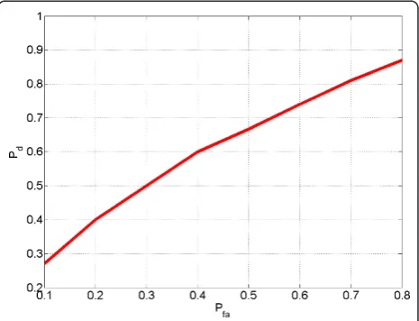
MSRL based on the hypothesis test approach (i.e., using the binary one-sided hypothesis test given in (8)) is equiva-lent to the proposed MSRL based on the CRB approach (i. e., using the extension of the Smith criterion). Conse-quently, the criterion given in (17) is equivalent to an asymptotically uniformly most powerful test among all invariant statistical tests for(Pfa,Pd) = 1 (see Figure 2 for the values of (Pfa,Pd) such that(Pfa,Pd) = 1).
The following section is dedicated to the analytical computation of closed-form expression of the MSRL. In section “Assumptions,” we introduce the assumptions used to compute the MSRL in the case of a Gaussian random noise and orthogonal waveforms. Then, we derive non matrix closed-form expressions of the CRB (note that to the best of our knowledge, no closed-form expressions of the CRB for such model is available in the literature). In “MSRL derivation” and thanks to these expressions, the MSRL wil be deduced using (16). Finally, the MSRL analysis is given.
MSRL closed-form expression
in section“Determination of the MSRL for two sources” we have defined the general model of the multidimen-sional harmonic model. To derive a closed-form expres-sion of the MSRL, we need more assumptions on the covariance noise matrix and/or on the signal sources.
Assumptions
• The noise is assumed to be a complex circular white Gaussian random process i.i.d. with zero-mean and unknown varianceσ2I
LN1...NP.
• We consider a multidimensional harmonic model due to the superposition of two harmonics each of them of dimension P ≥ 1. Furthermore, for sake of simplicity and clarity, the sources have been assumed known and orthogonal (e.g., [7,38]). In this case, the unknown parameter vector is fixed and does not grow with the number of snapshots. Consequently, the CRB is an achievable bound [36].
•Each parameter of interest w.r.t. to the first signal,
ω(p)
1 p= 1. . .P, can be as close as possible to the parameter of interest w.r.t. to the second signal
ω(p)
2 p= 1. . .P, but not equal. This is not really a restrictive assumption, since in most applications, having two or more identical parameters of interest is a zero probability event [[9], p. 53].
Under these assumptions, the joint probability density function of the noisy observations y for a given unknown deterministic parameter vectorξis as follows:
p(y|ξ) = L
t=1
p(vec(Y(t))|ξ) = 1 (πσ2)LNe
−1
σ2 (y−x) H
(y−x)
,
where N=Pp=1Np. The multidimensional harmonic retrieval model with known sources is considered herein, and thus, the parameter vector is given by
ξ =ωTσ2T, (18)
where
ω=(ω(1))T· · ·(ω(P))TT,
in which
ω(p)=ω(p) 1 ω
(p) 2
T
. (19)
CRB for the multidimensional harmonic model with orthogonal known signal sources
The Fisher information matrix (FIM) of the noisy obser-vationsyw.r.t. a parameter vectorξis given by [39]
FIM(ξ) =E
∂lnp(y|ξ) ∂ξ
∂
lnp(y|ξ) ∂ξ
H
.
For a complex circular Gaussian observation model, the (ith,kth) element of the FIM for the parameter vec-torξis given by [34]
[FIM(ξ)]i,k=LN
σ4
∂σ2
∂[ξ]i
∂σ2
∂[ξ]k
+ 2 σ2
∂
xH
∂[ξ]i
∂x
∂[ξ]k
(i,k) ={1,. . ., 2P+ 1}2.ð20Þ
Consequently, one can state the following lemma.
Lemma 1: The FIM for the sum of two P-order
har-monic models with orthogonal known sources, has a block diagonal structure and is given by
FIM(ξ) = 2 σ2
Fω 02P×1 01×2P ×
, (21)
where, the (2P) × (2P) matrixFωis also a block diago-nal matrix given by
Fω=LN(⊗G), (22)
in whichΔ= diag {||a1||2,||a2||2} where
αm=
αm(1) ... αm(L)
T
for m∈ {1, 2}, (23)
and
[G]k,l=
⎧ ⎪ ⎨ ⎪ ⎩
(2Nk−1)(Nk−1)
6 for k=l,
(Nk−1)(Nl−1)
2 for k=l.
Proofsee Appendix 2.
After some calculation and using Lemma 1, one can state the following result.
Result 3:The closed-form expressions of the CRB for
the sum of twoP-order harmonic models with orthogo-nal known sigorthogo-nal sources are given by
CRB(ω(mp)) = 6
LNSNRm
whereSNRm= ||αm|| 2
σ2 denotes the SNR of the mth source and where
Cp=
Np(1−3VP) + 3VP+ 1
(Np+ 1)(Np2−1)
in which VP=
1
1 + 3Pp=1 Np−1 Np+1
.
Furthermore, the cross-terms are given by
CRB(ω(mp),ω(p
)
m ) = ⎧ ⎨ ⎩
0 form=m,
−6 LNSNRm
˜
Cp,pform=mandp=p, (25)
where
˜
Cp,p= 3VP
(Np+ 1)(Np+ 1) .
Proofsee Appendix 3.
MSRL derivation
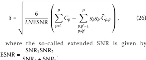
Using the previous result, one obtains the unique solu-tion of (16), thus, the MSRL for model (1) is given by the following result:
Result 4:The MSRL for the sum ofP-order harmonic
models with orthogonal known signal sources, is given by
δ=
6
LNESNR
⎛ ⎜ ⎜ ⎝
P
p=1 Cp−
P
p,p=1 p=p
gpgpC˜p,p
⎞ ⎟ ⎟
⎠, (26)
where the so-called extended SNR is given by
ESNR = SNR1SNR2 SNR1+ SNR2
.
Proofsee Appendix 4.
Numerical analysis
Taking advantage of the latter result, one can analyze the MSRL given by (26):
• First, from Figure 3 note that the numerical solu-tion of the MSRL based on (12) is in good agree-ment with the analytical expression of the MSRL (23), which validate the closed-form expression given in (23). On the other hand, one can notice that, for
Pd= 0.37 andPfa= 0.1 the MSRL based on the CRB is exactly equal to the MSRL based on hypothesis test approach derived in the asymptotic case. From the case Pd = 0.49 and Pfa= 0.3 or/and Pd = 0.32 and Pfa= 0.1, one can notice the influence of the translation factor (Pfa,Pd) on the MSRL.
•The MSRLgisO(
%
1
ESNR)which is consistent with some previous results for the case P = 1 (e.g., [12,14,24]).
•From (26) and for a large number of sensorsN1=
N2 = ... =NP=N≫1, one obtains a simple
expres-sion
δ=
%
12
LNP+1ESNR P
1 + 3P,
meaning that, the SRL isO(
%
1
NP+1).
•Furthermore, since P ≥1, one has
(P+ 1) (3P+ 1)
P(3P+ 4) <1,
and consequently, the ratio between the MSRL of a multidimensional harmonic retrieval withP parameters of interest, denoted byδPand the MSRL of a
multidi-mensional harmonic retrieval with P+ 1 parameters of interest, denoted byδP+1, is given by
δP+1
δP =
&
(P+ 1)(3P+ 1)
NP(3P+ 4) , (27)
meaning that the MSRL forP+ 1 parameters of inter-est is less than the one for Pparameters of interest (see Figure 4). This, can be explained by the estimation addi-tional parameter and also by an increase of the received noisy data thanks to the additional dimension. One should note that this property is proved theoretically thanks to (27) using the assumption of an equal and large number of sensors. However, from Figure 4 we notice that, in practice, this can be verified even for a
small number of sensors (e.g., in Figure 4 one has 3 ≤
Np≤5 forp= 3, ..., 6).
•Furthermore, since
%
4
LNP+1ESNR ≤δP< δP−1<· · ·< δ1
one can note that, the SRL is lower bounded by
%
4
LNP+1ESNR.
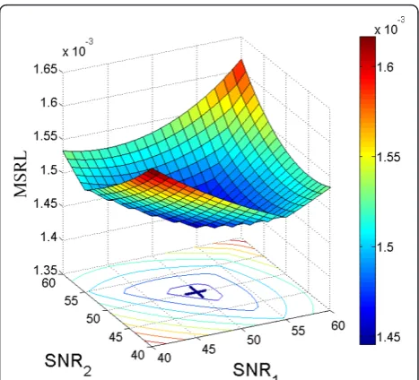
• One can address the problem of finding the opti-mal distribution of power sources making the SRL the smallest as possible (s.t. the constraint of con-stant total source power). In this issue, one can state the following corollary: Corollary 1: The optimal power’s source distribution that ensures the smallest MSRL is obtained only for the equi-powered sources case.
Proofsee Appendix 5.
This result was observed numerically forP = 1 in [12] (see Figure 5 for the multidimensional harmonic model). Moreover, it has been shown also by simulation for the caseP= 1 that the so-called maximum likelihood break-down (i.e., when the mean square error of the MLE increases rapidly) occurs at higher SNR in the case of different power signal sources than in the case of equi-powered signal sources [40]. The authors explained it by the fact that one source grabs most of the total power, then, this latter will be estimated more accurately, whereas the second one, will take an arbitrary parameter
estimation which represents an outlier.
•In the same way, let us consider the problem of the optimal placement of the sensorsh N1, ...,NP , making the minimum MSRL s.t. the constraint that the total number of sensors is constant (i.e., Ntotal=Pp=1Npin which we suppose thatNtotal is a multiple ofP).
Corollary 2:If the total number of sensorsNtotal, is a multiple of P, then an optimal placement of the sensors that ensure the lowest MSRL is (see Figure 6 and 7)
N1=· · ·=NP= Ntotal
P . (28)
Proofsee Appendix 6.
Remark 3:Note that, in the case whereNtotalis not a multiple of P, one expects that the optimal MSRL is given in the case where the sensors distribution approaches the equi-sensors distribution situation given in corollary 3. Figure 7 confirms that (in the case ofP= 3,N1 = 8 and a total number of sensorsN= 22). From Figure 7, one can notice that the optimal distribution of the number of sensors corresponds toN2 =N3 = 7 and
N1= 8 which is the nearest situation to the equi-sensors distribution.
Figure 5 MSRL versus SNR1, the SNR of the first source, and
SNR2, the SNR of the second source. One can notice that the optimal distribution of the SNR (which corresponds to the lowest
MSLR) corresponds toSNR1= SNR2= SNRtotal
2 as predicted by Corollary 1.
Conclusion
In this article, we have derived the MSRL for the multi-dimensional harmonic retrieval model. Toward this end, we have extended the concept of SRL to multiple para-meters of interest per signal. First, we have used a hypothesis test approach. The applied test is shown to be asymptotically an uniformly most powerful test which is thestrongest statement of optimality that one could hope to obtain. Second, we have linked the asymptotic MSRL based on the hypothesis test approach to a new extension of the SRL based on the Cramér-Rao bound approach. Using the Cramér-Rao bound and a
proper change of variable formula, closed-form expres-sion of the MSRL are given.
Finally, note that the concept of the MSRL can be used to optimize, for example, the waveform and/or the array geometry for a specific problem.
Appendix 1
The proof of Result 1
Appendix 1.1: In this appendix, we derive the MSRL
using thel1norm.
From CRB(ξ) where ξ = [ωT rT]T in which ω= [ω(1)1 ω(1)2 ω1(2)ω2(2)· · ·ω(1P)ω2(P)]T, one can deduce CRB(ξ) where ξ=g(ξ) = [δϑT]T in which ϑ[ω2(1)(ω(2))T· · ·(ω(P))T]T. Thanks to the Jacobian matrix given by
∂g(ξ) ∂ξ =
⎡
⎣h
T0
A 0 0 I
⎤
⎦,
where h = [g1g2 ... gP ]T ⊗ [1 - 1]T, in which
gp= ∂δ
∂ω(p) 1
=− ∂δ ∂ω(p)
2
= sgn (ω(1p)−ω2(p))and A = [0 I].
Using the change of variable formula
CRB(ξ) = ∂g( ξ) ∂ξ
CRB(ξ)
⎛
⎝∂g(
ξ) ∂ξ
⎞ ⎠
T
, (29)
one has
CRB(ξ) =
hTCRB(ω)h×
× I
.
Consequently, after some calculus, one obtains
CRB(δ)[CRB(ξ)]1,1=hTCRB(ω)h
=
2P
p=1 2P
p=1
[h]p[h]p[CRB(ω)]p,p
=
P
p=1 P
p=1
gpgp
[CRB(ξ)]2p,2p+ [CRB(ξ)]2p−1,2p−1−[CRB(ξ)]2p,2p−1−[CRB(ξ)]2p−1,2p
Adirect+Across,
ð30Þ
where
Adirect=Pp=1CRB(ω1(p)) + CRB(ω2(p))−2CRB(ω1(p),ω2(p)) and where Across(k) =
P
p=1
P
p=1 p=p
gpgp
CRB(ω(p) 1,ω
(p) 1 ) + CRB(ω
(p) 2,ω
(p) 2 )−2CRB(ω
(p) 1,ω
(p) 2 )
Finally using (30) one obtains (16)
Appendix 1.2:In this part, we derive the MSRL using
the lk norm for a given integer k ≥1. The aim of this part is to support the endnote a, which stays that using thel1norm computing the MSRL using the l1 norm is for the calculation convenience.
Once again, from CRB(ξ), one can deduceCRB(ξk) where ξk=gk(ξ) = [δ(k)ϑT]T in which the distance betweenC1 andC2using thelknorm is given byδ(k)≜
Figure 7The plot of the MSRL versusN2in the case ofP= 3,
N1= 8 and a total number of sensorsN= 22.
Figure 6The MSRL versusN1andN2in the case ofP= 3 and a
total number of sensorsNtotal= 21. One can notice that the optimal distribution of the number of sensors (which corresponds
k-norm distance(C1,C2) =
P
p=1δpk
1/k
and where
ϑ[ω(1)2 (ω(2))T. . .(ω(P))T]T. The Jacobian matrix is given by
∂g(ξ) ∂ξ = ⎡ ⎣h T k0 A 0 0 I ⎤ ⎦,
wherehk = [1 - 1]T ⊗[g1(k)g2(k) ... gP(k)]T, in which
gp(k) = ∂δ (k) ∂ω(p) 1
=−∂δ(k) ∂ω(p) 2
andA= [0I]. Since |x|kcan be
written as√x2k. Thus, for × ≠0, one has
gp(k) = ∂
+
P
p=1 %
ω(p) 1 −ω
(p) 2
2k,1/k
∂ω(p) 1
=1 k
+p
i=1 %
ω(i) 1 −ω
(i) 2
2k,
1 k−1∂
% ω(i)
1−ω (i) 2
2k
∂ω(i) 1
= sgn(ω(p) 1 −ω
(p) 2)
⎛ ⎝P
p=1 %
ω(p) 1 −ω
(p) 2
2k ⎞ ⎠ 1 k−1%
ω(p) 1 −ω
(p) 2
2(k−1)
= sgn(ω(p) 1 −ω
(p) 2)δ1−kδkp−1.
ð31Þ
Again, using the change of variable formula (29), one has
CRB(ξk) =
hTkCRB(ω)hk×
× I
.
Consequently, after some calculus, one obtains
CRB(δ(k))[CRB(ξk)]1,1
= P p=1 P
p=1
gp(k)gp(k)([CRB(ξ)]2p,2p+ [CRB(ξ)]2p−1,2p−1−[CRB(ξ)]2p,2p−1−[CRB(ξ)]2p−1,2p) = (δ(k))2(1−k)(A
direct(k) +Across(k)),
ð32Þ
where
Adirect(k) =Pp=1δ 2(k−1) p
CRB(ω(1p)) + CRB(ω(2p))−2CRB(ω(1p),ω(2p))
and where
Across(k) =P
p=1 P
p=1
p=p
δk−1
p δpk−1sgn(ω1(p)−ω(2p))sgn(ω(p ) 1−ω(p
) 2)
CRB(ω(p)
1,ω(p ) 1) + CRB(ω(2p),ω(p
)
2)−2CRB(ω1(p),ω(p ) 2)
. Consequently, note that resolving analytically the implicit equation (32) w.r.t. δ(k) is intractable (aside from some special cases). Whereas, resolving analytically the implicit equation (30) can be tedious but feasible (see section“MSRL closed form expression”).
Furthermore, denotinggp(1) =gp,Across(1)≜Acrossand
Adirect(1)≜Adirectand using (32) one obtains (16).
Appendix 2
Proof of Lemma 1
From (20) one can note the well-known property that the model signal parameters are decoupled from the noise variance [42]. Consequently, the block-diagonal structure in (21) is self-evident.
Now, let us prove (22). From (4), one obtains
∂vec(X(t)) ∂ω(p)
m
=jsm(t)
a(ω(1) m)⊗a(ω
(2)
m)⊗ · · · ⊗a’(ω (p)
m)⊗ · · · ⊗a(ω (P) m)
,
where
a’(ω(mp)) =
0 ejω(mp) . . . (Np−1)ej(Np−1)ω(mp)
T
.
Thus,
∂x
∂ω(p) m
=jsm⊗
a(ω(1)
m )⊗a(ω(2)m )⊗ · · · ⊗a’(ωm(p))⊗ · · · ⊗a(ωm(P))
,
wheresm= [sm(1) ...sm(L)]T. Using the distributivity of
the Hermitian operator over the Kronecker product and the mixed-product property of the Kronecker product [43] and assuming, without loss of generality thatp’<p, one obtains
( ∂x
∂ω(p)
m
)H ∂x ∂ω(p)
m
=sH
m,⊗
aH(ω(1)
m)⊗aH(ω(2)m)⊗ · · · ⊗a’H(ω
(p)
m )⊗ · · · ⊗aH(ω
(P)
m)
×sm⊗
a(ω(1)
m)⊗a(ω(2)m)⊗ · · · ⊗a’(ωm(p))⊗ · · · ⊗a(ω(mP))
= (sH
m,sm)⊗
aH(ω(1)
m)a(ω(1)m)
⊗ · · · ⊗a’H(ω(p)
m)a(ω(mp))
⊗. . .
. . .⊗aH(ω(p)
m )a’(ω(p
)
m)
⊗ · · · ⊗aH(ω(P)
m)a(ω(mP))
.
ð33Þ
On the other hand, one has
aH(ωm(p))a(ωm(p)) =Np, (34)
whereas
aH(ω(p)
m)a’(ω(mp)) =
Np(Np−1)
2 and a’
H(ω(p)
m)a’(ω(mp)) =
Np(2Np−1)(Np−1)
6 ð35Þ
Finally, assuming known orthogonal wavefronts [38] (i. e., sH
m,sm= 0) and replacing (35) and (34) into (33), one obtains + ∂x ∂ω(p) m ,H ∂x ∂ω(p)
m = ⎧ ⎪ ⎪ ⎪ ⎨ ⎪ ⎪ ⎪ ⎩
0 form=m,
L||αm||2N(Np−1)(Np−1)
4 form=m
andp=p,
L||αm||2N(2Np−1)(Np−1)
6 form=m
andp=p,
(36)
where am= [am (1) ...am (L)] form Î{1, 2}:
Conse-quently, using (36),Fωcan be expressed as a block diag-onal matrix
Fω=
J1 0 0 J2
, (37)
where eachP×PblockJmis defined by
Jm=L||αm||2NG, (38)
where G= ⎡ ⎢ ⎢ ⎢ ⎢ ⎢ ⎢ ⎢ ⎢ ⎣
(N1−1)(2N1−1)
6
(N1−1)(N2−1)
4 . . .
(N1−1)(NP−1)
4 (N2−1)(N1−1)
4
(N2−1)(2N2−1)
6 . . .
(N2−1)(NP−1)
4 ..
. ... . .. ...
(NP−1)(N1−1)
4
(N2P−1)(N2−1)
4 · · ·
(NP−1)(2NP−1)
6 ⎤ ⎥ ⎥ ⎥ ⎥ ⎥ ⎥ ⎥ ⎥ ⎦ .
Appendix 3
Proof of Result 3
Using (22) one obtains
CRB(ω) =σ
2
2F
−1
ω = σ
2
2LN(
−1⊗G−1) (39)
where−1= diag
1 ||α1||2
, 1
||α2||2
. In the following,
we give a closed-form expression ofG-1. One can notice that the matrixGhas a particular structure such that it can be rewritten as the sum of a diagonal matrix and of
a rank-one matrix: G = Q + ggT where
Q= 1 12diag{N
2
1−1,. . .,NP2−1} and γ=
1
2[N1−1,. . .,NP−1]
T
Thanks to this particular structure, an analytical inverse of G can easily be obtained. Indeed, using the matrix inversion lemma
G−1= (Q+γ γT)−1
=Q−1−Q
−1γ γTQ−1
1 +γTQ−1γ.
(40)
A straightforward calculus leads to the following results,
Q−1γ γTQ−1= 36 ⎡ ⎢ ⎢ ⎢ ⎢ ⎢ ⎢ ⎢ ⎢ ⎢ ⎣ 1 (N1+ 1)2
1 (N1+ 1)(N2+ 1)
· · · 1 (N1+ 1)(NP+ 1)
1 (N2+ 1)(N1+ 1)
1 (N2+ 1)2
· · · 1 (N2+ 1)(NP+ 1)
..
. ... . .. ... 1
(NP+ 1)(N1+ 1) 1 (NP+ 1)(N2+ 1)
· · · 1 (NP+ 1)2
⎤ ⎥ ⎥ ⎥ ⎥ ⎥ ⎥ ⎥ ⎥ ⎥ ⎦ , (41) and
γTQ−1γ = 3 P
p=1 Np−1
Np+ 1
. (42)
Consequently, replacing (41) and (42) into (40), one obtains
[G−1] k,l=
⎧ ⎪ ⎪ ⎨ ⎪ ⎪ ⎩
12Np(1−3VP) + 3VP+ 1 (Np+ 1)(N2p−1)
for k=l,
− 36VP
(Np+ 1)(Np+ 1) for k=l,
(43)
whereVP=
1 + 3Pp=1Np−1
Np+ 1
−1
. Finally, replacing
(43) into (39) one finishes the proof.
Appendix 4
Proof of Result 4
Using Results 1 and 3, one has
Adirect= P
p=1
CRB(ω(p)
1 ) +CRB(ω (p) 2 ) =6σ 2 LN 1 ||α1||2+
1 ||α2||2
P
p=1
Np(1−3VP) + 3VP+ 1
(Np+ 1)(N2p−1)
,
(44)
and
Across= P
p=1 P
p=1 p=p
gpgp
CRB(ω(1p),ω(1p)) + CRB(ω2(p),ω2(p))
=−6σ2
LN
1
||α1||2 + 1
||α2||2
P
p,p=1 p=p
3gpgpVP
(Np+ 1)(Np+ 1).
(45)
Consequently, replacing (44) and (45) into (16), one finishes the proof.
Appendix 5
Proof of Corollary 1
In this appendix, we minimize the MSRL under the con-straint SNR1 + SNR2 = SNRtotal(where SNRtotalis a real
fixed value). Since, the term
(Pp=1Cp−
P
p,p=1 p=p
gpgpC˜p,p)is independent from SNR1
and SNR2, minimizing δ is equivalent to minimize
G(SNR1, SNR2)where
G(SNR1, SNR2) =δ2
LN 6 ⎛ ⎜ ⎜ ⎝ P p=1
Cp− P
p,p=1 p=p
gpgpC˜p,p
⎞ ⎟ ⎟ ⎠
−1
=SNR1+ SNR2 SNR1SNR2
.
Using the method of Lagrange multipliers, the pro-blem is as follows:
⎧ ⎨ ⎩
minSNR1,SNR2G(SNR1, SNR2) s.t.
SNR1+ SNR2= SNRtotal
Thus, the Lagrange function is given by
F(SNR1, SNR2,λ) =G(SNR1, SNR2) +λ(SNR1+ SNR2−SNRtotal) wherel denotes the so-called Lagrange multiplier. A simple derivation leads to,
∂F(SNR1, SNR2)
∂SNR1
= −1 SNR21
+λ= 0 (46)
∂F(SNR1, SNR2)
∂SNR2
= −1 SNR22
+λ= 0 (47)
∂F(SNR1, SNR2)
∂λ = SNR1+ SNR2−SNRtotal= 0. (48)
Consequently, from (46) and (47), one obtains SNR1=
SNR1. Using (48), one obtainsSNR1= SNR2=
SNRtotal
2 .
Using the constraint SNR1 + SNR2 = SNRtotal one deducescorollary1.
Appendix 6
Minimizing δw.r.t.N1, ...,NP is equivalent to
minimiz-ing the function f(N) =
P
p=1Cp−Pp,p=1 p,=p
whereN= [N1 ... NP]T. However, since the numbers of
sensors on each array,N1, ...,NP, are integers, the
deri-vation off(N)w.r.t.Nis meaningless. Consequently, let us define the function f(.)exactly asf (.) where the set of definition isℝPinstead ofNP. Consequently,
¯
f(N¯)|N¯=N=f(N), where N¯ = [N¯1. . .N¯P]T,
in whichN1¯ , ...,N¯Pare real (continuous) variables. Using the method of Lagrange multipliers, the pro-blem is as follows:
minN¯¯f(N¯) P
p=1N¯p=N¯total
whereNtotal¯ is a real positive constant value. Thus, the
Lagrange function is given by
(N¯,λ) =f¯(N¯) +λPp=1N¯p− ¯Ntotal
where l denotes
the Lagrange multiplier. For a sufficient number of sen-sors, the Lagrange function can be approximated by
(N¯,λ)≈
P
p=1
¯
Np(1−3V) + 3V+ 1
¯ N3
p
−
P
p,p=1 p=p
3gpgpV ¯ NpN¯p +λ
⎛ ⎝P
p=1
¯ Np− ¯Ntotal
⎞ ⎠
whereV= 1
1 + 3P. A simple derivation leads to,
∂(N¯,λ)
∂N¯1
=3(V¯−1) N3
1
−3V¯+ 1 N4
1
+3V¯ N2 1
P
p,p=1 p=p
gpgp ¯
Np +λ= 0
.. .
∂(N¯,λ)
∂N¯P
=3(V¯−1) N3
P
−3V¯+ 1 N4
P
+3V¯ N2 P
P
p,p=1 p=p
gpgp ¯ Np
+λ= 0
∂(N¯,λ)
∂λ =
P
p=1
¯
Np− ¯Ntotal= 0.
This system of equations seems hard to solve. How-ever, an obvious solution is given byN1¯ =· · ·=N¯P=N¯
andλ=3V¯+ 1 N4 −3
V(Pν−1) +V−1 ¯
N3 in whichν
=Pp,p=1
p=p
gpgp.
Since,Pp=1Np=Ntotal¯ , thus the trivial solution is given
by N1¯ =· · ·=N¯P= N¯total
P . Consequently, if N¯total is a multiple ofP then, the solution of minimizing the func-tion ¯f(N¯)inℝPcoincides the solution of minimizing the functionf(N) inNP. Thus, the optimal placement
mini-mizing the MSRL is N1=· · ·=NP= Ntotal¯
P . This con-clude the proof.
Endnotes
a
The notion of distance and closely spaced signals used in the following, is w.r.t. to the metric space (d,C), whered:
C×C®ℝin whichdandCdenote a metric and the set of the parameters of interest, respectively.bSee [2-9] for some practical examples for the multidimensional harmo-nic retrieval model.cThis study can be straightforwardly extended to other norms. The choice of thel1is motivated by its calculation convenience (see the derivation of Result 1 and Appendix 1). Furthermore, since the MSRL is con-sidered to be small (this assumption can be argued by the fact that the high-resolution algorithms have asymptoti-cally an infinite resolving power [44]), thus all continuous
p-norms are similar to (i.e.,looks like) thel1norm. More importantly, in a finite dimensional vector space, all con-tinuousp-norms are equivalent [[45], p. 53], thus the choice of a specific norm is free.dNote that, due to the specific definition of the SRL in [13] (i.e., using the same notation as in [13], δ= cos(uT
1u2))and the restrictive assumption in [13] (u1andu2belong to the same plan), the SRL as defined in [13] cannot be used in the multidi-mensional harmonic context.eOne of the necessary condi-tions regardless the noise pdf is thatω(p)
1 =ω (p)
2 . Meaning that each parameter of interest w.r.t. to the first signalω(1p) can be as close as possible to the parameter of interest w.r. t. to the second signalω(2p), but not equal. This is not really a restrictive assumptions, since in most applications, hav-ing two or more identical parameters of interest isa zero probability event[[9], p. 53].fNote that applying (15) forP
= 1 and for(Pfa,Pd) = 1, one obtains the Smith criterion [11].gWhereO(.) denotes the Landau notation [46].hOne should note, that we assumed a uniform linear multi-array, and the problem is to find the optimal distribution of the number of sensors on each array. The more general case, i.e., where the optimization problem considers the non linearity of the multi-way array, is beyond the scope of the problem addressed herein.
Abbreviations
CRB: Cramér-Rao Bound; DOAs: direction of arrivals; FIM: Fisher information matrix; GLRT: generalized likelihood ratio test; MLE: maximum likelihood estimates; MSRL: multidimensional SRL; PARAFAC: PARallel FACtor; pdf: probability density function; SNR: signal-to-noise ratio; SRL: statistical resolution limit.
Acknowledgements
This project is funded by region Île de France and Digiteo Research Park. This work has been partially presented in communication [41].
Competing interests
The authors declare that they have no competing interests.
Received: 10 November 2010 Accepted: 13 June 2011 Published: 13 June 2011
References
1. Jiang T, Sidiropoulos N, ten Berge J:Almost-sure identifiability of multidimensional harmonic retrieval.IEEE Trans. Signal Processing2001,
2. Vanpoucke F:Algorithms and Architectures for Adaptive Array Signal ProcessingUniversiteit Leuven, Leuven, Belgium: Ph. D. dissertation; 1995. 3. Haardt M, Nossek J:3-D unitary ESPRIT for joint 2-D angle and carrier
estimation.Proc. of IEEE Int. Conf. Acoust., Speech, Signal Processing, Munich, Germany1997,1:255-258.
4. Wong K, Zoltowski M:Uni-vector-sensor ESPRIT for multisource azimuth, elevation, and polarization estimation.IEEE Trans. Antennas Propagat1997,
45(10):1467-1474.
5. Mokios K, Sidiropoulos N, Pesavento M, Mecklenbrauker C:On 3-D harmonic retrieval for wireless channel sounding.in Proc. of IEEE Int. Conf. Acoust., Speech, Signal Processing, vol. 2, (Philadelphia, USA., 2004) pp. 89-92. 6. Schneider C, Trautwein U, Wirnitzer W, Thoma R:Performance verification
of MIMO concepts using multi-dimensional channel sounding.in Proc. EUSIPCO, Florence, Italy, Sep. 2006.
7. Nion D, Sidiropoulos N:A PARAFAC-based technique for detection and localization of multiple targets in a MIMO radar system.in Proc. of IEEE Int. Conf. Acoust., Speech, Signal Processing, Taipei, Taiwan, 2009. 8. Nion D, Sidiropoulos D:Tensor algebra and multi-dimensional harmonic
retrieval in signal processing for MIMO radar.IEEE Trans. Signal Processing nov. 2010,58:5693-5705.
9. Gershman A, Sidiropoulos N:Space-time processing for MIMO communicationsNew York: Wiley; 2005,
10. Boyer R:Decoupled root-MUSIC algorithm for multidimensional harmonic retrieval.in Proc. IEEE Int. Work. Signal Processing, Wireless Communications, Recife, Brazil2008, 16-20.
11. Smith ST:Statistical resolution limits and the complexified Cramér Rao bound.IEEE Trans. Signal Processing2005,53:1597-1609.
12. Shahram M, Milanfar P:On the resolvability of sinusoids with nearby frequencies in the presence of noise.IEEE Trans. Signal Processing2005,
53(7):2579-2585.
13. Liu Z, Nehorai A:Statistical angular resolution limit for point sources.IEEE Trans. Signal Processing2007,55(11):5521-5527.
14. Amar A, Weiss A:Fundamental limitations on the resolution of deterministic signals.IEEE Trans. Signal Processing2008,56(11):5309-5318. 15. VanTrees HL: InDetection, Estimation and Modulation Theory. Volume 1.New
York: Wiley; 1968.
16. Cox H:Resolving power and sensitivity to mismatch of optimum array processors.J Acoust Soc Am1973,54(3):771-785.
17. Sharman K, Durrani T:Resolving power of signal subspace methods for fnite data lengths.in Proc. of IEEE Int. Conf. Acoust., Speech, Signal Processing, Florida, USA1995, 1501-1504.
18. Kaveh M, Barabell A:The statistical performance of the MUSIC and the minimum-norm algorithms in resolving plane waves in noise.Proc. ASSP Workshop on Spectrum Estimation and Modeling1986,34(2):331-341. 19. Abeidam H, Delmas J-P:Statistical performance of MUSIC-like algorithms
in resolving noncircular sources.IEEE Trans. Signal Processing2008,
56(6):4317-4329.
20. Lee HB:The Cramér-Rao bound on frequency estimates of signals closely spaced in frequency.IEEE Trans. Signal Processing1992,
40(6):1507-1517.
21. The Cramér-Rao bound on frequency estimates of signals closely spaced in frequency (unconditional case). IEEE Trans. Signal Processing1994,
42(6):1569-1572.
22. Dilaveroglu E:Nonmatrix Cramér-Rao bound expressions for high-resolution frequency estimators.IEEE Trans. Signal Processing1998,
46(2):463-474.
23. Smith ST:Accuracy and resolution bounds for adaptive sensor array processing.Proceedings in the ninth IEEE SP Workshop on Statistical Signal and Array Processing1998, 37-40.
24. Delmas J-P, Abeida H:Statistical resolution limits of DOA for discrete sources.Proc. of IEEE Int. Conf. Acoust., Speech, Signal Processing, Toulouse, France2006,4:889-892.
25. Liu X, Sidiropoulos N:Cramér-Rao lower bounds for low-rank decomposition of multidimensional arrays.IEEE Trans. Signal Processing 2002,49:2074-2086.
26. Boyer R:Deterministic asymptotic Cramér-Rao bound for the multidimensional harmonic model.Signal Processing2008,88:2869-2877. 27. Kusuma J, Goyal V:On the accuracy and resolution of powersum-based
sampling methods.IEEE Trans. Signal Processing2009,57(1):182-193. 28. Scharf LL:Statistical Signal Processing: Detection, Estimation, and Time Series
AnalysisReading: Addison Wesley; 1991.
29. Westin C:A Tensor Framework For Multidimensional Signal Processing Citeseer, 1994.
30. Haardt M, Nossek J:Simultaneous Schur decomposition of several nonsymmetric matrices to achieve automatic pairing in multidimensional harmonic retrieval problems.IEEE Trans. Signal Processing1998,46(1):161-169.
31. Roemer F, Haardt M, Galdo GD:Higher order SVD based subspace estimation to improve multi-dimensional parameter estimation algorithms.in Proc. IEEE Int. Conf. Signals, Systems, and Computers Work 2007.
32. Pesavento M, Mecklenbrauker C, Bohme J:Multidimensional rank reduction estimator for parametric MIMO channel models.EURASIP Journal on Applied Signal Processing2004,9:1354-1363.
33. Harshman R:Foundations of the PARAFAC procedure: Models and conditions for an“explanatory”multi-modal factor analysis. UCLA Working Papers in Phonetics1970.
34. Stoica P, Moses R:Spectral Analysis of SignalsNJ: Prentice Hall; 2005. 35. Kay SM: InFundamentals of Statistical Signal Processing: Detection Theory.
Volume 2.NJ: Prentice Hall; 1998.
36. Ottersten B, Viberg M, Stoica P, Nehorai A:Exact and large sample maximum likelihood techniques for parameter estimation and detection in array processing.InRadar Array Processing. Volume ch 4.Edited by: Haykin S, Litva J, Shepherd TJ. Berlin: Springer-Verlag; 1993:99-151. 37. Renaux A, Forster P, Chaumette E, Larzabal P:On the high SNR conditional
maximum-likelihood estimator full statistical characterization.IEEE Trans. Signal Processing2006,12(54):4840-4843.
38. Li J, Compton RT:Maximum likelihood angle estimation for signals with known waveforms.IEEE Trans. Signal Processing1993,41:2850-2862. 39. Cramér H:Mathematical Methods of StatisticsNew York: Princeton
University, Press; 1946.
40. Abramovich Y, Johnson B, Spencer N:Statistical nonidentifiability of close emitters: Maximum-likelihood estimation breakdown.EUSIPCO, Glasgow, Scotland2009.
41. El Korso MN, Boyer R, Renaux A, Marcos S:Statistical resolution limit for multiple signals and parameters of interest.in Proc. of IEEE Int. Conf. Acoust., Speech, Signal Processing,Dallas, TX, 2010
42. Kay SM: InFundamentals of Statistical Signal Processing. Volume 1.NJ: Prentice Hall; 1993.
43. Petersen KB, Pedersen MS:The matrix cookbook [http://matrixcookbook. com], ver. nov. 14, 2008.
44. VanTrees HL: InDetection, Estimation and Modulation theory: Optimum Array Processing. Volume 4.New York: Wiley; 2002.
45. Golub GH, Loan CFV:Matrix ComputationsLondon: Johns Hopkins; 1989. 46. Cormen T, Leiserson C, Rivest R:Introduction to algorithmsThe MIT press;
1990.
doi:10.1186/1687-6180-2011-12
Cite this article as:El Korsoet al.:Statistical resolution limit for the multidimensional harmonic retrieval model: hypothesis test and Cramér-Rao Bound approaches.EURASIP Journal on Advances in Signal Processing20112011:12.
Submit your manuscript to a
journal and benefi t from:
7Convenient online submission 7Rigorous peer review
7Immediate publication on acceptance 7Open access: articles freely available online 7High visibility within the fi eld
7Retaining the copyright to your article