R E S E A R C H
Open Access
An augmented Lagrangian multi-scale dictionary
learning algorithm
Qiegen Liu
1, Jianhua Luo
1*, Shanshan Wang
1, Moyan Xiao
1and Meng Ye
2Abstract
Learning overcomplete dictionaries for sparse signal representation has become a hot topic fascinated by many researchers in the recent years, while most of the existing approaches have a serious problem that they always lead to local minima. In this article, we present a novel augmented Lagrangian multi-scale dictionary learning algorithm (ALM-DL), which is achieved by first recasting the constrained dictionary learning problem into an AL scheme, and then updating the dictionary after each inner iteration of the scheme during which majorization-minimization technique is employed for solving the inner subproblem. Refining the dictionary from low scale to high makes the proposed method less dependent on the initial dictionary hence avoiding local optima. Numerical tests for synthetic data and denoising applications on real images demonstrate the superior performance of the proposed approach.
Keywords:dictionary learning, augmented Lagrangian, multi-scale, refinement, image denoising.
1. Introduction
In the last two decades, more and more studies have focused on dictionary learning, the goal of which is to model signals as a sparse linear combination of atoms that form a dictionary below a certain error toleration. Sparse representation of signals under the learned dic-tionary possesses significant advantages over the pre-specified dictionary such as wavelet and discrete cosine transform (DCT) as demonstrated in many literatures [1-3] and it has been widely used in denoising, inpaint-ing, and classification areas with state-of-the-art results obtained [1-5]. Considering there is a signalbl ÎRM, it can be represented by a linear combination of a few atoms either exactly as bl =Axl or proximately asbl ≈ Axl, where Arepresents the dictionary and xl denotes
the representation coefficients. Given an input matrixB = [b1, ...,bL] inRM×LofLsignals, the problem then can be formulated as an optimization problem jointly over a dictionaryA= [a1, ..., aJ] inRM×J and the sparse repre-sentation matrixX= [x1, ...,xJ] inRJ×L, namely
⎧ ⎨ ⎩
min A,X
L
l=1xl0
s.t.bl−Axl2≤τ, l= 1,· · ·,L; aj22= 1, j= 1,· · ·,J
(1)
where ||·||0 denotes the l0 norm which counts the number of nonzero coefficients of the vector, ||·||2 stands for the Euclidean norm onRM, andτ is the toler-able limit of error in reconstruction.
Most of the existing methods for solving Equation 1 can be essentially interpreted as different generalizations of the K-means clustering algorithm because they usually have two-step iterative approaches consisting of a sparse coding step where sparse approximationsX is found with Afixed and a dictionary update step where Ais optimized based on the currentX [1]. After initiali-zation of the dictionaryAthose algorithms keep iterat-ing between the two steps until either they have run for a predefined number of alternating optimizations or a specific approximation error is reached. Concretely, at the sparse coding step, seeking the solution of Equation 1 with respect to a fixed dictionaryA can be achieved by optimizing over eachxlindividually as follows:
min xl
xl0
s.t.bl−Axl2≤τ
(2)
* Correspondence: [email protected] 1
College of Life Science and Technology, Shanghai Jiaotong University, 200240, Shanghai, P.R. China
Full list of author information is available at the end of the article
Or equivalent form:
min
xl λxl0
+bl−Axl22 (3)
where l is the regularization parameter related to τ and it tunes the weight between the regularization term ||xl||0and the fidelity termbl−Axl22. Solving Equation
2 or 3 proves to be a NP-hard problem [6], one way to solve which is greedy pursuit algorithms such as match-ing pursuit (MP) and its variants [7,8]; another com-monly used approach is to relax the optimization problem convexly via basis pursuit [9] such as iterated thresholding [10], FOCal Underdetermined System Solu-tion (FOCUSS) [11], and LARS-Lasso algorithm [12].
At the dictionary updating step, when the optimiza-tion problem Equaoptimiza-tion 1 is solved over bases Agiven fixed coefficients X, it reduces to a least squares pro-blem with quadratic constraints as shown in Equation 4:
⎧ ⎨ ⎩
min
A
L
l=1bl−Axl 2 2
s.t.aj22= 1,j= 1,. . .,J
(4)
In general, this constrained optimization problem can be solved using several methods. One simple technique is gradient descent such as maximum likelihood (ML) [13,14] and maximuma posteriori (MAP) with iterative
projection [15], another is a dual version derived from its Lagrangian proposed by Lee et al. [16], the method of optimal directions (MOD) [17] proposed by Engan et al. is also a common technique which solves it using the pseudo inverse of X. For all the methods, the most important breakthrough is the K-singular value decom-position (K-SVD) proposed by Aharon et al. [1]. K-SVD uses a different strategy such that the columns ofAare updated sequentially one at a time by using an SVD to minimize the approximation error. Hence, the dictionary updating step is to be a truly generalization of the K-means since each patch can be represented by multiple atoms and with different weights.
Recently, much effort has been posed on tightening or loosening the constraint of the dictionary. Some para-metric dictionary learning algorithms are proposed in [18,19], which only optimize the parameters of pre-spe-cified atoms (e.g., Gabor-like atoms) instead of the dic-tionary itself and thus decrease the dimensionality of the corresponding optimization problem, while these algo-rithms depend too much on selecting a proper para-metric dictionary experimentally in advance and only better match to the structure of a specific class of sig-nals. In contrast, non-parametric (Bayesian) approaches proposed in [20,21] learn the dictionary using some prior stochastic process, which automatically estimate the dictionary size and make no explicit assumption on the noise variance, while the drawback of them is the computational load. However, little attention in the lit-erature has been paid to making the generalized cluster-ing ability of the dictionary more stable.
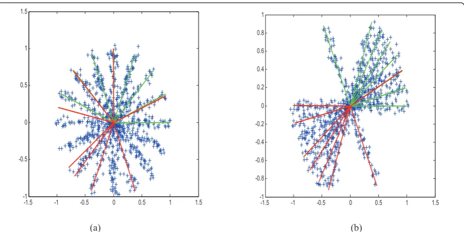
Since the traditional dictionary learning methods can be viewed as various extensions of the K-means cluster-ing method, a common drawback of them is that they are prone to local minima, i.e., the efficiency of the algo-rithms depends heavily on either the samples type or the initialization. Figure 1 shows a two-dimensional toy example in which the atom identify ability of K-SVD algorithm is investigated for two different sample types, both of which comprise of 1,000 samples and each sam-ple is a multisam-ple of one of eight basis vectors plus addi-tive noise. One type is that the dictionary’s atoms have a uniform angular distribution in the circle, and the other is that seven atoms have a uniform angular distribution in half a circle except the last one. We run K-SVD over 50 times with different realizations of coefficients and noise, and obtain the average identify ability of the two types which is 87% for the former and almost 100% for the latter. The main reason of this phenomenon is that the K-SVD algorithm is sensitive to initialization and has difficulty in updating the atom in a correct direction when the samples distribute in a directional, non-regular way. A natural way to alleviate this problem is first updating the dictionary in a low resolution or
Table 1 The denoising results in dB for six test images with noise power in the range [5,100] gray values
s/PSNR ’Barbara’ ’House’ ’Boat’ ’Lena’ ’Peppers’ ’Cameraman’
5/34.15 37.91 39.50 37.89 38.13 38.08 38.22
37.74 39.32 37.81 37.97 37.78 37.93 10/
28.13
34.19 36.05 33.58 34.30 34.59 34.00
33.94 35.97 33.39 34.02 34.17 33.71 15/
24.61
32.10 34.46 31.33 32.10 32.54 31.67
31.92 34.31 31.17 31.86 32.27 31.35 20/
22.11
30.63 33.35 29.78 30.58 31.03 30.27
30.55 33.18 29.65 30.38 30.76 29.97 25/
20.17
29.33 32.18 28.60 29.45 29.88 29.04
29.25 32.10 28.52 29.30 29.70 28.78 50/
14.15
24.57 27.76 24.98 25.83 26.20 25.73
24.65 27.85 24.99 25.76 26.19 25.65
75/ 10.61
21.50 25.19 22.67 23.55 23.69 23.38
21.52 25.26 22.72 23.56 23.72 23.38
100/ 8.13
20.19 23.46 21.66 22.02 21.90 21.70
20.26 23.40 21.67 22.01 21.86 21.72
smoothed version of the samples and then making the smoothed samples converge asymptotically to the origi-nal samples while refining the dictionary.
In this article, we propose a specific approach of such multi-scale strategy, the outline of which is to transform the constrained dictionary learning problem into the augmented Lagrangian (AL) framework first and then refine the dictionary from low scale to high. We name this approach as AL-based multi-scale dictionary learn-ing (ALM-DL) algorithm. AL is a standard and elemen-tary tool in optimization field, it converges fast even super-linearly when forcing its penalty parameter updated to infinity [22,23]. A closely related algorithm is the Bregman iterative method which was originally pro-posed by Osher et al. [24] for total variation regulariza-tion model, they are identical when the constraint is linear [25]. Under the circumstance of the study pro-posed in this article, AL is equivalent to the Bregman iterative method. We choose to follow the AL perspec-tive, instead of Bregman iteration, only because of the fact that AL is popularly used in the optimization com-munity. Usually, a “decouple” strategy (e.g., alternating direction method–ADM) is used to solve the subpro-blem of the AL scheme, it facilitates the AL to be imple-mented efficiently in many inverse problems [26-29]. In this article, we resort to a variant of this spirit. We employ a modified majorization-minimization (MM)
technique to tackle with the subproblem, enabling its solution accuracy and implementation efficiency.
The rest of the article is organized as follows: Section 2 describes the proposed method with two parts, i.e., the multi-scale dictionary learning framework and the subproblem of inner minimization. In Section 3, we conduct the experiments on synthetic data and compare its ability for recovering the original dictionary with K-SVD, MOD. Then, its ability for denoising real images is tested and compared with K-SVD in Section 4. At last Section 5 concludes the article with remarks.
2. The proposed method
This section introduces the ALM-DL algorithm for sol-ving the dictionary learning problem, it is achieved by first recasting the constrained dictionary learning pro-blem into an AL scheme, and then updating the diction-ary after each inner iteration of the scheme, during which MM technique is employed for solving the inner subproblem.
2.1 A multi-scale dictionary learning framework
In this section, l1 norm instead of l0 norm is used to relax the minimization problem Equation 2; therefore, the objective optimization problem overxinRJ is given with the subscript variable l omitted for the sake of clarity as follows
-1.5 -1 -0.5 0 0.5 1 1.5
-1 -0.5 0 0.5 1 1.5
-1.5 -1 -0.5 0 0.5 1 1.5
-1 -0.8 -0.6 -0.4 -0.2 0 0.2 0.4 0.6 0.8 1
(a) (b)
Figure 1A two-dimensional toy example testing the atom identify ability of K-SVD algorithm for two different sample types with the
min
x x1
s.t.b−Ax2≤τ
(5)
By reformulating the feasible set {x: ||b-Ax||2 ≤ τ} as an indicator function δ2τ(b−Ax), the constrained pro-blem Equation 5 turns into an unconstrained one:
min
x x1+δ 2
τ(b−Ax) (6)
whereδ2τ(z) =
0, ifz2≤τ
+∞, otherwise.
Similarly in [26,30], the resulting unconstrained blem is then converted into a different constrained pro-blem by applying a variable splitting operation, namely:
min
x,z x1+δ 2
τ(z)
s.t.−Ax−z+b= 0
(7)
We apply the method of AL for solving this con-strained problem, which is replaced by solving a sequence of unconstrained subproblems in which the objective function is formed by the original objective of the constrained optimization plus additional“penalty” terms, the“penalty”terms are made up of constrained functions multiplied by a positive coefficient (for more details of AL scheme, see [22]), i.e.,
{xk+1,zk+1}= arg min
x,z Lβ(x,z) (8)
where
yk+1=yk+ 1 2β(−Ax
k+1−zk+1+b).
yk+1=yk+ 1 2β(−Ax
k+1−zk+1+b) (9)
where〈·,·〉denotes the usual duality product.
For conventional dictionary learning approach, dic-tionary is updated after achieving the optimal minimiza-tion of Equaminimiza-tions 8 and 9 and the whole learning procedure loops in an alternative way until satisfying some conditions. In contrast, here we update dictionary after inner iteration of Equations 8 and 9, i.e., taking the derivative of functionalLbwith respect toAwe get the following gradient descent update rule:
Ak+1=Ak−μ
−Yk+ 1
2β(AkX
k+1+Zk+1−B) (Xk+1)T
=Ak+μYk+1(Xk+1)T
(10)
A merit of the AL methodology is its superior conver-gence property:Axk ® Ax* = b - z* [22], where each iterative variable“Axk“can be viewed as a low-resolution or smoothed version of the true image patches “Ax*“.
Suppose that each iterative step is regarded as a scale, then the dictionary updating, via summing the multipli-cation of primal and dual variables (i.e., Equation 10), can be seemed as a refinement process from the low scale to the high one. As discussed in the introduction, this method can avoid local optima problems because only the main features of the image patches exist at the initial stage of the iteration and we list the proposed method ALM-DL in Diagram 1.
Diagram 1. The general description of the ALM-DL algorithm
1: initiation:X0= 0;A0
2: while stop-criterion not satisfied 3: forl= 1, ...,L,{xkl+1,z
k+1
l }= arg minxl,zl Lβ(xl,zl)
Where
Lβ(xl,zl)
=xl1+δ2τ(zl)−
yk
l,Akxl+zl−bl
+ 1
4βAxl+zl−bl
2 2
4:Yk+1=Yk+ 1 2β(−AX
k+1−Zk+1+B)
5:Ak+1=Ak+μYk+1(Xk+1)T 6: end while
2.2 The sub-problem of inner minimization
From the pseudocode of the proposed algorithm depicted in Diagram 1, it is obvious that the speed and accuracy of the proposed method depend heavily on how the subproblem over variables xandz is solved, so a simple and efficient method should be developed to enable the efficiency of the whole algorithm. Ideally, the minimization of Equation 8 with respect to z can be computed analytically andzcan be eliminated:
min
z
x1+δ2τ(z)−
yk,Ax+z−b
+ 1
4βAx+z−b 2 2
=x1+ minz
δ2
τ(z) +
1 4β
Ax+z−b−2βyk2 2
=x1+ minz
δ2
τ(z) +41βz−b122
(11)
=x1+
1
4βTHτ(b1)
2
2 (12)
Denoting b1 = -Ax +b + 2byk, then the minimization of the second and third terms in Equation 11 with respect toz is obtained:
z= ⎧ ⎨ ⎩
τ
b12
b1, ifb12≥τ
b1, otherwise
THτ(b1) =b1−z= ⎧ ⎨ ⎩
b12−τ b12
b1, ifb12≥τ
Moreover, it follows that
yk+1=yk+ 1 2β(−Ax
k+1−zk+1+b)
= 1
2β
−zk+1+ (−Axk+1+b+ 2βyk)
= 1
2βTHτ
2βyk+ (b−Axk+1)
The next most crucial problem is how to determine x. It is hard to minimize Equation 11 which is nonlinear with respect to variable x, so we develop an iterative procedure to find the approximate solution. In the developed method,zis replaced by its last state zmand MM technique is employed to add an additional proxi-mal-like penalty at each inner step so as to cancel out the term ||Ax||2 (for more details of MM technique, see [31-33]). Since both of the variablesxand zare updated at each inner step, it seems justified to conclude that a satisfied solution will be obtained after just a few steps. The experimental verification is presented in Section 4.3.
xm+1= arg min x
4βx1+zm−b1 2 2+ (x−x
m)T(γI−ATA)(x−xm)
= arg min
x
4βx1+Ax−b−2βyk+zm 2 2+ (x−x
m)T
(γI−ATA)(x−xm)
= arg min
x
x−
xm+1
γAT(b+ 2βyk−zm−Axm) 2
2
+4β
γx1
= arg min
x
x1+ γ
4β
x−
xm+1
γAT(b+ 2βyk−zm−Axm) 2
2
=Shrink(xm+ 2β γATym, 2β
γ)
(13)
where g ≥ eig(AT A) and the Shrink operator is defined asShrink(f,μ) =
⎧ ⎪ ⎨ ⎪ ⎩
f −μ,f ≥μ 0, −μ≤f < μ f +μ, f <−μ
.
In summary, the proposed ALM-DL algorithm con-sists of a two-level nested loop; the outer loop updates the dual variables and the dictionary while the inner loop minimizes the primal variables at the same time to enable the accuracy of the algorithm. The detailed description of the algorithm is listed in Diagram 2, the initial dictionary A0 in line 1 can be any predefined matrix (e.g., the redundant DCT dictionary); the opera-tor THτ(Y) in line 4 implies to deal with each column of the matrixYindividually.
Diagram 2. The detailed description of the ALM-DL algorithm
1: initiation:X0= 0;A0
2: while stop-criterion not satisfied (loop ink): 3: while stop-criterion not satisfied (loop inm):
4: Ym+1= 1
2βTHτ[2βC
k−(A
kXk,m−B)]
5: Xk,m+1=shrink(Xk,m+ 2βγATkYm+1, 2βγ)
6: end while
7: Ck+1=Ym+1;Xk+1, 0=Xk, m+1 8: Ak+1=Ak+μCk+1(Xk+1, 0)T 9: end while
2.3 An hybrid method for improving performance At first glance, it seems that our proposed iterative scheme ofxm+1is very similar to the iterative shrinkage/ thresholding algorithm (ISTA), which has been inten-sively studied in the fields of compressed sensing and image recovery [10,11,25,26,28,29,32,34]. To improve the efficiency of the ISTA, various techniques have been applied to Equation 13. The most simple and fast approaches in recently years include FPC [35], SpaRSA [36], FISTA [34]. In fact, as noted in [32,34], the MM technique we employ in Section 2.2 can lead to ISTA (for details one can also see our derivation in the Appendix 1), the main novelty in our work is that we accelerate the ISTA algorithm with regard to variable xm+1
by using up-to-date zm. i.e. at each inner ISTA iteration of x, xm+1 benefits from the latest value zm. Seen from Diagram 2, by using up-to-datezm, the con-vergence of variables bothxandyare accelerated, there-fore the corresponding update of dictionaryA, Ak+1=Ak
+μYk+1(Xk+1, 0)T, are also accelerated accordingly. After this paper was submitted for publication we recently became awareaof some very recent studies by Yang [29] and Ganesh [37], the ADM framework adopted by these authors is very similar to ours, i.e. they first introduce auxiliary variables to reformulate the ori-ginal problem into the form of AL scheme, and then apply alternating minimization to the corresponding AL functions. The main differences between these method and ours lie on the fact that the application field is dif-ferent, the ultimate goal of Ganesh’s and Yang’s meth-ods in compressed sensing field pursues the sparest coefficient xunder predefined transform or dictionary, while our method is devoted to obtain the optimal dic-tionaryA.
Keep this awareness in mind, we can find the major distinction between our method and Ganesh’s and Yang’s methods. Firstly, in Yang’s study they apply the basic ISTA to solve the inner minimization with respect to variable x [[29], p. 6]. Secondly, in Ganesh’s study they apply FISTA, an accelerated technique of ISTA, to solve the inner minimization with respect to variable x [[37], pp.15-16]. Both Ganesh’s and Yang’s methods try to find sparest solution under fixed transform or dic-tionary [29,37]. Finally, in our work we aim to obtain optimal dictionary and its corresponding update form is Ak+1=Ak+μYk+1(Xk+1, 0)Tin the iterative process. This
accelerated thereby the update of dictionaryA is accel-erated. As by-products, through this modification the variablezis omitted and implicitly updated in the itera-tive scheme. Thus the whole iteraitera-tive procedure deduces to a very simple and compact iterative fashion. It is worth noting that since the number of training samples is very big for dictionary learning problem (the number adopted in the experiment of Section 4 is 62001), a sim-ple iteration formula is essential.
For comparison purpose, we modify and extend Yang’s and Ganesh’s method for dictionary learning problem by adding dictionary update stage, i.e. we update dictionary A the same as we have done in Equation 10 of Section 2.1. We call the extended Yang’s method as ADM-ISTA-DL and Ganesh’s method as ADM-FISTA-DL. The detailed description of the two methods is presented in Diagrams 3 and 4 in the Appendix 2 respectively. Furthermore, since both of our’s and Ganesh’s methods can be viewed as accelerated techniques for ISTA, we can integrate them into a unified framework for our dictionary learning problem. Diagram 5 shows the pseudocode of the hybrid algorithm. As can be seen from the Dia-gram, lines 5 and 6 come from our method which pur-sues accelerating variables xand y; on the other hand, lines 7 and 8 belonging to FISTA aim to accelerating
variable x. Compared with ADM-FISTA-DL shown in the Appendix 2, the proposed hybrid algorithm has more simple formation and faster convergence of x andy. Compared with our ALM-DL shown in Diagram 2, it inherits the strength of FISTA. To conclude, the hybrid algorithm would perform better than both, and its computational cost between our ALM-DL and ADM-FISTA-DL, the numerical comparison of the three approaches will be conducted in Section 4.3. As for real application of dictionary learning such as image denoising, we still choose the primary ALM-DL because of its simple and compact formation.
Diagram 5. The detailed description of the hybrid algorithm
1: initiation:X0= 0;A0
2: while stop-criterion not satisfied (loop ink): 3: W1=Xk;Q1 =Xk; t1 = 1
4: while stop-criterion not satisfied (loop inm):
5: Ym+1= 1
2βTHτ[2βC
k−(A
kQm−B)]
6: Wm+1=shrink(Qm+ 2βγATkYm+1, 2βγ)
7: tm+1=
1 2
1 +1 + 4t2 m
8: Qm+1=Wm+1+tm−1 tm+1
(Wm+1−Wm)
9: end while
10: Ck+1=Ym+1;Xk+1=Wm+1 11: Ak+1=Ak+μCk+1(Xk+1, 0)T 12: end while)
3. Synthetic experiments
To evaluate the proposed method, ALM-DL, we first try it on artificial data to test its ability for recovering the original dictionary and then compare it with the other two methods: K-SVD and MOD.
3.1 Test data and comparison criterion
The experiment described in [1] is repeated, first a basis AorigÎRM×Jis generated, consisting ofJ = 50 basis
vec-tors of dimension M = 20, and then 1,500 data signals {b1,b2, ...,b1500} are produced, each obtained by a linear combination of three basis vectors with uniformly dis-tributed independent identically disdis-tributed (i.i.d.) coeffi-cients in random and independent locations. We add Gaussian noise with varying SNR to the resulting data, so that we finally get the test data.
For the comparison criterion, the learned bases were gained by applying the K-SVD, MOD, and ALM-DL to the data. As in [1], we compare the learned basis with the original basis using the maximum overlap between each original basis vectoraorigj and the learned basis
vec-toralearnj , i.e., whenevermax
j
1−aorigj alearnj
is smaller than 0.01, we count this as a success [1].
Table 2 The denoising results in dB for six test images and a noise power in the range [5,100] gray values
sn ’Barbara’ ’House’ ’Boat’ ’Lena’ ’Peppers’ ’Cameraman’ 5/34.15 37.86 39.40 37.75 38.07 38.08 38.02
37.63 39.36 37.48 37.77 37.67 37.69 10/
28.13
34.29 36.10 33.61 34.28 34.54 33.92
34.08 36.07 33.34 33.93 34.16 33.41 15/
24.61
32.10 34.47 31.30 32.22 32.61 31.64
31.99 34.46 31.16 32.04 32.39 31.29 20/
22.11
30.61 33.31 29.75 30.62 31.12 30.15
30.53 33.23 29.68 30.48 30.95 29.94 25/
20.17
29.27 32.31 28.62 29.41 29.89 29.07
29.25 32.39 28.58 29.39 29.84 28.91 50/
14.15
24.82 28.20 25.07 25.83 26.29 25.70
24.90 28.11 25.11 25.80 26.26 25.65
75/ 10.61
21.80 25.24 22.76 23.46 23.52 23.61
21.71 25.20 22.74 23.45 23.49 23.58 100/
8.13
20.24 23.78 21.73 22.22 21.65 21.80
20.24 23.66 21.69 22.14 21.63 21.72
3.2 The parameter of the algorithm
The impact of parameterbon the ALM-DL algorithm is investigated in this section. In the case of SNR = 10, we setb= 0.22, 0.44, 0.66, 0.88, respectively, and run the algorithm for 180 iterations. With the process of itera-tions, we investigate the evolution of detected atom num-bers and the root mean square error (RMSE) which is defined asRMSE = 1
√
MLB−AkXk
2. As can be seen
from Figure 2, the RMSE increases but the number of successfully detected atoms (NSDA) decreases with increasingb, and an interesting phenomenon is that the larger the value ofb, the less stable the NSDA, it seems that the NSDA increases more gradually and stably when
bis very small. However, when the value of bis very small the algorithm needs more iterations. Thus, in prac-ticable implement the parameterbshould be given a relatively small value. As for the experiments conducted below, the parameterbis set as 0.45 and the number of iterationkis set as 100. For a fair comparison, the num-ber of learning iterations of K-SVD and MOD is also set to be 100, which is bigger than that in [1].
3.3 Comparison results
The ability of recovering the original dictionary is tested for three methods, namely, K-SVD, MOD, and ALM-DL, and the comparison results are given in this section. We repeat this experiment 50 times with a varying SNR of 10, 20, 30,
40, and 50 dB. As in [1], for each noise level, we sort the 50 trials according to the number of successfully learned basis elements and order them in groups of 10 experiments. Fig-ure 3 shows the results of K-SVD, MOD, and ALM-DL. As can be seen, our algorithm outperforms both of them, espe-cially when the noise level is low, ALM-DL recovers the atoms much more accurately. We know that not only the test dictionary, but also the coefficients are generated in random and independent locations, the specific distribution of the sample data widens the performance gap between our proposed ALM-DL and K-SVD. This indicates that our method has better performance on images with irregular objectives and this advantage will also be validated for real applications as shown in the next section.
4. Numerical experiments of image denoising This section presents the dictionary learned by ALM-DL algorithm and demonstrates its behavior and properties in comparison with K-SVD algorithm. We have tested our method for various denoising tests on a set of six 8-bit grayscale standard images shown in Figure 4, which are “Barbara”, “House”, “Boat”, “Lena”, “Peppers”, and
“Cameraman”. In the experiment, the whole process involves the following steps:
•Let ˆI be a corrupted version of the image I(256 × 256), after the addition of white zero-mean Gaussian noise with power sn, data examples {b1,b2, ...,b62001} of 8 × 8 pixels are extracted from the noisy imagesˆI, some
Table 3 The computation time of the four methods for running 34 iterations
ADM-ISTA-DL ADM-FISTA-DL ALM-DL The hybrid method
Boat,s= 15,m= 4 174.08s 205.45s 168.48s 188.12s Boat,s= 15,m= 7 273.39s 330.63s 279.12s 316.61s Lena,s= 15,m= 4 174.25s 207.13s 168.54s 188.29s Lena,s= 15,m= 7 271.75s 329.27s 278.75s 313.31s
0 20 40 60 80 100 120 140 160 180 0.05
0.1 0.15 0.2 0.25 0.3 0.35 0.4 0.45 0.5 0.55
Iteration
RM
S
E
E=0.22 E=0.44 E=0.66 E=0.88
0 20 40 60 80 100 120 140 160 180 200 0
5 10 15 20 25 30 35 40 45 50
Iteration
NS
D
A
E=0.22 E=0.44 E=0.66 E=0.88
(a) (b)
initial dictionary A0 is specially chosen for both of the training algorithms.
• In the sparse coding stage of learning procedure, each patch is extracted and sparse-coded. For ALM-DL we setm= 7,b= 100 and target errorτ =C√Mσnwith
the default value C = 1.15. The iteration is repeated until the error has been satisfied. Meanwhile, error-con-strained orthogonal MP (OMP) implementation is used in the K-SVD algorithm [2,38] (the K-SVD codes are available at http://www.cs.technion.ac.il/~elad/software/) to solve Equation 1 with the same target error as men-tioned above and K-SVD runs ten iterations. To enable a fair comparison, the data samples are sparse-coded using OMP under the learned dictionary for both algo-rithms after the learning procedure, these implementa-tions lead to approximate patches with reduced noise {˜b1,b˜2,· · ·,b˜62001}.
• The output image ˜I is obtained by adding the patches{˜b1,b˜2,· · ·,b˜62001}in their proper locations and
averaging the contributions in each pixel, the implemen-tation is the same as in [2].
4.1 The learned dictionary
We investigate the sensitivity of dictionaries generated by ALM-DL and K-SVD to initialization, respectively, in this section. First two dictionaries are chosen as the initializations, one is the redundant DCT dictionary (Figure 5a) and the other is a random matrix whose atom is randomly chosen from the training data (Figure 5b). Both of the dictionaries consist of J = 256 atoms and each atom is shown as an 8 × 8 pixel image. Then ALM-DL and K-SVD are used for denoising the image
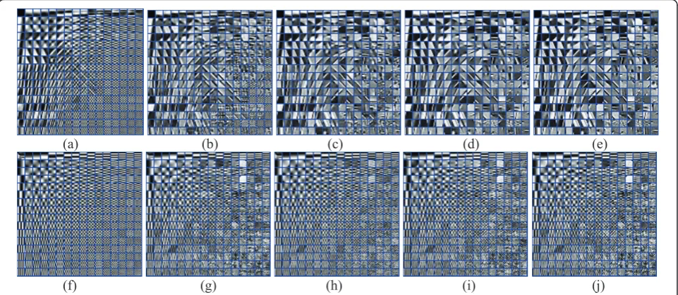
“Cameraman” withs= 10, and at last two sequences of dictionaries generated by the two methods are shown in Figures 6 and 7, respectively, from each top line of which it can be seen that the ALM-DL drastically changes the dictionary while K-SVD does not, thus the proposed algorithm has a good ability to recover the main prototypes at the first few stages. Moreover, these figures also show that the ALM-DL has another well-posed property, i.e., it is insensitive to initialization because the final learned dictionaries are very similar to each other regardless of the atom location (seen from Figures 6e and 7e), while K-SVD depends too much on the initialization. Thus, our proposed method avoids lar-gely getting trapped into some local optima.
4.2 Denoised results
In this section, ALM-DL is compared with K-SVD for the image denoising applications. In fact, the six test images in Figure 4 can be classified into two categories based on their overlapped patches’ distributions, which can be distinguished by patches’ standard covariance and principal components. The first three images (i.e.,
“Barbara”, “House”,“Boat”), typically characterized by regular textures or edges, are classified as the regular one, while the latter three images (i.e.,“Lena”,“Peppers”,
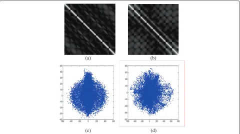
“Cameraman”), typically characterized by irregular objectives, are classified as the irregular one. Figure 8a-b shows the standard covariance matrix of the 62,001 patch examples extracted from“Barbara” and“ Camera-man”, respectively, with standard deviations= 20. The entries of the 64 × 64 matrix are between 0 and 1. As can be seen, the coordinates in 64-dimensional space of the image “Barbara” are connected more closely than
10 20 30 40 50
38 40 42 44 46 48 50
SNR (dB)
Su
cce
ss
fu
lly L
ea
rn
ed
B
asi
s E
le
m
en
ts
K-SVD MOD ALM-DL
Figure 3Comparison results of K-SVD, MOD, and ALM-DL with
respect to the reconstruction of the original basis on synthetic signals. For each of the tested algorithms and for each noise level, 50 trials were conducted and their results were sorted. The graph labels represent the mean number of successfully learned basis elements (out of 50) over the ordered tests in groups of ten experiments.
those of the image “Cameraman”. The first two-dimen-sional projection of these patch examples (through PCA transform) presented in Figure 8c-d also demonstrates the different distribution forms.
We now present denoising results obtained by our ALM-DL approach and the K-SVD method with noise level in the range of [5,100]. Every reported result is an average of over five experiments, having different reali-zations of the noise. In Table 1, the PSNRs for six test images using our ALM-DL approach are compared with the K-SVD when redundant DCT is chosen as the initial dictionary, and the best result gained by this two meth-ods are highlighted, from which we can get a conclusion that our method is better than K-SVD for all the noise levels lower than s= 25, and from Table 2 it can be seen that the conclusion is still valid when the initial dictionary is a random matrix. In order to better visua-lize their comparison, Figure 9 describes the difference
between the denoising results of the ALM-DL and K-SVD. It can be seen that our proposed approach outper-forms K-SVD for almost all the noise levels especially for the second type of images. No matter what the initial dictionary is, the PSNR value obtained by the ALM-DL gives an average advantage of 0.2 dB over K-SVD for all the noise levels lower than s= 25, but as the noise increases, the advantages of our approach is gradually weakened, and this will be a future research direction. Figure 10 plots the initial dictionary, the dic-tionary trained by K-SVD and our ALM-DL algorithm, and the corresponding denoised results of image“ Cam-eraman”withs= 15. To facilitate the visual assessment of images quality, in Figure 10d-f small regions of the physical image are boxed, in which we clearly observe the differences of the edge and the noise those images contain. It can be seen that Figure 10e shows the edge blurred but the proposed method still keeps most part of the edge. What’s more, the small boxes of Figure 10e-f also show that the K-SVD has some noise while our method does not.
The above experiments are conducted under the fixed number (i.e., J = 256) of dictionary elements, now we consider four different number of elements: 64, 128, 256, and 512. Figure 11 shows the PSNR values of image “House” and “Peppers”. As can be seen, the denoising ability of ALM-DL and K-SVD improves as the number of dictionary elements increase, while the gap of the PSNR value obtained by the two methods is bigger when the elements number is very small, which indicates that our proposed method is more robust.
(a) (b)
Figure 5 Two initial dictionary. DCT(a)and a random matrix
chosen from the training data(b).
(a) (b) (c) (d) (e)
(f) (g) (h) (i) (j)
Figure 6The dictionary learning process with DCT as initialization. From left to right: the first row: the learned dictionaries generated by
4.3 The inner sub-problem solving and its computational load
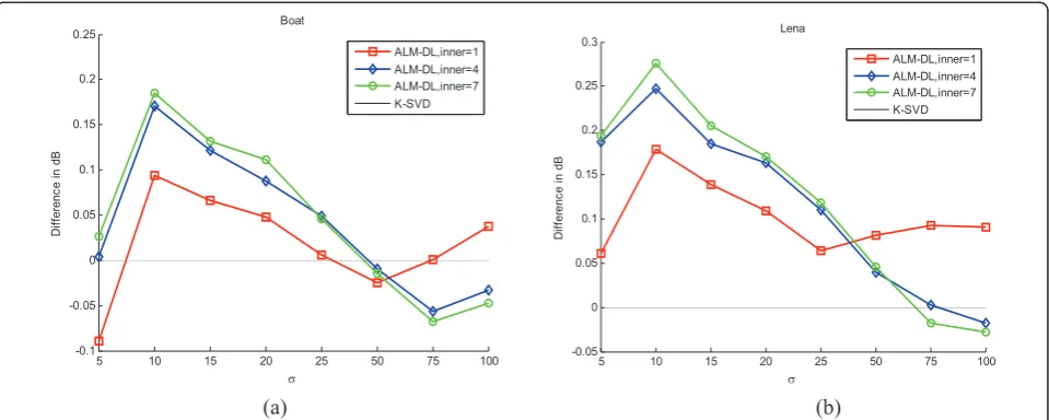
As mentioned in Section 2.2, the inner sub-problem is essential to our algorithm, so we test ALM-DL with three different inner iterations (i.e.,m= 1,4,7). Figure 12 shows
the difference of the three denoising results of ALM-DL compared with those of K-SVD, which appears as a zero straight reference line. These comparisons are presented for images‘Boat’and‘Lena’. As can be seen, the number of iterations affects the accuracy of solution very much for (a) (b) (c) (d) (e)
(f) (g) (h) (i) (j)
Figure 7The dictionary learning process with a random matrix as initialization. From left to right: the first row: the learned dictionaries
generated by ALM-DL after 2, 6, 11, 17, 20 iterations; the second row: the learned dictionaries generated by K-SVD after 1, 3, 6, 8, 10 iterations.
(a) (b)
(c) (d)
Figure 8An illustration of overlapped patches’distributions from different images. Top: the standard covariance matrix of the 62001
5 10 15 20 25 50 75 100 -0.1
0 0.1 0.2 0.3 0.4 0.5 0.6
V
Di
ff
er
enc
e i
n
dB
Barbara House Boat Lena Peppers Cameraman K-SVD
5 10 15 20 25 50 75 100
-0.1 0 0.1 0.2 0.3 0.4 0.5 0.6
V
Di
ff
er
enc
e i
n
dB
Barbara House Boat Lena Peppers Cameraman K-SVD
(a) (b)
Figure 9The difference of the denoising results between the ALM-DL and K-SVD with two initial dictionaries. The initial dictionary
whose atom is as DCT(a)and randomly chosen from the training data(b), respectively.
(a) (b) (c)
(d) (e) (f)
Figure 10The denoised result of image“Cameraman”withs= 15. Top plots:(a)the initial dictionary,(b)the dictionary trained by K-SVD,
noise levels lower thans= 25, i.e., the larger the number of iterations, the better the denoising result; and again we get the conclusion that our proposed method outperforms K-SVD much more for noise levels lower thans= 25 as demonstrated in Section 4.2. So, in practical implementa-tion of the proposed algorithm, better results are often produced with more iterations because the approximation is more accurate. However, on the other hand, more accu-rate approximates need more inner iterations and, thus, more computations. Therefore, an appropriate value ofm should be selected to trade off between accuracy and
efficiency. We suggest that selectingm= 7 as the inner iterations is a nice balance.
As we have analyzed in Section 2.3, our proposed method is very similar to Yang’s [29] and Ganesh’s [37] methods regardless of different application fields, hence we have extended them in Appendix 2 and named them as ADM-ISTA-DL and ADM-FISTA-DL, respectively, we compare them with our ALM-DL and the conse-quent hybrid algorithm. We evaluate the four methods from three criteria: RMSE, average L1norm (ALN), and the computation time, the evolution of RMSE and ALN
64 128 256 512
33.8 33.9 34 34.1 34.2 34.3 34.4 34.5
Dictionary Elements
Av
er
ag
e P
S
N
R
House
ALM-DL K-SVD
64 128 256 512
33.6 33.7 33.8 33.9 34 34.1 34.2 34.3 34.4 34.5 34.6
Dictionary Elements
Av
er
age P
S
NR
Peppers
ALM-DL K-SVD
(a) (b)
Figure 11Effect of changing the number of dictionary elements on denoising.(a)Denoising the image“House”withs= 15 and DCT as
the initial dictionary;(b)Denoising the image“Peppers”withs= 10 and a random matrix as the initial dictionary.
5 10 15 20 25 50 75 100 -0.1
-0.05 0 0.05 0.1 0.15 0.2 0.25
V
Di
ff
erenc
e i
n dB
Boat
ALM-DL,inner=1 ALM-DL,inner=4 ALM-DL,inner=7 K-SVD
5 10 15 20 25 50 75 100 -0.05
0 0.05 0.1 0.15 0.2 0.25 0.3
V
Di
ff
er
enc
e i
n
dB
Lena
ALM-DL,inner=1 ALM-DL,inner=4 ALM-DL,inner=7 K-SVD
(a) (b)
Figure 12The difference of the denoising results between the ALM-DL with iterations 1, 4, 7 and K-SVD of image“Boat”(a) and
reflect the algorithm’s effectiveness while computation time measures the algorithm’s efficiency.
Figures 13 and 14 show the RMSE and ALN of image
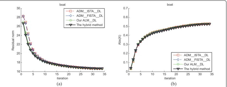
“Boat” in the case of m = 4 and m = 7, respectively. First, compared with ISTA-DL, both ADM-FISTA-DL and our ALM-DL exhibit faster convergence, with the iterative process, ADM-FISTA-DL behaves slower increase of ALN since they use FISTA in the inner minimization such that has quicker reduction of ALN under the predefined iteration number; our ALM-DL behaves faster decrease of RMSE due to the acceler-ated update of variables z and y. Second, the hybrid method outperforms the ADM-ISTA-DL, ADM-FISTA-DL, and ALM-DL. Figures 15 and 16 show the RMSE
and ALN of image“Lena”in the case ofm= 4 andm= 7, respectively, similar phenomenon is observed. Finally, from the viewpoint of computation time, Table 3 shows that our method possesses the minimum amount of time in the case of m= 4, when increasing the number of inner iteration fromm= 4 tom= 7, the computation cost of our method is a litter bigger than that of ADM-ISTA-DL. Considering all the three criteria, it concludes that our proposed approach is a very promising method.
5. Conclusions
In this article, we have developed a primal-dual-based dictionary learning algorithm under the AL framework.
The dictionary is updated by summing the
0 5 10 15 20 25 30 35
16 18 20 22 24 26 28 30
iteration
Res
idual
nor
m
boat
ADM__ISTA__DL ADM__FISTA__DL Our ALM__DL The hybrid method
0 5 10 15 20 25 30 35
0 0.1 0.2 0.3 0.4 0.5 0.6 0.7
iteration
Ab
s(X
)
boat
ADM__ISTA__DL ADM__FISTA__DL Our ALM__DL The hybrid method
(a) (b)
Figure 13The RMSE (a) and averageL1norm (ALN) (b) of four methods for image“Boat”withs= 15. The initiation dictionary is set to
DCT andm= 4.
0 5 10 15 20 25 30 35
16 18 20 22 24 26 28 30
iteration
Re
si
dual
nor
m
boat
ADM__ISTA__DL ADM__FISTA__DL Our ALM__DL The hybrid method
0 5 10 15 20 25 30 35
0 0.1 0.2 0.3 0.4 0.5 0.6 0.7
iteration
Ab
s(X
)
boat
ADM__ISTA__DL ADM__FISTA__DL Our ALM__DL The hybrid method
(a) (b)
Figure 14The RMSE (a) and averageL1norm (ALN) (b) of four methods for image“Boat”withs= 15. The initiation dictionary is set to
multiplication of primal and dual variables after each iteration of the AL scheme. The ultimate advantage of this strategy is that the proposed algorithm does not depend on the initialization too much, so it largely avoids getting trapped into some local optima. Experi-ments on image denoising application show that (1) our proposed approach outperforms the traditional alternating approaches especially for the “ Cameraman"-like images whose composite patches are distributed in a non-directional, irregular way; (2) our proposed approach is more tolerant to the number of dictionary elements, which is often unknown for signal/image processing applications.
There are several research directions that we are con-sidering currently. For instance, as proved in [22], the parameterbof the AL scheme updates in a non-increas-ing way, includnon-increas-ing the case ofb to be a constant, can guarantee its convergence. However, an automatic selec-tion of parameterbwill certainly accelerate the conver-gence, and how to achieve it remains an open question.
Appendix 1
In the appendix, we prove that the iterative scheme (13) derived by employing MM technique is essential to be an ISTA [25,32]. As mentioned in [25], the standard for-mula of ISTA for solving the general L1-minimization
0 5 10 15 20 25 30 35
27 28 29 30 31 32 33 34 35 36
iteration
Re
si
dual
nor
m
lena
ADM__ISTA__DL ADM__FISTA__DL Our ALM__DL The hybrid method
0 5 10 15 20 25 30 35
0 0.05 0.1 0.15 0.2 0.25 0.3 0.35 0.4
iteration
Ab
s(
X)
lena
ADM__ISTA__DL ADM__FISTA__DL Our ALM__DL The hybrid method
(a) (b)
Figure 15The RMSE (a) and averageL1norm (ALN) (b) of four methods for image“Lena”withs= 25. The initiation dictionary is set to
DCT andm= 4.
0 5 10 15 20 25 30 35
27 28 29 30 31 32 33 34 35 36
iteration
R
es
id
ua
l n
or
m
lena
ADM__ISTA__DL ADM__FISTA__DL Our ALM__DL The hybrid method
0 5 10 15 20 25 30 35
0 0.05 0.1 0.15 0.2 0.25 0.3 0.35
iteration
Ab
s(
X)
lena
ADM__ISTA__DL ADM__FISTA__DL Our ALM__DL The hybrid method
(b) (a)
Figure 16The RMSE (a) and averageL1norm (ALN) (b) of four methods for image“Lena”withs= 25. The initiation dictionary is set to
problem of the form:
min
x
μx1+H(x)
is
xm+1= arg min
x
μx1+
1 2δx−(x
m−δ∇H(xm))2
Settingμ= 4β; H(x) =Ax−b−2βyk+zm2
2; andδ
= 1/2g, then we give the iterative scheme (13) as fol-lows:
xm+1= arg min
x
4βx1+γ
x−
xm+1
γAT(b+ 2βyk−zm−Axm)
2
2
(13)
This is the same as we have obtained in Section 2.2.
Appendix 2
In this appendix, we modify and extend Yang’s [29] and Ganesh’s [37] methods for dictionary learning problem by adding dictionary updating stage. We are grateful to a referee for pointing out to us Yang’s [29] and Ganesh’s [37] studies. The ADM framework adopted by these authors is very similar to ours, i.e., they first introduce auxiliary variables to reformulate the original problem into the form of AL scheme, and then apply alternating minimization to the corresponding AL functions. Parti-cularly, in Yang’s study they apply ISTA to solve the inner minimization with respect to variablex [[29], p. 6], while in Ganesh’s study they apply an accelerated FISTA for solving the inner minimization instead [[37], pp. 15-16]. Although both of them try to find sparest solution under fixed dictionary, we can modify and extend them to our dictionary learning problem for comparison purpose, i.e., we update dictionary A the same as we have done in Equation 10. We call the
extended Yang’s method as ADM-ISTA-DL and
Ganesh’s method as ADM-FISTA-DL. The detailed description of the two methods is presented in Diagrams 3 and 4, respectively.
Diagram 3. The detailed description of the ADM-ISTA-DL algorithm
1: initiation:X0= 0;A0
2: while stop-criterion not satisfied (loop ink):
3: zk+1= ⎧ ⎨ ⎩
τ
b12
b1,ifb12≥τ
b1, otherwise
; b1=−Akxk+b+ 2βyk
4: while stop-criterion not satisfied (loop inm): 5: Xk,m+1=shrink(Xk,m+ 1
γAT
k(−Zk+1−AkXk,m+B+ 2βYk), 2β
γ)
6: end while
7:Xk+1=Xk, m+1;Yk+1=Yk+ 1 2β(−Z
k+1−A
kXk+1+B)
8: Ak+1=Ak+μYk+1(Xk+1)T 9: end while
Diagram 4. The detailed description of the ADM-FISTA-DL algorithm
1: initiation:X0= 0;A0
2: while stop-criterion not satisfied (loop ink):
3: zk+1=
⎧ ⎨ ⎩
τ b12
b1,ifb12≥τ
b1, otherwise
; b1 = -Ak xk +b +
2byk
4: W1=Xk;Q1=Xk;t1 = 1
5: while stop-criterion not satisfied (loop inm): 6: Wm+1=shrink(Qm+ 1
γAT
k(−Zk+1−AkQm+B+ 2βYk), 2β
γ)
7: tm+1=
1 2
1 +1 + 4t2 m
8: Qm+1=Wm+1+tm−1 tm+1
(Wm+1−Wm)
9: end while
10: Xk+1=Wm+1;Yk+1=Yk+ 1 2β(−Z
k+1−A
kXk+1+B)
11: Ak+1=Ak+μYk+1(Xk+1)T 12: end while
Endnote
a
We are grateful to a referee for pointing out to us Yang’s [29] and Ganesh’s [37] studies.
Acknowledgements
This study was partly supported by the High Technology Research Development Plan (863 plan) of P. R. China under 2006AA020805, the NSFC of China under 30670574, Shanghai International Cooperation Grant under 06SR07109, Region Rhône-Alpes of France under the project Mira Recherche 2008, and the joint project of Chinese NSFC (under 30911130364) and French ANR 2009 (under ANR-09-BLAN-0372-01). The authors are indebted to two anonymous referees for their useful suggestions and for having drawn the authors’attention to additional relevant references.
Author details 1
College of Life Science and Technology, Shanghai Jiaotong University, 200240, Shanghai, P.R. China2Department of Mathematics, Shanghai Jiaotong University, 200240, Shanghai, P.R. China
Competing interests
The authors declare that they have no competing interests.
Received: 29 July 2010 Accepted: 12 September 2011 Published: 12 September 2011
References
1. M Aharon, M Elad, AM Bruckstein, The K-SVD: an algorithm for designing of overcomplete dictionaries for sparse representations. IEEE Trans Signal Process.54(11), 4311–4322 (2006)
2. M Elad, M Aharon, Image denoising via sparse and redundant
representations over learned dictionaries. IEEE Trans Image Process.15(12), 3736–3745 (2006)
3. J Mairal, M Elad, G Sapiro, Sparse representation for color image restoration. IEEE Trans Image Process.17(1), 53–69 (2008)
5. J Mairal, F Bach, J Ponce, G Sapiro, Online dictionary learning for sparse coding, inInternational Conference on Machine Learning ICML’09(ACM, New York, 2009), pp. 689–696
6. DL Donoho, M Elad, V Temlyakov, Stable recovery of sparse over-complete representations in the presence of noise. IEEE Trans Inf. Theory.50(1), 6–18 (2006)
7. S Mallat, Z Zhang, Matching pursuits with time-frequency dictionaries. IEEE Trans Signal Process.41(12), 3397–3415 (1993). doi:10.1109/78.258082 8. JA Tropp, Greed is good: algorithmic results for sparse approximation. IEEE
Trans Inf. Theory.50(10), 2231–2242 (2004). doi:10.1109/TIT.2004.834793 9. SS Chen, DL Donoho, MA Saunders, Atomic decomposition by basis
pursuit. SIAM Rev.43(1), 129–159 (2001). doi:10.1137/S003614450037906X 10. M Elad, Why simple shrinkage is still relevant for redundant
representations? IEEE Trans Inf. Theory.52(12), 5559–5569 (2006) 11. I Gorodnitsky, B Rao, Sparse signal reconstruction from limited data using
FOCUSS: a re-weighted minimum norm algorithm. IEEE Trans Signal Process.45(3), 600–616 (1997). doi:10.1109/78.558475
12. B Efron, T Hastie, I Johnstone, R Tibshirani, Least angle regression. Ann. Statist.32(2), 407–499 (2004). doi:10.1214/009053604000000067 13. B Olshausen, D Field, Sparse coding with an overcomplete basis set: a
strategy employed by V1? Vis Res.37(23), 3311–3325 (1997). doi:10.1016/ S0042-6989(97)00169-7
14. BA Olshausen, DJ Field,Emergence of Simple-Cell Receptive Field Properties by Learning a Sparse Code for Natural Images,vol. 381. (Springer-Verlag, New York, 1996), pp. 607–609
15. K Kreutz-Delgado, J Murray, B Rao, K Engan, T Lee, T Sejnowski, Dictionary learning algorithms for sparse representation. Neural Comput.15(2), 349–396 (2003). doi:10.1162/089976603762552951
16. H Lee, A Battle, R Rajat, AY Ng, Efficient sparse coding algorithms, in
Advances in Neural Information Processing Systems 19(MIT Press, Cambridge, MA, 2007), pp. 801–808
17. K Engan, SO Aase, JH Husoy, Method of optimal directions for frame design, inIEEE International Conference Acoust., Speech, Signal Process. vol.5, 2443–2446 (1999)
18. M Yaghoobi, L Daudet, M Davies, Parametric dictionary design for sparse coding. IEEE Trans Signal Process.57(12), 4800–4810 (2009)
19. M Ataee, H Zayyani, MB Zadeh, C Jutten, Parametric dictionary learning using steepest descent, inProc. ICASSP2010(Dallas, TX, March 2010), pp. 1978–1981
20. M Zhou, H Chen, J Paisley, L Ren, G Sapiro, L Carin, Non-parametric bayesian dictionary learning for sparse image representations, inNeural Information Processing Systems (NIPS), (2009)
21. N Dobigeon, JY Tourneret, Bayesian orthogonal component analysis for sparse representation. IEEE Trans Signal Process.58(5), 2675–2685 (2010) 22. D Bertsekas,Constrained Optimization and Lagrange Multiplier Method
(Academic Press, 1982)
23. RT Rockafellar, Augmented Lagrangians and applications of the proximal point algorithm in convex programming. Math Oper Res.1(2), 97–116 (1976). doi:10.1287/moor.1.2.97
24. S Osher, M Burger, D Goldfarb, J Xu, W Yin, An iterative regularization method for total variation-based image restoration. SIAM JMMS.4, 460–489 (2005)
25. W Yin, S Osher, D Goldfarb, J Darbon, Bregman iterative algorithms for l1-minimization with applications to compressed sensing. SIAM J Imag Sci.1, 142–168 (2008). doi:10.1137/test6
26. M Afonso, J Bioucas-Dias, M Figueiredo, Fast image recovery using variable splitting and constrained optimization. IEEE Trans Image Process.19(9), 2345–2356 (2010)
27. T Goldstein, S Osher, The split Bregman method for L1-regularized problems. SIAM J Imag Sci.2(2), 323–343 (2009). doi:10.1137/080725891 28. E Esser, Applications of Lagrangian-based alternating direction methods
and connections to split Bregman, CAM Report 09-31, UCLA. (2009) 29. J Yang, Y Zhang, Alternating direction algorithms for l1 problems in
compressive sensing. Technical Report, Rice University (2009). http://www. caam.rice.edu/~zhang/reports/tr0937.pdf
30. R Tomioka, M Sugiyama, Dual augmented lagrangian method for efficient sparse reconstruction. IEEE Signal Process. Lett.16(12), 1067–1070 (2009) 31. D Hunter, K Lange, A tutorial on MM algorithms. Am Statist.58, 30–37
(2004). doi:10.1198/0003130042836
32. I Daubechies, M De Friese, C De Mol, An iterative thresholding algorithm for linear inverse problems with a sparsity constraint. Commun Pure Appl Math.57, 3601–3608 (2004)
33. J Oliveira, J Bioucas-Dias, MAT Figueiredo, Adaptive total variation image deblurring: a majorization-minimization approach. Signal Process.89(9), 1683–1693 (2009). doi:10.1016/j.sigpro.2009.03.018
34. A Beck, M Teboulle, A fast iterative shrinkage-thresholding algorithm for linear inverse problems. SIAM J Imag Sci.2(1), 183–202 (2009). doi:10.1137/ 080716542
35. E Hale, W Yin, Y Zhang, A fixed-point continuation method for L1-regularized minimization with applications to compressed sensing. CAAM Technical report TR07-07, Rice University, Houston, TX (2007)
36. S Wright, R Nowak, M Figueiredo, Sparse reconstruction by separable approximation, inProceedings of the International Conference on Acoustics, Speech, and Signal Processing(October 2008)
37. A Ganesh, A Wahner, Z Zhou, AY Yang, Y Ma, J Wright, Face recognition by sparse representation (2010), http://www.eecs.berkeley.edu/~yang/paper/ face_chapter.pdf
38. R Rubinstein, M Zibulevsky, M Elad, Efficient implementation of the K-SVD algorithm using batch orthogonal matching pursuit. Technical Report, CS Technion (2008)
doi:10.1186/1687-6180-2011-58
Cite this article as:Liuet al.:An augmented Lagrangian multi-scale dictionary learning algorithm.EURASIP Journal on Advances in Signal Processing20112011:58.
Submit your manuscript to a
journal and benefi t from:
7Convenient online submission 7Rigorous peer review
7Immediate publication on acceptance 7Open access: articles freely available online 7High visibility within the fi eld
7Retaining the copyright to your article
![Table 1 The denoising results in dB for six test imageswith noise power in the range [5,100] gray values](https://thumb-us.123doks.com/thumbv2/123dok_us/1146389.1143866/2.595.59.290.110.381/table-denoising-results-imageswith-noise-power-range-values.webp)
![Table 2 The denoising results in dB for six test imagesand a noise power in the range [5,100] gray values](https://thumb-us.123doks.com/thumbv2/123dok_us/1146389.1143866/6.595.57.291.112.381/table-denoising-results-imagesand-noise-power-range-values.webp)