Volume 2010, Article ID 287215,12pages doi:10.1155/2010/287215
Research Article
An Efficient Two-Fold Marginalized Bayesian Filter for Multipath
Estimation in Satellite Navigation Receivers
Bernhard Krach,
1Patrick Robertson,
2and Robert Weigel
31EADS Deutschland GmbH, Rechliner Straße, 85077 Manching, Germany
2The Institute of Communications and Navigation at the German Aerospace Center (DLR), Oberpfaffenhofen,
82234 Wessling, Germany
3The Chair for Electronics Engineering at the University of Erlangen-Nuremberg, Cauerstraße 9, 91058 Erlangen, Germany
Correspondence should be addressed to Bernhard Krach,[email protected]
Received 27 March 2010; Revised 4 August 2010; Accepted 17 September 2010
Academic Editor: Patrick Oonincx
Copyright © 2010 Bernhard Krach et al. This is an open access article distributed under the Creative Commons Attribution License, which permits unrestricted use, distribution, and reproduction in any medium, provided the original work is properly cited.
Multipath is today still one of the most critical problems in satellite navigation, in particular in urban environments, where the received navigation signals can be affected by blockage, shadowing, and multipath reception. Latest multipath mitigation algorithms are based on the concept of sequential Bayesian estimation and improve the receiver performance by exploiting the temporal constraints of the channel dynamics. In this paper, we specifically address the problem of estimating and adjusting the number of multipath replicas that is considered by the receiver algorithm. An efficient implementation via a two-fold marginalized Bayesian filter is presented, in which a particle filter, grid-based filters, and Kalman filters are suitably combined in order to mitigate the multipath channel by efficiently estimating its time-variant parameters in a track-before-detect fashion. Results based on an experimentally derived set of channel data corresponding to a typical urban propagation environment are used to confirm the benefit of our novel approach.
1. Introduction
Within global navigation satellite systems (GNSS), such as the Global Positioning System (GPS) or the future European satellite navigation system Galileo, the user position is determined based upon the code division multiplex access (CDMA) navigation signals received from different satellites using the time-of-arrival method [1]. A major error source for positioning comes from multipath, the reception of additional signal replicas due to reflections caused by the receiver environment. The reception of multipath introduces a bias into the time-delay estimate of the delay-lock loop (DLL) of a conventional navigation receiver, which finally leads to a bias in the receiver’s position estimate. Multipath is today still one of the most critical problems in GNSS, as the error occurs as a result of the local environment and can not be corrected through the use of correction data, which is provided by reference receiver stations or networks.
The advances in the development of signal processing techniques for multipath mitigation have led to a
conti-nual improvement of performance. Basically, two major approaches can be distinguished. Firstly, the class of tech-niques that actually mitigate the effect of multipath by modifications of the antenna pattern (either by means of hardware design or with signal processing techniques) or by aligning the more or less traditional receiver compo-nents (e.g., the early/late correlator). Secondly, the class of multipath estimation techniques, which treat multipath (in particular the delay of the paths) as something to be estimated from the received signal so that its effects can be trivially removed at a later processing stage. Most of the conventional mitigation techniques in some way align the discriminator/timing error detector of the DLL to the signal received in the multipath environment. Well-known examples of this category are, amongst others, the Narrow Correlator [2], the Strobe Correlator [3], the Gated Correlator [4], or the Pulse Aperture Correlator [5].
For the estimation techniques, static and dynamic
multipath estimation are those belonging to the family of maximum likelihood (ML) estimators, where the probably best-known technique is the multipath estimating delay-lock loop (MEDLL) [6]. In the ML approach, the signal parameters that maximize the probability of the received signal are determined. For this purpose, different maximiza-tion strategies exist, which basically characterize the different approaches. Most of these maximization algorithms are based on iterative techniques such as the Space-Alternating Generalized Expectation-Maximization algorithm (SAGE) [7, 8] and Newton-type methods. Newton-type methods have been considered with analytical [9] and numerical [10] expressions for the gradient and Hessian terms. Further ML algorithms have been reported in [11,12].
During the last years, sequential estimation algorithms in the form of Bayesian filters [13–16] have gained some attention in the field of multipath mitigation. These algo-rithms exploit prior knowledge about the temporal channel statistics through the use of statistical channel models, which allows one to improve the multipath performance of the receiver. Bayesian filters for estimation of time-varying synchronization parameters in spread spectrum systems have already been suggested in the field of communications using the extended Kalman filter [17] as well as the sequential Monte Carlo approach [18,19]. For navigation systems, an estimator based on sequential importance sampling (SIS) methods (particle filtering) was proposed in [20], which was shown to successfully mitigate multipath in a static channel scenario. An adaptation to dynamic multipath channels capable of coping with a time-variant number of multipath replicas was presented in [21]. To reduce the complexity of these approaches, it was proposed in [22] to employ reduced complexity methods for the computation of the likelihood function, which previously have been considered for ML estimation [23]. To improve the efficiency of the particle filter (PF) approach, a Rao-Blackwellized/marginalized filter was presented in [24], where the signal amplitudes are efficiently estimated via Kalman filters and where a novel proposal density for the particle filter based on a Gaussian approximation of the likelihood function was introduced. Furthermore, [24] includes a comprehensive analysis of the performance of various other Bayesian filters, and also the corresponding posterior Cramer-Rao bound (PCRB) is derived.
We believe that a key for successful application of the Bayesian approach in the future is to determine correctly the number of actually received replicas, which is unknown in practice. It is well known for the signal parameter estimation approaches that it is crucial to properly adjust the order of the employed signal model, since an improper number of degrees of freedom in the assumed model may lead to a heavy performance degradation. In previous work, however, often a known number of received replicas is assumed, and the problem of how to determine this number is not addressed [24]. To tackle this problem, we introduce in this paper a further structuring of the Bayesian approach by means of a two-fold marginalized Bayesian filter (TFMBF). The filter operates in line with filters that were presented previously, but is capable ofsimultaneously estimating all possible system
modelsin terms of the number of received multipath replicas along with their respective probabilities. We achieve this by introducing an intermediate step of marginalization, which estimates the number of impinging replicas and their parameters in a track-before-detect (TBD) fashion [25,26].
The paper is organized as follows: first, the Bayesian approach is reviewed, and the underlying signal and dynamic models are introduced. After that, we address the imple-mentation of our two-fold marginalized filter. Subsequently, we present results based upon a set of experimentally derived realistic dynamic channel data, which corresponds to a typical satellite-to-user propagation channel in urban environments [27]. Finally, we conclude the paper by a discussion of our findings.
2. The Sequential Bayesian Approach
2.1. The Sequential Bayesian Framework. For the sequential Bayesian approach, the problem of multipath mitigation becomes one ofsequential estimation of a hidden Markov pro-cess: the unknown channel parameters are estimated based on an evolving sequence of received noisy channel outputs zk. Intuitively, this concept not only exploits the observations
to estimate the hidden channel parameters but also exploits prior knowledge about the statistical dependencies between successive sets of channel parameters. The reader is referred to [13], which gives a derivation of the general framework for optimal estimation of temporally evolving parameters by means of inference viasequential Bayesian estimation. The entire history of observations up to the temporal indexkcan be written as
Zk=
zk,k=1,. . .,k. (1)
The goal is to determine thea posterioriprobability density function (PDF) of every possible channel characterization given all channel observations: p(xk | Zk), in which xk
represents the characterization of the hidden channel state. Once the a posteriori PDF is evaluated, either that channel configuration that maximizes it can be determined—the so called maximum a posteriori (MAP) estimate, or the expectation can be chosen—equivalent to the minimum mean square error (MMSE) estimate.
In the so-called prediction step,the recursive sequential Bayesian estimation algorithm computes the a priori PDF
p(xk|Zk−1) from the a posteriori PDF at time instantk−1,
p(xk−1|Zk−1) via the Chapman-Kolmogorov equation
p(xk|Zk−1)=
p(xk|xk−1)p(xk−1|Zk−1)dxk−1, (2)
with p(xk | xk−1) being the state transition PDF of the
Markov process. In theupdate step,the new a posteriori PDF for stepkis obtained via
p(xk|Zk)= p
(zk|xk)p(xk|Zk−1)
p(zk|Zk−1) .
(3)
The likelihood functionp(zk|xk) represents the probability
configuration of channel parameters at the same time step
k. To apply (2) and (3) correctly, two conditions need to be fulfilled.
(1) The noise affecting successive channel outputs is independent of the past noise values, so each channel observation depends only on the present channel state.
(2) Future channel parameters, given the present state of the channel and all its past states, depend only on the present channel state and not on any past states.
2.2. Multipath Propagation and Receiver Requirements. The typical urban multipath environment [28] poses stringent requirements on the capabilities of a receiver that is based on a parametric channel estimator, which are partially contradicting.
(i)High noise level: the power level of the received signal is usually more than 25 dB below the thermal noise, thus the algorithm has to be robust against false detection of line-of-sight (LOS) signals.
(ii)Low bandwidth: since in particular those echoes which arrive within a chip period of the CDMA signal cause the most heavy errors, the signal bandwidth is relatively low with respect to the desired timing resolution.
(iii)Multiple paths: multiple paths may impinge simul-taneously at the receiver, so the algorithm must properly determine which of them is the actual LOS path.
(iv)LOS blockage: the algorithm shall ensure that tracking of the LOS path is maintained also during periods where it is heavily attenuated.
(v)Close-in echoes: tracking of closely spaced signals with the proper multiple path signal model may lead to increased mean square errors compared to the case when tracking is based on a single-path model [29].
(vi)Track-before-detect: since it is difficult to declare dis-tinct detections of multipath replicas due to the high noise and the low signal bandwidth, the algorithm will consider the echo detection in a probabilistic fashion. The track-before-detect approach [25] is suitable for this purpose, since for any echo both hypotheses (echo present/echo not present) are esti-mated simultaneously in a probabilistic sense.
These requirements are challenging, since weak signals need to be detected and tracked properly in a noisy envi-ronment, with echoes very close to the LOS signal.
3. Channel Model
3.1. Multipath Channel Signal Model. The complex valued baseband-equivalent received signal in a navigation receiver
is assumed to be equal to
z(t)= Nm
i=0
ei(t)·ai(t)·s(t−τi(t)) +n(t), (4)
wheres(t) is the CDMA navigation signal,Nm is the maxi-mum number of considered multipath replicas reaching the receiver (to restrict the modeling complexity),ei(t)∈ {0, 1}
is a binary function that models the activity of theith path, andai(t) andτi(t) are their individual complex amplitudes and time delays, respectively. The signal is disturbed by additive white Gaussian noisen(t). The signal is sampled at times (m+kL)Ts,m = 0,. . .,L−1 and grouped in blocks ofLsamples together into vectorszk, with the block index k = 0, 1,. . .. The parameter functionsai(t),ei(t) andτi(t) are assumed to be constant and equal to ai,k, ei,k, andτi,k
for the duration of an entire block. Furthermore, the vectors τk = [τ0,k,. . .,τNm,k]
T
andak = [a0,k,. . .,aNm,k]
T
are used. The vector ek = [e0,k,. . .,eNm,k]
T determines whether the
ith path is active or not:ei,k = 1 corresponds to an active
path, and ei,k = 0 to a path that is currently not active.
In the compact form, the samples of the delayed replicas s(τi,k) are stacked together as columns of the matrixS(τk)=
[s(τ0,k),. . .,s(τNm,k)], and we may write
zk=S(τk)Ekak+nk, (5)
withEk = diag(ek). In the following, we denote the signal
hypothesis by the concise notationsk=S(τk)Ekak. Thus, we
may write according to (5) the associated likelihood function for observation blockk
p(zk|sk)=
1
(2π)Lσ2L·exp
− 1
2σ2(zk−sk)
H(
zk−sk)
,
(6)
whereσ2 refers to the variance of the elements within the
noise vectornk. The purpose of the likelihood function is
to quantify the conditional probability of the received signal conditioned on the unknown signal (specifically the channel parametersτk,ek, andak).
3.2. Markovian Channel Process Model. To exploit the advan-tages of sequential estimation for the task of multipath mitigation/estimation, the actual channel characteristics have to be described such that these are captured by p(xk |
xk−1). In other words, the model must be a first-order
Markov model, and all transition probabilities must be known. The channel state model used here is motivated by channel modeling work for multipath prone environments such as the urban satellite navigation channel [28,30]. In fact, the process of constructing a channel model in order to characterize the channel for signal level simulations and receiver evaluation comes close to our task of building a first-order Markov process for sequential estimation. Here, the channel is approximated as follows.
(ii) Each path has complex amplitudeai,kand delayτi,k,
where echoes are constrained to have delayτi,k≥τ0,k, i = 1,. . .,Nm, to reflect that multipath replicas are physically constrained to arrive later at the receiver than the LOS path.
(iii) The delay of each path follows the process
τi,k=τi,k−1+ ˙τi,k−1Δt+ni,τ+nτ (7)
with noiseni,τ,nτ, wherenτis the same value for all
indicesi.
(iv) Each parameter ˙τi,k that specifies the rate of the
change of the path delay follows its own process
˙
τi,k=τi˙,k−1+ni, ˙τ+nτ˙ (8)
with noiseni, ˙τ,nτ˙, in whichnτ˙has the same value for
all indicesi.
(v) Each echo is either “on” or “off”, as defined by the channel parameter ei,k ∈ {1 ≡ “on”, 0 ≡ “off”},
where ei,k, i = 1,. . .,Nm follows a simple
two-state Markov process with a-symmetric crossover and same-state probabilities
p ei,k=0|ei,k−1=1
=ponoff,
p ei,k=1|ei,k−1=0
=poffon.
(9)
(vi) The LOS component is always present, and conse-quentlye0,k=1 for allk.
(vii) Newly appearing echoes (ei,k=1 withei,k−1=0) are
initialized with
τi,k=τ0,k+|τm+nτ0|,
˙
τi,k=τ˙0,k+nτ˙0,
(10)
with noisenτ0,nτ˙0and the characteristic constantτm (cf. [20]).
(viii) Blockage and shadowing of the LOS signal is consid-ered through variations of the LOS amplitudea0,k.
(ix) Following [30], the complex amplitudesai,k depend
on the previous amplitudesai,k−1through
ai,k=e−j2π f0Δtτ˙i,k·ai,k−1+ni,ai, (11)
with complex noise ni,ai and the carrier frequency
f0. Thus, the rate of change in the delay affects the
evolution of the complex amplitude in a statistical manner in order to consider the physical relation-ships between phase, Doppler-frequency, and time delay adequately.
The model implicitly incorporates nine i.i.d. noise sources: Gaussianni,τ ∼N(0,σi2,τ),ni, ˙τ ∼N(0,σi2, ˙τ),nτ ∼N(0,στ2), nτ˙∼N(0,στ2˙),nτ0∼N(0,στ20),nτ˙0∼N(0,σ
2 ˙
τ0), and comp-lex Gaussianni,ai ∼ N(0,σ
2
i,ai), as well as the noise process driving the state changes forei,k. These sources provide the
randomness of the model. The noise sourcesnτandnτ˙ are
included to model the impact of the receiver clock on the individual delays and delay rates, since they are actually affected simultaneously by the same random process. Finally, Δt = LTs is the time between instants k−1 and k. It is assumed that all model parameters (i.e.,Δt, noise variances, and the “on”/“off” Markov model) are independent of k. Note that the model implicitly represents the number of actually impinging paths through the time variant parameter
Nm,k= Nm
i=0
ei,k. (12)
Using ˙τk=[ ˙τ0,k,. . ., ˙τNm,k]
T
, the hidden channel state vector xkis thus represented as
xk=[ak,ek,τk, ˙τk]. (13)
4. Estimator Implementation
Various algorithms are known which implement the Bayesian recursion (2) and (3), including the Kalman filter, the grid-based filter, and the family of particle filtering algorithms [13]. Certain restrictions are imposed on the use of these algorithms. The objective here is to estimate the channel parameters (13) via the likelihood function (6) and the channel process model defined inSection 3.2, which makes the estimation complicated: the amplitude parameters
ai,k are continuous, and the measurement depends linearly
on them like the activity parametersei,k, which are discrete
and thus follow a discrete evolution. In contrast the obser-vations depend nonlinearly on the continuous delays τi,k,
which are also nonlinear with respect to their dynamics. A straightforward way would be to implement the estimation algorithm completely with a particle filter, which is the most general method with respect to system nonlinearities, but depending on the considered number of pathsNm the state space in such a filter becomes large, and it becomes difficult to cover the entire space with a reasonable number of particles. To consider the nonlinearities while keeping the state space to be covered by the particles as small as possible, it has been proposed to reduce the computational complexity of the filter by means of marginalization over the linear state variables [16], a technique also known as Rao-Blackwellization [15]. In a marginalized filter, particles are still used to estimate the nonlinear states, while for each of the particles, the linear states can be estimated analytically. Our marginalized estimator factorizes the a posteriori density via the chain rule two-fold according to
p(ak,ek,τk, ˙τk|Zk)
=p(ak|Zk,ek,τk, ˙τk)
Kalman filter
p(ek|Zk,τk, ˙τk)
Grid-based filter
p(τk, ˙τk|Zk)
Particle filter
.
(14)
A Kalman filter is used to estimate the amplitudes ak
analytically conditional on the parameters ek, τk, and ˙τk.
using a grid-based method [13], which is appropriate to optimally estimate a discrete state space. Finally, the delays τkand the delay rates ˙τkare the only remaining parameters
that are estimated by the particle filtering algorithm. It is straightforward to show that (14) indeed corresponds to three Bayesian filters, in which the update step (3) can be expressed as
p(ak,ek,τk, ˙τk|Zk)
= p(zk|ak,ek,τk, ˙τk) p(zk|Zk−1) ·p
(ak,ek,τk, ˙τk|Zk−1)
(15)
= p(zk|ak,ek,τk, ˙τk) p(zk|Zk−1,ek,τk, ˙τk)·p
(ak|Zk−1,ek,τk, ˙τk)
Amplitude estimator: Kalman filter
(16)
·p(zk|Zk−1,ek,τk, ˙τk) p(zk|Zk−1,τk, ˙τk) ·p
(ek|Zk−1,τk, ˙τk)
Path activity estimator: grid-based filter
(17)
·p(zk|Zk−1,τk, ˙τk) p(zk|Zk−1) ·p
(τk, ˙τk|Zk−1)
Delay and delay rate estimator: particle filter
(18)
=p(ak|Zk,ek,τk, ˙τk)p(ek|Zk,τk, ˙τk)p(τk, ˙τk|Zk).
(19)
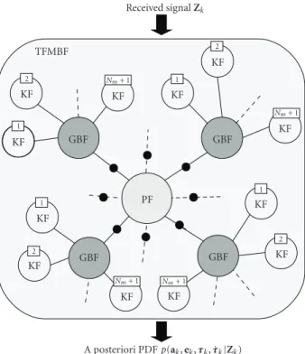
The structure of the two-fold marginalization is illus-trated inFigure 1, which reveals that the complexity of our filter is heavily dependent on the choice ofNm. However, our results that are presented inSection 5will show that with a practically reasonable choice ofNm, the complexity remains still moderate.
4.1. Estimation of Amplitudes. The implementation of the conditional amplitude filter follows from (16). The con-ditional a posteriori PDF with respect to the complex amplitudes is thus given by
p(ak|Zk,ek,τk, ˙τk)
= p(zk|ak,ek,τk, ˙τk) p(zk|Zk−1,ek,τk, ˙τk)·p
(ak|Zk−1,ek,τk, ˙τk),
(20)
in which p(zk | ak,ek,τk, ˙τk) corresponds to the likelihood
function given in (6). Recalling the structure of the mea-surement model (5), the observed signalzk is disturbed by
white Gaussian noise and depends linearly on the amplitudes ak. According to (11), the amplitude dynamics are linear
conditioned on the delay rates. Hence, (20) can be estimated with a Kalman filter and the a priori PDF for the amplitudes is given by the Gaussian density
p(ak|Zk−1,ek,τk, ˙τk)=N
a−k,P−k. (21)
Its meana−k and its covariance matrixP−k are obtained in the prediction step from the previous time instantk−1 through
the framework of the Kalman filter equations
a−k =Fkak−1, (22)
Pk−≈RFkPk−1FHk
+Q. (23)
The matrices Fk and Q follow directly from the state
transition model (11) and are computed using
Fk=diag
e−j2π f0Δtτ˙0,k,. . .,e−j2π f0Δtτ˙Nm,k
,
Q=diagσ2 0,ai,. . . ,σ
2
Nm,ai
.
(24)
The notation•above indicates that dimension and values of the respective matrices and vectors correspond to the active paths as given byek. We assume in our implementation that
(21) is still a circular symmetric complex normal PDF [31], which is enforced by the approximation via (23).
The a posteriori PDF of the amplitude filter becomes
p(ak|Zk,ek,τk, ˙τk)=N
ak,Pk
, (25)
with mean and covariance given by
ak=a−k +Kk
zk−Ska−k
,
Pk=
I−KkSk
P−k,
(26)
withSk=Sk(τk) and the Kalman gain
Kk=P−kSTk
SkP−kSTk+R
−1
. (27)
The value ofR=σ2·Ifollows directly from (6).
4.2. Estimation of Path Activity. The estimation of the path activityek follows (17), and thus the a posteriori PDF with
respect to the path activity is given by
p(ek|Zk,τk, ˙τk)
= p(zk|Zk−1,ek,τk, ˙τk) p(zk|Zk−1,τk, ˙τk) ·p
(ek|Zk−1,τk, ˙τk).
(28)
The activity state space is finite and discrete and can thus be estimated optimally using a grid-based filter [13]. In this case, the prediction (2) simplifies to the evaluation of the sum
p(ek|Zk−1,τk, ˙τk)
=
ek−1
p(ek|ek−1,Zk−1,τk, ˙τk)p(ek−1|Zk−1,τk, ˙τk).
(29)
The transition density with respect to the activity states is given by (9) and depends, therefore, on the realization of the path transitionek−1 →ek, and it can be shown that
p(ek=ek|ek−1=ek−1,Zk−1,τk, ˙τk)
=(poffon)Noffon·(ponoff)Nonoff
·(1−poffon)Noffoff·(1−ponoff)Nonon,
A posteriori PDFp(ak,ek,τk, ˙τk|Zk)
Received signalZk
KF
KF KF
KF
KF KF
KF
KF KF TFMBF
KF
KF
KF
GBF GBF
GBF GBF
PF
2
1
1
2
1 2
1
2
Nm+ 1 Nm+ 1
Nm+ 1
Nm+ 1
Figure1: Structure of the two-fold marginalized filter, which infers the a posteriori PDF of the channel parameters from the blockwise processed received signal. Each particle (black dots) of the central particle filter (PF) carries a grid-based filter (GBF) in which there are several Kalman filters (KF) according to the combination of active paths. The number of complex amplitudes to be tracked per KF (as indicated by the numbers in the boxes) ranges from 1 to
Nm+ 1.
where Noffon is the number of paths switching from “off”
to “on”,Nonoff is the number of paths switching from “on”
to “off”,Noffoff is the number of paths remaining “off”, and
Nonon is the number of paths remaining “on” during the
transition fromek−1to ek. Note that there are 2Nm discrete
states and 22Nm transitions to be covered by the grid-based filter. The marginal likelihood value used in the update step is given by the integral
p(zk|Zk−1,ek,τk, ˙τk)
=
ak
p(zk|Zk−1,ak,ek,τk, ˙τk)p(ak|Zk−1,ek,τk, ˙τk)dak.
(31)
The first term is independent of Zk−1 (6), and the second
follows from (21). This yields the Gaussian distribution
p(zk|Zk−1,ek,τk, ˙τk)=N
Ska−k,SkP−kSTk +R
. (32)
A proof for (32) can be found in [32].
4.3. Estimation of Path Delays. Due to the nonlinearity in the system model, the remaining parts of the state vector, namely, the delays and the delay rates, are to be estimated by a particle filter. Particle filters belong to the family of sequential Monte
Table1: Simulation and algorithm parameters.
Parameter Value Unit
c0 2.99792458·108 [m/s]
f0 1.57542·109 [Hz]
BHF 4 [MHz]
Ts 125 [ns]
L 80 [kSamples]
C/N0@|a0| =1 35 [db-Hz]
BDLL 1 [Hz]
BPLL 10 [Hz]
Δt 10 [ms]
Np 50
σ2
i,τ (0.03/co)2 [s]
σ2
i, ˙τ (0.03/co)2 [s/s] σ2
τ (0.03/co)2 [s]
σ2 ˙
τ (0.03/co)2 [s/s]
σ2
τ0 (100/co)
2 [s]
σ2 ˙
τ0 (0.03/co)
2 [s/s]
τm (50/co)2 [s]
poffon q
ponoff 1−q
q <0.01
σ2
i,ai 1
Carlo (SMC) filters [13], which solve the Bayesian filtering equations based on the principle ofimportance samplingand thus inherently implement only a suboptimal approximation of the optimal Bayesian solution. According to (18), the marginalized a posteriori density with respect to the path delays and delay rates is
p(τk, ˙τk|Zk)= p
(zk|Zk−1,τk, ˙τk) p(zk|Zk−1) ·
p(τk, ˙τk|Zk−1).
(33)
Here, a simple sampling importance resampling particle filter (SIR-PF) according to [14] is used to implement the marginalized delay and delay rate estimator. In the SIR-PF algorithm, the a posteriori density at stepkis represented as a sum, and is specified by a set ofNpparticles
p(τk, ˙τk|Zk)≈ Np
μ=1
wμk·δ
τk−τμk, ˙τk−τ˙ μ k
, (34)
where each particle with index μ has a state τμk, ˙τμk and has a weightwμk. Due to the marginalization, each particle
carries in addition a grid-based filter, in which for each of the discrete states a Kalman filter is associated to the particle, resulting thus in 2NmKalman filters per particle (see
Table2: Complexity of TFMBF depending onNm.
Nm NsPF NsGBF NsKF,max NKF
0 2 1 1 Np
1 4 2 2 2Np
2 6 4 3 4Np
3 8 8 4 8Np
−200
−100 0 100 200 300
Dela
y
(m)
400
0 50 100 150
Time (s)
200 250 300 350 10 20 30 40 50 60 600
500
Figure2: Typical satellite-to-pedestrian-user channel in an urban environment. The coloring indicates the power of the impinging wavefronts with respect to the receiver noise density in terms of
C/N0. The boxes highlight the channel sections that are shown subsequently in Figures6and7.
The key step of the particle filter algorithm is the calculation of the weight
wkμ∝w μ k−1
pzk|Zk−1,τμk, ˙τ μ k
pτμk, ˙τμk|τμk, ˙τμk−1
qτμk, ˙τμk|τkμ−1, ˙τμk−1,zk
, (35)
with the so-called proposal densityq(τk, ˙τk |τμk−1, ˙τ
μ k−1,zk).
In the SIR-PF, the recent measurementzkis not taken into
account by the proposal density. This choice is appropriate here, since we operate our filter in an environment that is characterized by high measurement noise, such that the likelihood function is rather flat and the dynamics of the particles are more dominant with respect to the shape of the optimal proposal density. However, other choices have been suggested in the literature, for example, a Gaussian approximation strategy [24], which may be applied as well to the particle filter employed here. The characterization of the channel process enters in the algorithm when at each time instant k the state of each particle τμk, ˙τμk is drawn randomly from the SIR-PF’s proposal distribution; that is, fromq(τk, ˙τk |τ
μ k−1, ˙τ
μ
k−1,zk)=p(τk, ˙τk |τ μ k−1, ˙τ
μ
k−1), which
corresponds to drawing values forni,τ,ni, ˙τ,nτ,nτ˙,nτ0 and
nτ˙0. As a consequence, in (35), p(τ
μ k, ˙τ
μ
k | τ
μ k−1, ˙τ
μ k−1) and
q(τμk, ˙τμk |τμk−1, ˙τμk−1,zk) cancel out, and the computation of
the new weightwμksimplifies to the evaluation of the product
20 25 30 35 40
C/
N0
(dB-Hz)
45
0 50 100 150
Time (s)
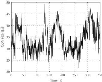
200 250 300 350 50
Figure3: Variation ofC/N0during the scenario.
0 0.1 0.2 0.3 0.5 0.6
0.4 0.7 0.8
P
robabilit
y
0.9
0
DLL RMSE=17.5 m PFNm=0, RMSE=10.8 m
PFNm=1, RMSE=6.5 m
PFNm=2, RMSE=5.4 m
PFNm=3, RMSE=4.9 m
20
10 30 40
Delay error (m)
50 60 70 80
1
Figure 4: Cumulative normalized histogram of the LOS delay estimation error of the Bayesian approach in comparison with a conventional narrow correlator DLL. Already without considering multipath, the advanced approach is significantly superior. Con-sidering more simultaneously echoes (viaNm) leads to a further
improved performance, which tends to saturate rapidly for more than one additional path.
of the previous weight and the marginalized likelihood function:wμk−1p(zk | Zk−1,τμk, ˙τ
μ
k). The marginal likelihood
value is given by summing up the marginal likelihoods over all path activity hypotheses using (32) and (29)
p(zk|Zk−1,τk, ˙τk)
=
ek
p(zk|Zk−1,ek,τk, ˙τk)p(ek|Zk−1,τk, ˙τk).
4 6 8 12 10 14 16
RSME
(m)
0
Nm=0
Nm=1
Nm=2
Nm=3
20 40
Number of particles
60 80 100
18
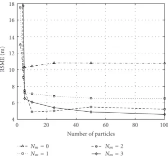
Figure5: RMSE of LOS estimate as a function of the employed number of particlesNp and the number of considered pathsNm.
Only few particles (Np<50) are needed to attain convergence.
The particle filter approach allows us to enforce the nonlinear constraint τi,k ≥ τ0,k, i = 1,. . .,Nm in an easy
way: when drawing new realizations ofτiμ,kaccording to our
proposal density via (7), we reinitializeτiμ,kand ˙τ μ
i,kaccording
to (10) in case τiμ,k < τ μ
0,k. In our implementation of the
particle filter, we apply resampling at every time instant. To tackle this potential bottleneck, advanced resampling strategies may be applied [33,34].
5. Algorithm Assessment
5.1. Scenario. To validate our algorithm, we build on the concept of thestored channel: a channel profile is recorded during a measurement campaign, and the stored profile is fed back into the receiver simulation. Though the statistical significance of such an assessment is limited, it is the most realistic approach, since the employed channel corresponds to a real world scenario. InFigure 2, the recorded channel profile from [28] which we use is illustrated. It has a total duration of 350 seconds and corresponds to a scenario, where a satellite at 10 degrees elevation transmits to a pedestrian user moving within an urban environment. The profile clearly motivates the pursued algorithmic approach. Discrete echoes due to reflectors such as house fronts are clearly visible. Thereby, each echo experiences a typical life-cycle: the reflectors cause echo traces that persist, approach, and depart along with the occasionally shadowed LOS path. Dominant channel properties are the long correlation times in the multipath echoes and their clearly observable binding to the user dynamics and the surrounding environment. The overall power variation in the channel is depicted inFigure 3. As navigation signal, we assume a GPS C/A code signal, which is a CDMA signal with a code length of 1023 (Gold code) and a chip rate of 1.023 MChips/s, such that a single
chip corresponds to a signal travel time of approximately 300 meters and the duration of an entire codeword is a millisecond. The carrier frequency of the transmitted signal is the GPS L1 center frequency f0 = 1575.42 MHz and the
receiver’s assumed reception bandwidth is BHF = 4 MHz.
Our TFMBF computes (15) at a rate of 100 Hz corresponding to Δt = 10 ms and unless stated otherwise, we employ 50 particles.
5.2. Model Matching. It is important to point out that a sequential estimator is only as good as its state transition model matches the real-world situation. The state model needs to captureallrelevant hidden states with memory and needs to correctly model their dependencies, while adhering to the first order Markov condition. Furthermore, any memory of the measurement noise affecting the likelihood function must be explicitly contained as additional states of the model, so that the measurement noise is i.i.d. Adapting the model parameters to a real channel environment is a challenging task for current and future work, since the tuning of the parameters has to take into account the potential model mismatch. The result of an adaption by empirical means, which has been the basis of the present simulations, is given inTable 1.
5.3. Results. The results of the assessment are illustrated
in Figure 4 in terms of the cumulative density function
(CDF) of the LOS estimation error when processing the entire channel scenario that is shown inFigure 2. Note that all results have been converted from signal delays to the equivalent pseudorange measures by means of the speed of light c0 and that the statistics are obtained from single
Monte Carlo trials on the 350 second scenario, respectively. Due to LOS blockage and shadowing, large errors can occur occasionally for the conventional DLL receiver, which in our case employs a standard combination of a second-order DLL with narrow correlator spacing (0.1 Chips) [2] and a loop bandwidth ofBDLL = 1 Hz and a second-order phase
locked loop (PLL) with a loop bandwidth ofBPLL =10 Hz.
−50 0 50 100
Dela
y
(m)
150 200 250
250 260 270
Time (s)
280 290 300
10 20 30 40 50 60
DLL TFMBF LOS Reference LOS
(a)Nm=0
−50 0 50 100
Dela
y
(m)
150 200 250
250 260 270
Time (s)
280 290 300
10 20 30 40 50 60
DLL TFMBF LOS
Reference LOS TFMBF MP (b)Nm=1
−50 0 50 100
Dela
y
(m)
150 200 250
250 260 270
Time (s)
280 290 300
10 20 30 40 50 60
DLL TFMBF LOS
Reference LOS TFMBF MP (c)Nm=2
−50 0 50 100
Dela
y
(m)
150 200 250
250 260 270
Time (s)
280 290 300
10 20 30 40 50 60
DLL TFMBF LOS
Reference LOS TFMBF MP (d)Nm=3
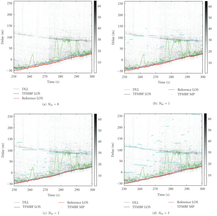
Figure6: In the illustrated scenario, there is a partially shadowed LOS path (red) that is superimposed by a heavy multipath component. During some periods with weak LOS, the DLL receiver (green) tracks the multipath signal instead of the true LOS, which leads to high errors in the order of 100 meters. The TFMBF’s LOS estimate (dark blue) is still slightly biased if the multipath replicas are not taken into account by the estimator (Nm =0, (a)). Nevertheless, the magnitude of the errors is much smaller than the DLL errors, since the dynamic model
of the estimator prevents fast variations of the LOS estimate and also because phase information is being used implicitly. Once the number of considered replicas is sufficient to take into account multipath signals (Nm>0, (b, c, d)), the estimation algorithm detects and properly
tracks the additional replicas (light blue), and thus successfully mitigates the multipath errors.
multipath and which thus are able to remove the estimation bias due to multipath, it can be observed that the estimation performance tends to saturate quickly forNm>1. Thus, the additional complexity that is needed by considering more simultaneous paths may not be justified, given the amount of performance gain. Furthermore, the rapid performance saturation forNm>1 shows that the presence of more than a
single relevant multipath component tends to happen only rarely, and if so, that the simultaneous tracking of two or more multipath replicas leads only to a small amount of performance improvement in the average error statistics.
−100
−50 0 50 100
Dela
y
(m)
150 200
30 40 50
Time (s)
60 70 80
10 20 30 40 50 60
DLL TFMBF LOS Reference LOS
(a)Nm=0
−100
−50 0 50 100
Dela
y
(m)
150 200
30 40 50
Time (s)
60 70 80
10 20 30 40 50 60
DLL TFMBF LOS
Reference LOS TFMBF MP (b)Nm=1
−100
−50 0 50 100
Dela
y
(m)
150 200
30 40 50
Time (s)
60 70 80
10 20 30 40 50 60
DLL TFMBF LOS
Reference LOS TFMBF MP (c)Nm=2
−100
−50 0 50 100
Dela
y
(m)
150 200
30 40 50
Time (s)
60 70 80
10 20 30 40 50 60
DLL TFMBF LOS
Reference LOS TFMBF MP (d)Nm=3
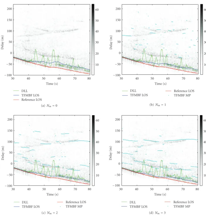
Figure7: In this scenario, the channel estimation algorithm has to cope with a LOS path (red) that is superimposed by several simultaneous multipath replicas. The DLL receiver (green) shows the typical multipath errors, whose magnitude varies due to the fading processes of the path amplitudes. If the multipath replicas are not taken into account by the estimator (Nm=0, (a)), the LOS estimate (dark blue) shows
still significant errors, but their magnitude is smaller than the DLL errors, since the dynamic model used in the estimator helps to constrain variation of the LOS estimate. WithNm=1 (b) the number of considered paths is too small to track all replicas and thus the multipath delay
estimates (light blue) tend to jump between the respective multipath signals. Once the number of considered replicas is sufficient to take into account all present signals (Nm>1, (c, d)), the estimation algorithm detects and tracks the channel, except for the period between 40 s
and 80 s. During this interval, a proper resolution of the actual LOS does not seem feasible any more, due to the presence of an echo which is born with almost zero delay w.r.t. the LOS path which itself is strongly attenuated, hence its history does not allow to separate it suitably from the LOS component.
paths Nm. The dimension of the particle filter is given by the maximum number of required multipath replicas. For the LOS path and each replicas delay and delay rate are to be estimated. Thus, the state dimension to be covered by
the particle filter is NPF
s = 2Nm + 2. Each particle needs
to carry a grid-based filter to estimate the path activities. Their respective state dimension is NGBF
s = 2Nm, because
of Kalman filters totals NKF = Np2Nm, since each activity hypothesis is required to carry its own Kalman filter. The dimension of the Kalman filters thus depends on the number of active paths and is in the range of 1,. . .,Nm+ 1. In the overall implementation, there are Np Nm
m
Kalman filters with a state dimension ofm+ 1, wheremcorresponds to the number of active echo paths. For a givenNm, the worst case state dimension of the Kalman filters is thusNKF
s,max =
Nm+ 1.Table 2summarizes these values forNm = 0,. . ., 3.
Experience with our simulations confirm that increasingNm
from 2 to 3 roughly doubles computation time. For a more detailed complexity analysis of marginalized particle filters, the reader is referred to [35].
InFigure 5, the average performance of the TFMBF is
shown as a function of the employed number of particles
Np and the parameter Nm. In contrast to previous work, the novel two-fold filter structure allows us to reduce the number of required particles significantly (cf. [22]≈20.000, [24] ≈2.000). We are able to cover the state-space more efficiently by the particles’ hypotheses, since each particle is able to exploit the carrier phase information via (11): since the complex amplitude can be measured quite precisely, we are able to infer the delay rates accurately as well. Precise delay rates in turn allow a proper prediction of the particles’ delays (7), so that in the end much fewer particles are needed to represent the a posteriori density, as the delay spread of the particles during the importance sampling is kept much smaller, since delay hypotheses, which do not match the delay rates are not generated during the importance sampling. Thus, many particles, which would be deleted during the resampling anyway and thus are a waste of computational resources, are not even generated using our approach.
5.5. Filter Behavior. To illustrate the operation of the sequen-tial estimation algorithm its MMSE estimates of the LOS and multipath delays are depicted in Figures6and7, which correspond to two typical scenarios a navigation receiver has to cope with in urban environments. The scenario illustrated
inFigure 6represents a situation where a partially shadowed
LOS component is superimposed by a strong multipath signal. The scenario shown in Figure 7 corresponds to a situation where several simultaneous echoes arrive at the receiver. The evolution of these echoes shows the typical behavior that can be observed in urban environments, including echoes that are approaching and other echoes that are departing due to the movement of the receiver towards or away from the reflector. Both scenarios reveal the general benefit of the sequential estimation approach compared to the conventional DLL. On the one hand, the explicit consideration of the multipath replicas in the signal model at the receiver allows us to mitigate the multipath errors successfully; on the other hand, the exploitation of the constrained dynamic model yields smoother and more realistic estimates, which do not follow the abrupt changes in the channel such as the DLL does occasionally; for example,
inFigure 6, during the period from 275 s to 295 s, which are
quite unlikely given the limited dynamics of the pedestrian. In particular this period shows the major drawback of the conventional DLL: though the DLL implements a low-pass
characteristic and thus limits the dynamics, it is not able to take into account a real probabilistic and physical model of the receiver dynamics and thus tends to immediately track the strongest path while neglecting any weaker earlier paths, which are much more likely to be the actual LOS path due to the recent channel history and the limited user dynamics.
6. Conclusions
In this paper, we have introduced a novel two-fold marginal-ized Bayesian filter for multipath mitigation in satellite navigation receivers. Our approach allows us to exploit the constrained channel dynamics within a typical satellite-to-user propagation scenario in an urban environment. We have proposed an efficient implementation of the filter by applying the concept of marginalization, where we proposed to estimate impinging multipath replicas in a typical track-before-detect approach. Our approach is able to adapt to the channel dynamics and favors implicitly the most likely channel configuration for a given sequence of channel observations. This has been shown to be of particular benefit in case the LOS path is shadowed or blocked, since unlike other approaches, the presented filter does not synchronize on powerful replicas during such periods. We have shown that our approach requires a significantly reduced number of particles compared to previous work, which is achieved as a result of the implicit use of phase information. Our results for a real urban environment show that our approach is practically viable and confirm its benefits. They also provide insights on how many simultaneous multipath replicas a future Bayesian navigation receiver should consider. Our findings reveal that the LOS tracking performance of our Bayesian filter tends to saturate rapidly when increasing of the number of simultaneously detectable multipath replicas.
Acknowledgments
The authors would kindly thank the anonymous reviewers for their most valuable suggestions and comments.
References
[1] E. D. Kaplan, Ed.,Understanding GPS: Principles and Applica-tions, Artech-House, Boston, Mass, USA, 1996.
[2] A. van Dierendonck, P. Fenton, and T. Ford, “Theory and performance of narrow correlator spacing in a GPS receiver,” in Proceedings of the ION National Technical Meeting, San Diego, Calif, USA, 1992.
[3] L. Garin, F. van Diggelen, and J. Rousseau, “Strobe and Edge correlator multipath mitigation for code,” inProceedings of the 9th International Technical Meeting of the Satellite Division of the Institute of Navigation (ION GPS ’96), pp. 657–664, Kansas City, Mo, USA, 1996.
[4] G. MacGraw and M. Brasch, “GNSS multipath mitigation using gated and high resolution correlator concepts,” in Proceedings of the ION National Technical Meeting, San Diego, Calif, USA, 1999.
[6] D. van Nee, J. Siereveld, P. Fenton, and B. Townsend, “The multipath estimating delay lock loop: approaching theoretical accuracy limits,” inProceedings of the IEEE Position Location and Navigation Symposium (PLANS ’94), pp. 246–251, Las Vegas, Nev, USA, 1994.
[7] J. A. Fessler and A. O. Hero, “Space-alternating generalized expectation-maximization algorithm,” IEEE Transactions on Signal Processing, vol. 42, no. 10, pp. 2664–2677, 1994. [8] F. Antreich, O. Esbri-Rodriguez, J. Nossek, and W. Utschick,
“Estimation of synchronization parameters using SAGE in a GNSS receiver,” in Proceedings of the 18th International Technical Meeting of the Satellite Division of the Institute of Navigation (ION GNSS ’05), pp. 2124–2131, Long Beach, Calif, USA, 2005.
[9] J. Selva, “An efficient Newton-type method for the compu-tation of ML estimators in a uniform linear array,” IEEE Transactions on Signal Processing, vol. 53, no. 6, pp. 2036–2045, 2005.
[10] M. Sahmoudi and M. Amin, “Fast iterative maximum-likelihood algorithm (FIMLA) for multipath mitigation in next generation of GNSS receivers,” in Proceedings of the 40th Asilomar Conference on Signals, Systems and Computers (ACSSC ’06), pp. 579–584, Pacific Grove, Calif, USA, October 2006.
[11] P. Fenton and J. Jones, “The theory and performance of NovAtel Inc.s Vision Correlator,” in Proceedings of the 8th International Technical Meeting of the Satellite Division of the Institute of Navigation (ION GNSS ’05),, pp. 2178–2186, Long Beach, Calif, USA, September 2005.
[12] L. Weill, “Achieving theoretical bounds for receiver-based multipath mitigation using Galileo OS signals,” inProceedings of the 19th International Technical Meeting of the Satellite Division of the Institute of Navigation (ION GNSS ’06), pp. 1035–1047, Fort Worth, Tex, USA, September 2006.
[13] M. S. Arulampalam, S. Maskell, N. Gordon, and T. Clapp, “A tutorial on particle filters for online nonlinear/non-Gaussian Bayesian tracking,”IEEE Transactions on Signal Processing, vol. 50, no. 2, pp. 174–188, 2002.
[14] A. Doucet, N. de Freitas, and N. Gordon, Eds., Sequential Monte Carlo Methods in Practice, Springer, New York, NY, USA, 2001.
[15] A. Doucet, N. de Freitas, K. Murphy, and S. Russell, “Rao-Blackwellised particle filtering for dynamic Bayesian net-works,” in Proceedings of the 16th Annual Conference on Uncertainty in Artificial Intelligence (UAI ’00), pp. 176–183, San Francisco, Calif, USA, 2000.
[16] T. Sch¨on, F. Gustafsson, and P.-J. Nordlund, “Marginalized particle filters for mixed linear/nonlinear state-space models,” IEEE Transactions on Signal Processing, vol. 53, no. 7, pp. 2279– 2289, 2005.
[17] R. A. Iltis, “Joint estimation of PN code delay and multipath using the extended Kalman filter,” IEEE Transactions on Communications, vol. 38, no. 10, pp. 1677–1685, 1990. [18] E. Punskaya, A. Doucet, and W. J. Fitzgerald, “Particle filtering
for joint symbol and code delay estimation in DS spread spec-trum systems in multipath environment,”EURASIP Journal on Applied Signal Processing, vol. 2004, no. 15, pp. 2306–2314, 2004.
[19] T. Bertozzi, D. Le Ruyet, C. Panazio, and H. Vu Thien, “Channel tracking using particle filtering in unresolvable multipath environments,”EURASIP Journal on Applied Signal Processing, vol. 2004, no. 15, pp. 2328–2338, 2004.
[20] P. Closas, C. Fernandez-Prades, and J. Fernandez-Rubio, “Bayesian DLL for multipath mitigation in navigation systems
using particle filters,” inProceedings of the IEEE International Conference on Acoustics, Speech and Signal Processing 2006 (ICASSP ’06), Toulouse, France, May 2006.
[21] M. Lentmaier, B. Krach, P. Robertson, and T. Thiasiriphet, “Dynamic multipath estimation by sequential Monte Carlo methods,” inProceedings of the 20th International Technical Meeting of the Satellite Division of the Institute of Navigation (ION GNSS ’07), Fort Worth, Tex, USA, September 2007. [22] M. Lentmaier, B. Krach, and P. Robertson, “Bayesian time
delay estimation of GNSS signals in dynamic multipath environments,”International Journal of Navigation and Obser-vation, vol. 2008, Article ID 372651, 11 pages, 2008.
[23] J. Selva, “Complexity reduction in the parametric estimation of superimposed signal replicas,”Signal Processing, vol. 84, no. 12, pp. 2325–2343, 2004.
[24] P. Closas, C. Fern´andez-Prades, and J. A. Fern´andez-Rubio, “A Bayesian approach to multipath mitigation in GNSS receivers,”IEEE Journal on Selected Topics in Signal Processing, vol. 3, no. 4, pp. 695–706, 2009.
[25] D. J. Salmond and H. Birch, “A particle filter for track-before-detect,” inProceedings of the American Control Conference, vol. 5, pp. 3755–3760, Arlington, Va, USA, June 2001.
[26] S. S¨arkk¨a, A. Vehtari, and J. Lampinen, “Rao-Blackwellized particle filter for multiple target tracking,”Information Fusion, vol. 8, no. 1, pp. 2–15, 2007.
[27] A. Steingass and A. Lehner, “Land mobile satellite navigation—characteristics of the multipath channel,” in Proceedings of the 16th International Technical Meeting of the Satellite Division of the Institute of Navigation (ION GNSS ’03), Portland, Ore, USA, September 2003.
[28] A. Steingass and A. Lehner, “Measuring the navigation multipath channel—a statistical analysis,” inProceedings of the 17th International Technical Meeting of the Satellite Division of the Institute of Navigation (ION GNSS ’04), pp. 1157–1164, Long Beach, Calif, USA, September 2004.
[29] P. Stoica and A. Nehorai, “MUSIC, maximum likelihood, and Cramer-Rao bound,”IEEE Transactions on Acoustics, Speech, and Signal Processing, vol. 37, no. 5, pp. 720–741, 1989. [30] A. Lehner and A. Steingass, “A novel channel model for
land mobile satellite navigation,” in Proceedings of the 18th International Technical Meeting of the Satellite Division of the Institute of Navigation (ION GNSS ’05), Fort Worth, Tex, USA, September 2005.
[31] B. Picinbono, “Second-order complex random vectors and normal distributions,”IEEE Transactions on Signal Processing, vol. 44, no. 10, pp. 2637–2640, 1996.
[32] T. Sch¨on, “On computational methods for nonlinear estima-tion,” Licentiate Thesis 1047, Department of Electrical Engi-neering, Link¨oping University, Link¨oping, Sweden, October 2003.
[33] M. Boli´c, P. M. Djuri´c, and S. Hong, “Resampling algorithms and architectures for distributed particle filters,”IEEE Transac-tions on Signal Processing, vol. 53, no. 7, pp. 2442–2450, 2005. [34] J. M´ıguez, “Analysis of parallelizable resampling algorithms for
particle filtering,”Signal Processing, vol. 87, no. 12, pp. 3155– 3174, 2007.