Volume 2007, Article ID 63219,7pages doi:10.1155/2007/63219
Research Article
Estimation of Spectral Exponent Parameter of
1/ f
Process in
Additive White Background Noise
S ¨uleyman Baykut,1Tayfun Akg ¨ul,1, 2and Semih Ergintav2
1Department of Electronics and Communications Engineering, Istanbul Technical University, 34469 Maslak, Istanbul, Turkey
2T ¨UB˙ITAK Marmara Research Center, Earth and Marine Sciences Institute, 41470 Gebze, Kocaeli, Turkey
Received 29 September 2006; Revised 5 February 2007; Accepted 29 April 2007
Recommended by Abdelhak M. Zoubir
An extension to the wavelet-based method for the estimation of the spectral exponent,γ, in a 1/ fγprocess and in the presence of additive white noise is proposed. The approach is based on eliminating the effect of white noise by a simple difference operation constructed on the wavelet spectrum. Theγparameter is estimated as the slope of a linear function. It is shown by simulations that the proposed method gives reliable results. Global positioning system (GPS) time-series noise is analyzed and the results provide experimental verification of the proposed method.
Copyright © 2007 S¨uleyman Baykut et al. This is an open access article distributed under the Creative Commons Attribution License, which permits unrestricted use, distribution, and reproduction in any medium, provided the original work is properly cited.
1. INTRODUCTION
1/ fγprocesses, also referred to as self-similar processes, are observed in many diverse fields and have gained importance in various signal processing applications from geophysical records to biomedical signals, from economical indicators to internet network traffic [1–6]. 1/ fγ processes are generally characterized by a power-law relationship in the frequency domain, that is, the empirical (or measured) power spectra of such processes are considered to be of the form [1]
Sx(ω)∼ σ
2
x
|ω|γ (1)
over some decades of frequencyω, whereσ2
x is a finite non-zero constant and γ is the so-called spectral exponent (or sometimes it is called the self-similarity parameter). In gen-eral, 1/ fγ processes can be modeled by fractional Gaussian noise (fGn) and fractional Brownian motion (fBm). fBms are zero-mean, normally distributed, nonstationary random processes with 1< γ <3, whereas fGns are zero-mean, nor-mally distributed, stationary incremental processes of fBms with−1< γ <1 [1,7]. 1/ fγprocesses are also named as col-ored noise. White noise having a flat spectrum is the special case of colored noise, where the spectral exponentγ=0. For
γ =1, it is called flicker noise and forγ =2, it is known as classical Brownian motion (random walk process).
The importance of such processes is due to the fact that they can be modeled by a single parameter γ which can be used for diagnosis, prediction, and control purposes in many applications. Therefore, an accurate estimation ofγis needed. However, estimation of this parameter is not often straightforward, especially when the data is considered to be corrupted by additive white noise. For this case, the measured power spectrumSx(ω) is
Sx(ω)∼ σ
2
x
|ω|γ +σ
2
g, (2)
whereσ2
g is the variance of the white noise. Now, estimation of the underlying characteristics of such processes becomes challenging simply because there is a single equation with more than one unknown parameter.
Although it may seem straightforward to separate a 1/ fγ -type process from additive white noise, one has to know the domination of this process among frequency regions exactly. There are several methods forγestimation from noisy mea-surements [3–5,8–11]. Among them, the conventional ones attempt to estimate the parameters of the processes in the spectral domain [3,4]. In this approach,σ2
a least-square fit algorithm to the spectrum in (2). The spec-tral density of the 1/ fγ process rapidly decays towards the higher frequency regions so that the white noise spectrum tends to dominate the rest of the spectrum which makes a reliable estimation ofγdifficult.
There are also some other methods such as approximate and exact maximum-likelihood estimation methods in the time—[3–5] and in the wavelet—[8,9,11] domains. In [3– 5], a maximization of a likelihood function is suggested in the time domain. This approach, however, is complex (i.e., matrix inversion is required) and time consuming (i.e., an it-erative technique). In [8], a parameter estimation algorithm for 1/ fγ process in white background noise based on iter-ative maximum likelihood in wavelet domain is proposed. This method, when compared with other methods, is con-sidered to have relatively low computational complexity. In [11], a modified version is utilized using the discrete wavelet transform with Haar basis.
In this paper, a simple and practical extension to the wavelet-basedγ estimation method [8] is proposed, where γis estimated directly (without iteration) by using a differ-entiation operation in the wavelet domain.
The paper is organized as follows. First, the wavelet-based γ estimation technique is briefly summarized, and then a simplified version is proposed. The effectiveness of this ex-tension is examined using synthetic data with known param-eters. The method provides promising results and GPS time series noise is analyzed to provide experimental verification.
2. WAVELET-BASEDγESTIMATION IN THE PRESENCE OF WHITE NOISE
Wavelet-basedγestimation method relies on calculating the wavelet coefficients and investigating if the variances of the wavelet coefficients follow the power-law relationship [1]. The method utilizes the orthonormal wavelet transform of a processx(t) to estimate the spectral exponent
xm n =
∞
−∞x(t)ψ
m
n(t)dt. (3)
Here,xm
n are the wavelet transform coefficients of the sig-nalx(t),nandmare the translation (location) and dilation (scale) indices, respectively.ψm
n(t) are the normalized dyadic dilations and integer translations of the mother waveletψ(t) which isψm
n(t)=2m/2ψ(2mt−n). The wavelet transform acts as the whitening process for a 1/ fγprocess where the corre-sponding wavelet coefficients appear to be zero-mean, uncor-related, or weakly correlated (within and along scales) ran-dom variables. The variances of the uncorrelated or weakly correlated wavelet coefficients along scales satisfy a power-law relationship [1]
varxnm
=σ22−γm, (4)
where σ2 is a positive real constant which is proportional
toσ2
x. In the labeling scheme used, higher scales are related
to the higher (and wide) frequency regions, whereas lower scales are related to the lower (and narrow) frequency ranges, respectively. Taking base-2 logarithm of both sides of (4) yields a straight line whose slope is the estimatedγ param-eter
log2varxm n
=c−γm. (5)
Here,cis a constant equal to log2(σ2).
If the corresponding process is corrupted by additive white noise,γcannot be estimated by a linear fit in linear-log scale. Consider the noisy processr(t) as the superposition of colored (x(t)) and white (g(t)) noise
r(t)=x(t) +g(t). (6)
The wavelet coefficients ofr(t) are obtained from (3):
rm n =
∞
−∞
x(t) +g(t)ψm
n(t)dt. (7)
In this study, the discrete dyadic wavelet transform is used to obtain the wavelet coefficients, where the number of scalesM is related with the data lengthNbyM =log2(N). Statistical independence implies that the wavelet coefficients ofr(t) are
rm
n =xnm+gnm, (8)
and the variances of these coefficients are related according to [8]
varrnm
=varxmn
+ vargnm
. (9)
The power spread of white noise is uniform throughout the entire spectrum, hence the variance of the wavelet coeffi -cients of the white noise component in each scale is equal to the variance of the white noise process (σ2
g) [1,8,11]. There-fore, considering (4), (9) becomes
σm r
2
=σ22−γm+σ2
g. (10)
In [8], a log-likelihood function is expressed as a function of the unknown parametersσ2,σ2
g, andγ. There, three cases are analyzed: (i) all of the parameters are unknown; (ii)σ2and
γ are unknown,σ2
g is known; (iii) σ2 andγ are unknown, σ2
g = 0. In the first two cases, an iterative expectation-maximization (EM) algorithm is utilized to estimate the pa-rameters. In the third case whereσ2
−6
−4
−2 0 2 4 6
log
2
(var(
x
m n))
0 2 4 6 8 10 12
m γ=1
(a)
−6
−4
−2 0 2 4 6
log
2
(
σ
2)g
0 2 4 6 8 10 12
m γ=0
(b)
−6
−4
−2 0 2 4 6
log
2
(var(
x
m n)+
σ
2)g
0 2 4 6 8 10 12
m γ1=0.7812
γ2=0.1524
(c)
−6
−4
−2 0 2 4 6
log
2
(
Δ
(
σ
m r)
2)
0 2 4 6 8 10 12
m γ=1
(d)
Figure1: Base-2 logarithm of the variances of the wavelet coefficients (a) of the processx(t) (withγ=1), (b) of white noise (γ=0), (c) of the compound signal, (d) the difference sequence of the logarithm of the variances of the wavelet coefficients in (b). (Note that the values in the figures are theoretically chosen.)
2.1. Proposed method
In this study, a simple extension is proposed to estimate the parameters directly, without using any iterative minimiza-tion technique even when white noise exists.
When γ > 0, the process has lower power at higher scales which are more affected by the white noise compo-nent than at the lower scales. Therefore, if the logarithm of both sides of (10) is taken, a curve like behavior is ob-served, instead of a straight line, as is illustrated inFigure 1 where simulation results are given for flicker noise (γ = 1) and additive white noise (γ = 0). Here, the data length is considered to be 2048. In Figures 1(a), 1(b), and 1(c), the base-2 logarithm of the variances of the wavelet
In order to estimateγ,σ2, andσ2
g directly and reliably, a difference sequence of (10) can be constructed along scales as
σm r
2
=σm r
2
−σm+1
r
2
=σ22−γm−σ22−γ(m+1) (11)
which eliminates the constant noise termσ2
g yielding
σrm
2
=σ21−2−γ2−γm. (12)
By taking the base-2 logarithm of both sides of (12),γand σ2 can be estimated by fitting a linear equation (a straight
line) in the least-square sense. Note that the slope here is identical to the slope of the linear equation in (5). Fi-nally,σ2
g can be estimated by substitutingγ andσ2 in (10). When the above operations are applied to the compound process ofFigure 1(c), the γestimation plot becomes as in Figure 1(d). Here, the slope is 1 which is equal to theγ pa-rameter of the underlying process (in this case, flicker noise).
Note that if one assumes the fit error as Gaussian dis-tributed, the line fit in the least-square sense corresponds to a maximum likelihood estimation which means that the pro-posed line regression method becomes a line fitting problem to data corrupted by Gaussian noise.
The performance of this approach is examined by simu-lations in the next section below.
3. SIMULATION RESULTS
In this section, the performance of the proposed technique is examined on synthetic data. The data set is constructed as synthesized 1/ fγprocesses superposed with white Gaussian noise having different SNR1 values from −20 dB to 20 dB,
with increments of 4 dB, and whereγvaries from 0.5 to 2.0 with increments of 0.25. In addition, the data length is set toN = 2i, whereiis varied from 10 to 14 with increments of 1. Using the wavelet-based synthesis method, the data sets ofK =100 trials are generated for each combination ofN, SNR, andγgiven above. Although the wavelet-basedγ esti-mation is shown to be empirically insensitive to the choice of the wavelet bases [8], in the simulations, among many available wavelet basis, Haar basis is used as suggested in [11].
The proposed technique is applied to each data set. Then, the mean values, the variances, and the root-mean-square (RMS) errors of the estimates are calculated. Here, RMS is defined as RMS= (1/K)Kk=1(γ−γ)2, whereγis the
theo-1SNR is defined as the ratio of the 1/ fγnoise variance to the white noise
variance (SNR=10 log10(σ2 x/σg2)).
retical,γis the estimated parameter, andKis the total num-ber of trials.
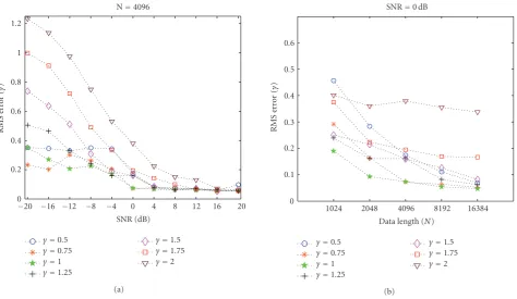
InFigure 2(a), the RMS errors of the estimatedγversus SNR values are plotted for fixed data length of 4096. We see smaller RMS errors for smallerγ(≤1) even for poor SNR(≤ 0 dB.) Whenγis relatively higher (≥1.50), the 1/ fγprocess is dominated by white noise in the high frequency regions. Notice that to have better estimates, we need to observe the logarithm of the variances of the wavelet coefficients at lower scales which requires longer data. In Figure 2(a), the RMS errors of the estimates are asymptotically bounded below as the SNR increases.
The data length dependence is observed by the results given in Figure 2(b), where the RMS errors of the esti-mated γ versus the data length N are shown for a fixed SNR value of 0 dB. Here, estimation errors decrease with the increasing data length. Note that whenγ increases, the dependency of the estimation method on the data length decreases. These results are similar to the ones given in [8,9].
In Figure 3, the mean of γ versus SNR for fixed data lengthN = 4096 is provided. For poor SNR, the method underestimates γ for larger values of γ, whereas it over-estimates γ for smaller γ. The standard deviations of the
γ estimates decrease with the increasing SNR. Note that since there are less coefficients in the small scales, the first 3 scales are not used in the γ estimation method for sta-tistical reasons. This limitation causes a bias ofγestimates for higher SNRs as is evident in Figure 3. However, when the SNR is high, the proposed technique gives similar re-sults to the noise-free case and the wavelet-based method in [8].
4. REAL DATA ANALYSIS—GPS NOISE
0 0.2 0.4 0.6 0.8 1 1.2
RMS
er
ro
r
(
γ
)
−20 −16 −12 −8 −4 0 4 8 12 16 20
N=4096
SNR (dB)
γ=0.5
γ=0.75
γ=1
γ=1.25
γ=1.5
γ=1.75
γ=2 (a)
0 0.1 0.2 0.3 0.4 0.5 0.6
RMS
er
ro
r
(
γ
)
1024 2048 4096 8192 16384 SNR=0 dB
Data length (N)
γ=0.5
γ=0.75
γ=1
γ=1.25
γ=1.5
γ=1.75
γ=2 (b)
Figure2: (a) The RMS errors of the estimatedγversus SNR for a fixed data lengthN=4096; (b) The RMS errors of the estimatedγversus various data lengthNfor SNR=0 dB.
0.5 1 1.5 2
Me
an
(
γ
)
−4 0 4 8 12 16
SNR (dB)
γ=1
γ=0.5
γ=1.5
γ=2
Figure3: The mean values of the estimatedγas a function of SNR forN=4096. The vertical lines indicate the standard deviations.
For real data, the GPS coordinate time series noise is an-alyzed. We present the analysis of the north components of GPS data obtained fromTUBI site run by T ¨UB˙ITAK Earth and Marine Sciences Institute. After the preprocessing proce-dures (outlier cleaning and small gap filling as in [3–5]), the
GPS noise is obtained as the difference (residual) between the model and the observed data. Then, the proposed technique is applied to the residual signal.
InFigure 4(a), theTUBI GPS noise data is plotted. In Figure 4(b), the base-2 logarithms of the variances of the wavelet coefficients along scales are given. The existence of white noise appears as a broken-line around the 6th scale. After applying the difference operator to the variances of the wavelet coefficients, a linear progression is observed as shown inFigure 4(c). The estimatedγvalue is close to 1 (to be exact,
γ=1.0194).
5. CONCLUSIONS
−10 0 10
(mm)
200 400 600 800 1000 1200 1400 1600
Data point (day) (a)
−2 0 2 4 6 8 10 12
log
2
(var(
r
m n))
0 2 4 6 8 10 12
Scale (m)
γ2=0.5303
γ1=1.3930
(b)
−2 0 2 4 6 8 10 12
log
2
(
Δ
(
σ
m y)
2)
0 2 4 6 8 10 12
Scale (m)
γ=1.0194
(c)
Figure4: (a) GPS noise obtained from TUBI GPS station. (b) The logarithm of the variances of the wavelet coefficients of the data in (a). Initially two different slopes of 1.3930 and 0.5303 are observed due to the white noise corruption. (c) The logarithmic difference sequence obtained from the values in (b). The spectral exponent is estimated asγ=1.0194.
Analysis of real GPS noise shows that such data can be modeled as the superposition of flicker noise (γ = 1) and white noise (γ=0), as suggested by some GPS experts.
ACKNOWLEDGMENTS
This work is supported by T ¨UB˙ITAK MRC TURDEP Project no: 5057001, EU 6. Frame Foresight Project (Contract no: 511139), and in part by T ¨UB˙ITAK CAYDAG Project no: 106Y090.
REFERENCES
[1] G. W. Wornell, “Wavelet-based representations for the 1/ f family of fractal processes,”Proceedings of the IEEE, vol. 81, no. 10, pp. 1428–1450, 1993.
[2] D. C. Agnew, “The time-domain behavior of power-law noises,”Geophysical Research Letters, vol. 19, no. 4, pp. 333– 336, 1992.
[3] J. Langbein and H. Johnson, “Correlated errors in geodetic time series: implications for time-dependent deformation,”
Journal of Geophysical Research, vol. 102, no. B1, pp. 591–604, 1997.
[4] A. Mao, C. G. A. Harrison, and T. H. Dixon, “Noise in GPS co-ordinate time series,”Journal of Geophysical Research, vol. 104, no. B2, pp. 2797–2816, 1999.
[5] S. D. P. Williams, Y. Bock, P. Fang, et al., “Error analysis of continuous GPS position time series,”Journal of Geophysical Research, vol. 109, no. B3, pp. 1–19, 2004.
[6] W. E. Leland, M. S. Taqqu, W. Willinger, and D. V. Wilson, “On the self-similar nature of Ethernet traffic (extended version),” IEEE/ACM Transactions on Networking, vol. 2, no. 1, pp. 1–15, 1994.
[7] B. B. Mandelbrot and J. W. van Ness, “Fractional Brownian motions, fractional noises and applications,” SIAM Review, vol. 10, no. 4, pp. 422–437, 1968.
[8] G. W. Wornell and A. V. Oppenheim, “Estimation of fractal signals from noisy measurements using wavelets,”IEEE Trans-actions on Signal Processing, vol. 4, no. 3, pp. 611–623, 1992. [9] B. Ninness, “Estimation of 1/ f noise,”IEEE Transactions on
Information Theory, vol. 44, no. 1, pp. 32–46, 1998.
[11] L. M. Kaplan and C.-C. J. Kuo, “Fractal estimation from noisy data via discrete fractional Gaussian noise (DFGN) and the Haar basis,” IEEE Transactions on Signal Processing, vol. 41, no. 12, pp. 3554–3562, 1993.
S¨uleyman Baykutis currently a Ph.D. can-didate and Research Assistant in the Depart-ment of Electronics and Communications Engineering at Istanbul Technical Univer-sity, Istanbul, Turkey. He received his B.S. degree (2002) in electrical-electronics en-gineering from Istanbul University, Istan-bul, Turkey, and his M.S. degree (2004) in telecommunication engineering from Istan-bul Technical University, IstanIstan-bul, Turkey.
His research interests include fractal signal processing, 1/ f (power-law) processes, noise analysis, and underwater acoustics. Part of his Ph.D. study is supported by The Scientific and Technical Research Council of Turkey (T ¨UB˙ITAK-BIDEB).
Tayfun Akg¨ulhas been a Professor at the Department of Electronics and Commu-nications Engineering in Istanbul Techni-cal University (ITU), Istanbul, Turkey, since 2002, and Chief Senior Researcher (part-time) in the Earth and Marine Sciences Institute at T ¨UB˙ITAK Marmara Research Center, Kocaeli, Turkey. His ongoing re-search is in the area of signal/image process-ing, array processprocess-ing, acoustics, speech, and
geophysical signal processing. Between 1999 and 2002, he was the Chief Senior Researcher in the Information Technologies Research Institute at T ¨UB˙ITAK Marmara Research Center. He was an Assis-tant Professor and later an Associate Professor in the Department of Electrical Engineering at C¸ukurova University in Turkey. Also, be-tween April 1997 and November 1998, he was a Visiting Assistant Professor and later a Research Associate Professor in the Electrical and Computer Engineering Department at Drexel University, USA. Between 1996 and 1997, he was a NATO postdoctoral fellow at the University of Pittsburgh. He received his Ph.D. degree in electrical engineering from the University of Pittsburgh in April 1994. He is a Senior Member of the IEEE, and currently serving as a Member-at-Large in the IEEE Publication Services and Products Board.