Earth-Abundant Materials
Thesis by
Christopher W. Roske
In Partial Fulfillment of the Requirements for the degree of
Doctor of Philosophy
CALIFORNIA INSTITUTE OF TECHNOLOGY Pasadena, California
2017
© 2017
Christopher W. Roske
Acknowledgements
This thesis would not have been possible without the tremendous support of my mentors, collaborators, peers, and friends. The National Science Foundation and Link Energy Foun-dation are thanked for generous graduate research fellowships. The NSF CCI Solar is thanked for research supplies. Forgive me for those missed below, I am short on time.
Harry Gray, Nate Lewis, Bruce Brunschwig, and (most recently) Jay Winkler have served as my staunch advisors, encouraging and supporting me in every way possible even while I have doubted myself. Harry’s positive perspective on life and science brings light to the darkest of days. Nate’s confidence in solving the hardest problems inspires scaling the tallest of scientific mountains. Bruce’s practical thinking and advice has kept me from falling too hard. I hope, one day, to reach a quarter of Jay’s breadth of knowledge. In addition, my committee has been enriched by the valuable insights of Theo Agapie and Bill Goddard.
My advisers have given me the freedom to make plenty of mistakes. Chief among those was trying to be a “One Man Army.” After years of failed ideas and projects, it took Shane Ardo’s sheer tenacity to convince me to stay, and for that I am extremely grateful. James Blakemore also left an impression on me, as is reflective of his exquisite style. I am convinced that both Shane and James will make excellent professors and I look forward to their continued success. No doubt in my mind, Wes and Aaron Sattler are busy being awesome right now.
Of labmates, Adam Nielander and Noah Plymale are my pals, and I will closely follow their progress. I really regret not getting to know Oliver Shafaat sooner, and I am excited for his future. Brian Sanders has been a welcome addition to the sub-basement crew as of late, and I hope his dreams reach fruition. Additionally, I look forward to following the progress of past and present people who have impacted my career (in the order I saw them last): Astrid Mueller (I imagine her hard efforts will yield continued success), Annelise Thompson, Jonathan Thompson, Anne Davis, James McKone, Leslie O’Leary, Donatella Bellone, and Rocio Mercado. Additionally, the help of Rick Jackson, Barbara Miralles, and Kimberly Papadantonakis has been greatly appreciated in all matters big and small.
Abstract
This thesis disembarks from the traditional approach of tailoring a system to the water splitting reaction. As detailed in Chapter 2, this thesis predicts that two silicon photoelectrons connected in parallel are ideally suited to electricity storage in an integrated light collector and chemical storage device driving the splitting of hydrobromic acid (2 HBr −−−→ H2 + Br2). The predicted dual photoelectrode
system could potentially obtain high solar-to-hydrogen conversion efficiencies of up to an ηSTH, HBr of 12 %, whereas an equivalent water splitting system is not possible due to the small band gap of silicon. Unfortunately, silicon possesses low catalytic activity for both the hydrogen evolution half-reaction and the bromide oxidation half-reaction. In the past, the electrocatalysis of silicon has been aided by using Pt/Ir alloys to act as both a protective and electrocatalytic layer. Herein, efforts are detailed to replace these precious metals, where possible, by using only earth-abundant materials to decrease the cost of a module. Our hope is that efforts along this path will aid the field of artificial photosynthesis as a whole.
We begin by further testing a chemical insight previously noted within our group and discover a surprisingly high activity electrocatalyst for the hydrogen evolution reaction by cobalt phosphide (CoP) nanoparticles, detailed in Chapter 3. Falling on a traditional technique of increasing the surface area of particular facets, we nanos-tructured our crystalline CoP to increase its surface area of exposed (111) facets and hoped it would increase our catalytic activity; however, we found that simple structuring resulted in poor adhesion of nanostructures and poorer activity than our multi-faceted CoP nanocrystals (see the appendix to find out more). Our original catalysis efforts spurred a flurry of activity in the literature, and consequently, alter-native devices that are more scalable arose. We detail the developments occurring since our work in the last appendix.
Now, with a potential catalyst in hand, comes the difficulty of balancing the delicate interplay between light absorption and catalysis, as detailed in Chapter 4. While CoP is active for HER, our particles possess a relatively low turnover frequency compared to hydrogenase or platinum, and thus require high mass loadings of ma-terial (2 mg/cm2) to obtain competitive extrinsic performance. Planar electrodes
have shown promise as potentially low-cost materials for future photovoltaic appli-cations as well as photocathodes functioning as part of an energy storage device. We discuss how to integrate our materials with silicon microwires (the wires were grown by an unscalable process to serve in place of functional CVD wires with radial emitters) to prototype a candidate photocathode. While a parasitic resistance limited the overall efficiency of the photocathode candidate, it still had promising stability. The parasitic resistance was addressed by electrodepositing the cobalt phosphide, thereby giving us a promising efficiency limited by the quality of the p-n junction.
Published Content and Contributions
(1) J. Callejas, C. G. Read, C. W. Roske, N. S. Lewis and R. E. Schaak,Chem. Mater., 2016,99, 99,
(used in Appendix K) CWR wrote section on integration.
(2) C. W. Roske, J. W. Lefler and A. M. Muller,J. Colloid Interface Sci., 2016, 00, 00,
(used in Appendix I) CWR participated in the characterization and writing of the manuscript.
(3) A. C. Nielander, A. C. Thompson, C. W. Roske, J. A. Maslyn, Y. Hao, N. T. Plymale, J. Hone and N. S. Lewis,Nano Lett., 2016,16, 4082–6,
(used in Chapter 5) CWR participated in the conception of the project and performed experiments relating to hydrobromic acid.
(4) C. W. Roske, E. J. Popczun, B. Seger, C. G. Read, T. Pedersen, O. Hansen, P. C. Vesborg, B. S. Brunschwig, R. E. Schaak, I. Chorkendorff, H. B. Gray and N. S. Lewis,J. Phys. Chem. Lett., 2015,6, 1679–83,
(used in Chapter 4) CWR conceptualized the project, performed all the major experiments, and wrote the manuscript.
(5) E. J. Popczun, C. W. Roske, C. G. Read, J. C. Crompton, J. M. McEnaney, J. F. Callejas, N. S. Lewis and R. E. Schaak, J. Mater. Chem. A, 2015, 3,
5420–5425,
(used in Appendix E) CWR participated in the characterization of electro-catalytic behavior and editing of the manuscript.
(6) L. E. O’Leary, N. C. Strandwitz, C. W. Roske, S. Pyo, B. S. Brunschwig and N. S. Lewis,J. Phys. Chem. Lett., 2015,6, 722–726,
(used in Appendix G) CWR participated in surface synthesis, characteriza-tion, and editing of the manuscript.
(7) E. J. Popczun, C. G. Read, C. W. Roske, N. S. Lewis and R. E. Schaak,
Angew. Chem., 2014,126, 5531–5534,
Table of Contents
Acknowledgements . . . iii
Abstract . . . iv
Published Content . . . vi
Table of Contents . . . vii
List of Illustrations . . . x
List of Tables . . . xiv
Chapter I: Introduction . . . 1
1.1 Motivation . . . 1
1.2 Limits of Fossil Fuels . . . 3
1.3 Greenhouse Gas Effects . . . 8
1.4 Low CO2Emission Energy Systems . . . 16
1.5 Theme of Thesis: Intermittent Energy Storage . . . 23
1.6 References . . . 25
Chapter II: System Concept . . . 28
2.1 Project Illinois . . . 28
2.2 Limits of Solar Energy Power Generation . . . 32
2.3 Basis Set of Parameters to Model Solar Cells . . . 39
2.4 Butler–Volmer Kinetic Model Effects on Ideal Diode . . . 43
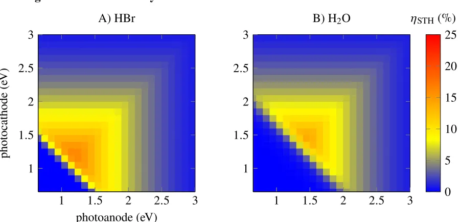
2.5 Comparison of Estimated Device Efficiencies for HBr and H2O Splitting 45 2.6 Proposed Device Layout . . . 49
2.7 Challenges Facing HBr Splitting . . . 51
2.8 Conclusions . . . 52
2.9 References . . . 53
Chapter III: Highly Active Electrocatalysis of the Hydrogen-Evolution Reac-tion by Cobalt Phosphide Nanoparticles . . . 54
3.1 Abstract . . . 54
3.2 Introduction . . . 54
3.3 Materials and Methods . . . 55
3.4 Results and Discussion . . . 55
3.5 Conclusion . . . 61
3.6 Acknowledgements . . . 62
3.7 References . . . 62
Chapter IV: Comparison of the Performance of CoP-Coated and Pt-Coated Radial Junction n+p-Silicon Microwire-Array Photocathodes for the Sunlight-Driven Reduction of Water to H2(g) . . . 64
4.1 Abstract . . . 64
4.2 Introduction . . . 65
4.3 Results and Discussion . . . 66
4.5 Acknowledgements . . . 74
4.6 References . . . 74
Chapter V: Lightly Fluorinated Graphene as a Protective Layer for n-Type Si(111) Photoanodes in Aqueous Electrolytes . . . 76
5.1 Abstract . . . 76
5.2 Introduction . . . 77
5.3 Materials and Methods . . . 78
5.4 Results and Discussion . . . 79
5.5 Conclusion . . . 84
5.6 Acknowledgements . . . 84
5.7 References . . . 84
Chapter VI: Summary . . . 87
Appendix A: Efficiency Calculation Matlab Program . . . 90
A.1 Realistic Calculation Results . . . 90
A.2 Script Dependencies . . . 91
A.3 Source Code . . . 91
Appendix B: Supplementary Information for Highly Active Electrocatalysis of the Hydrogen-Evolution by Cobalt Phosphide Nanoparticles . . . 122
B.1 Materials and Methods . . . 122
B.2 Supporting Data . . . 126
B.3 References . . . 127
Appendix C: Supplementary Information for Comparison of the Performance of CoP-Coated and Pt-Coated Radial Junction n+p-Silicon Microwire-Array Photocathodes for the Sunlight-Driven Reduction of Water to H2(g) 129 C.1 Methods . . . 129
C.2 Supplementary Data . . . 132
C.3 References . . . 135
Appendix D: Supplementary Information for Lightly Fluorinated Graphene as a Protective Layer for n-Type Si(111) Photoanodes in Aqueous Electrolytes 136 D.1 Methods . . . 136
D.2 Supporting Data . . . 140
D.3 References . . . 157
Appendix E: Highly Branched Cobalt Phosphide Nanostructures for Hydrogen-Evolution Electrocatalysis . . . 158
E.1 Abstract . . . 158
E.2 Introduction . . . 158
E.3 Experimental . . . 160
E.4 Results and Discussion . . . 162
E.5 Conclusion . . . 168
E.6 Acknowledgements . . . 169
E.7 References . . . 169
Appendix F: Supplementary Information for Highly Branched Cobalt Phos-phide Nanostructures for Hydrogen Evolution Electrocatalysis . . . 171
F.1 Additional Experimental Details . . . 171
F.3 References . . . 175
Appendix G: Use of Mixed CH3– /HC(O)CH2CH2– Si(111) Functionality to Control Interfacial Chemical and Electronic Properties During the Atomic Layer Deposition of Ultrathin Oxides on Si(111) . . . 176
G.1 Abstract . . . 176
G.2 Introduction . . . 176
G.3 Materials and Methods . . . 177
G.4 Results and Discussion . . . 178
G.5 Conclusion . . . 183
G.6 Acknowledgements . . . 183
G.7 References . . . 183
Appendix H: Supplementary Information for Use of Mixed CH3– /HC(O)CH2CH2– Si(111) Functionality to Control Interfacial Chemical and Electronic Properties During the Atomic Layer Deposition of Ultrathin Oxides on Si(111) . . . 186
H.1 Calculation of Surface Coverage from X-ray Photoelectron Spectra . 186 H.2 Microwave Conductivity Measurements . . . 187
H.3 Supporting Data . . . 187
H.4 References . . . 188
Appendix I: Complex Nanomineral Formation Utilizing Kinetic Control by PLAL . . . 189
I.1 Abstract . . . 189
I.2 Introduction . . . 189
I.3 Experimental Section . . . 190
I.4 Foil Target Setup . . . 192
I.5 Results and Discussion . . . 194
I.6 Conclusion . . . 203
I.7 Acknowledgments . . . 203
I.8 References . . . 204
Appendix J: Supplementary Information for Complex Nanomineral Forma-tion Utilizing Kinetic Control by PLAL . . . 207
Appendix K: Synthesis, Characterization, and Properties of Metal Phosphide Catalysts for the Hydrogen-Evolution Reaction . . . 208
K.1 Abstract . . . 208
K.2 Introduction . . . 208
K.3 Overview of Metal Phosphides . . . 215
K.4 Synthesis of Metal Phosphides . . . 216
K.5 Characterization of Transition Metal Phosphides for the Hydrogen-Evolution Reaction . . . 220
K.6 Transistion Metal Phosphides for the HER . . . 226
K.7 Integration with Light Absorbers . . . 251
K.8 Conclusions . . . 259
K.9 Acknowledgments . . . 259
List of Illustrations
Number Page
1.1 BP Whiting Oil Refinery . . . 2
1.2 Logistic Consumption of Total Carbon . . . 7
1.3 Logistic Consumption of Proven Fossil Fuels . . . 8
1.4 Black Body Emissions of Earth . . . 12
1.5 CO2Gas Concentration and Forcing Relationship . . . 13
1.6 Comparison Between AM0 and Black Body Emission of Sun . . . . 21
2.1 TI Solar Chemical Converter Cross Section . . . 31
2.2 Photon Flux Density AM1.5D . . . 33
2.3 Efficiency Estimates of Yield, Potential, and Power . . . 39
2.4 PredictedVocvs band gap . . . 40
2.5 Predicted Jsc vs band gap . . . 41
2.6 Predicted Silicon Solar Cell J–V Curve . . . 42
2.7 Predicted Silicon Solar Cell J–V Curve With Catalysis . . . 44
2.8 Single-Absorber Device Configuration Ideal Efficiencies . . . 46
2.9 Side-by-Side Device Configuration Ideal Efficiencies . . . 47
2.10 Tandem Configuration Device Ideal Efficiencies . . . 49
2.11 Proposed Device . . . 51
3.1 TEM, SAED, and HRTEM of CoP Nanoparticles . . . 57
3.2 Powder XRD patterns for CoP . . . 58
3.3 Polarization Data for CoP . . . 59
3.4 Polarization Stability Data for CoP . . . 61
4.1 SEM of Microwires for Photocathode . . . 67
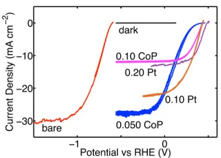
4.2 Catalyst Loading Effects . . . 68
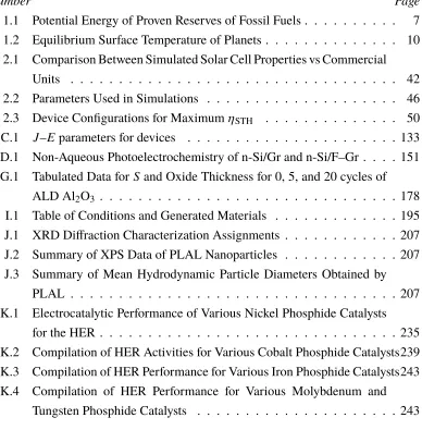
4.3 CV Behavior of Pt- or CoP-coated Photocathodes . . . 69
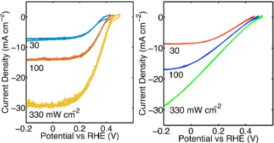
4.4 Stability of Photocathode with CoP . . . 72
4.5 J–V Behavior for Electrodeposited CoP on MWs . . . 73
5.1 CV Behavior of Graphene Protected Anodes in Fe(CN)6 . . . 82
5.2 XP spectra of Graphene electrodes. . . 83
5.3 CV Behavior of Photoanode for Br– Oxidation . . . 83
A.1 Single-Absorber Device Configuration Real Efficiencies . . . 90
A.3 Tandem Configuration Real Device Efficiencies . . . 91
B.1 TEM and PXRD for-Co nanoparticles . . . 126
B.2 EDS data for CoP nanoparticles . . . 127
B.3 XPS data for CoP/Ti electrode . . . 127
C.1 TEM of Pt nanoparticles . . . 133
C.2 XRD and TEM of CoP nanoparticles . . . 133
C.3 Spectral Response for Pt- and CoP-Coated Photoelectrodes . . . 134
C.4 Dependence of Photocurrent on Angle . . . 134
D.1 Stability Behavior of np+Photoelectrode Protected by F–Gr in Fe(CN)6141 D.2 Representative Comparison between n-Si/Gr and n-Si/F–Gr Stability 143 D.3 Representative n-Si/F–Gr Initial Decay . . . 143
D.4 Stability Comparison for Champion n-Si/Gr and n-Si/F–Gr . . . 144
D.5 Comparison of Stability Between n-Si/Gr and n-Si/F–Gr at 1 Sun Illumination Intensity . . . 145
D.6 Decay of n-Si/F–Gr over 100,000 s at 1 Sun . . . 145
D.7 Raman and XPS Data Before and After Annealing of F–Gr . . . 146
D.8 Chemical Stability Test of F–Gr in Acidic, Basic, and Neutral pH . . 147
D.9 Optical Imaging of F–Gr After Stability Test . . . 148
D.10 UV/vis Spectra of Gr and F–Gr on Glass . . . 149
D.11 Testing Formation of Platinum Silicide . . . 150
D.12 HBr J–EBehavior with F–Gr . . . 151
D.13 Shunt Resistance of F–Gr . . . 153
D.14 SEM of n-Si/F–Gr Prior to Pt Electrodeposition . . . 155
D.15 SEM of n-Si/F–Gr After 10 mC/cm2Pt Electrodeposition . . . 155
D.16 SEM of n-Si/F–Gr After 100 mC/cm2Pt Electrodeposition . . . 156
E.1 TEM and SAED Pattern of Highly Branched CoP Nanostructures . . 163
E.2 SEM of Highly Branched CoP Nanostructures . . . 163
E.3 HRTEM of CoP Nanostructure . . . 164
E.4 XRD Pattern of CoP Nanostructures . . . 165
E.5 Schematic of High Density (111) Facets of Branched CoP Nanos-tructures . . . 166
E.6 Polarization Data of CoP Nanostructures . . . 167
F.1 EDS of CoP Nanostructures . . . 172
F.2 PXRD of CoP Nanostructures on Ti Foil . . . 173
F.3 LSV of CoP Nanostructures on Ti Foil . . . 173
G.1 Synthesis of Monolayer for Metal Oxide Nucleation . . . 178
G.2 XPS of Al2O3ALD Deposition . . . 179
G.3 XPS of Surfaces after ALD of MnO . . . 180
G.4 SRV Traces for Monolayers . . . 181
G.5 ALD Growth Rates per Cycle . . . 182
G.6 Comparison of AFM Images After 20 Cycles of ALD . . . 182
H.1 Comparison of AFM Images After 5 Cycles of ALD . . . 188
I.1 PLAL Schematic . . . 194
I.2 XRD of Cu, CuO Nanoparticles . . . 196
I.3 XRD of Cu2Cl(OH)3Nanoparticles . . . 197
I.4 XRD of Cu2(NO3)(OH)3Nanoparticles . . . 198
I.5 XRD of Zn, ZnO Nanoparticles . . . 199
I.6 XRD of Zn5(OH)8Cl2·H2O Nanoparticles . . . 200
I.7 XRD of Zn5(OH)8(NO3)2·2 H2O Nanoparticles . . . 201
I.8 XRD of Cu3(Cu, Zn)Cl2(OH)6Nanoparticles . . . 203
K.1 “The Liz” . . . 210
K.2 Representative Crystal Structure Types of Metal Phosphides . . . 216
K.3 Representative Metal Phosphide Material Forms . . . 219
K.4 Polarization Data for the HER in 0.5 M H2SO4using Pt Electrodes. . 221
K.5 Summary of Methods . . . 224
K.6 Characterization of Ni2P . . . 228
K.7 Additional Examples of Ni2P . . . 229
K.8 Examples of Ni5P4 . . . 231
K.9 Crystal Structure Dependence on Ni:P Ratio . . . 232
K.10 Forms of NixPy . . . 233
K.11 CoP Examples . . . 236
K.12 CoP Polarization Data . . . 237
K.13 Characterization of Electrodeposited CoP . . . 238
K.14 Comparison Between CoP and Co2P . . . 240
K.15 FeP Characterization . . . 241
K.16 Characterization of MoP Nanoparticles . . . 244
K.17 Characterization of WP Nanoparticles . . . 245
K.18 Characterization of Copper Phosphide Nanostructures . . . 246
K.19 Polarization Data for Several Transition Metal Phosphides . . . 247
K.20 Characterization of MoP|S . . . 249
K.22 Optimized Structures for the (001) Surface of Ni2P . . . 251
K.23 ηSTH for Single and Tandem Configuration of Light Absorbers for Water Splitting . . . 252
K.24 Microwires for Photocathode . . . 254
K.25 Micropyramid-Structured Silicon Photocathode . . . 255
List of Tables
Number Page
1.1 Potential Energy of Proven Reserves of Fossil Fuels . . . 7
1.2 Equilibrium Surface Temperature of Planets . . . 10
2.1 Comparison Between Simulated Solar Cell Properties vs Commercial Units . . . 42
2.2 Parameters Used in Simulations . . . 46
2.3 Device Configurations for MaximumηSTH . . . 50
C.1 J–Eparameters for devices . . . 133
D.1 Non-Aqueous Photoelectrochemistry of n-Si/Gr and n-Si/F–Gr . . . . 151
G.1 Tabulated Data for Sand Oxide Thickness for 0, 5, and 20 cycles of ALD Al2O3 . . . 178
I.1 Table of Conditions and Generated Materials . . . 195
J.1 XRD Diffraction Characterization Assignments . . . 207
J.2 Summary of XPS Data of PLAL Nanoparticles . . . 207
J.3 Summary of Mean Hydrodynamic Particle Diameters Obtained by PLAL . . . 207
K.1 Electrocatalytic Performance of Various Nickel Phosphide Catalysts for the HER . . . 235
C h a p t e r 1
Introduction
1.1 Motivation
The world population increased from 3 billion in 1959 to 6 billion in 1999.1
Pro-jections indicate that we can expect 9 billion souls by 2044.1 Prominent among
the challenges we will face is elevating their standard of living — one key way to do this is by energy equality. Today the average American demands energy at a rate of 9.5 kW per capita, whereas for other rapidly growing countries, such as an India national, 0.74 kW per capita is more typical.2 The world rate of primary
energy consumption is about 17.5 TW, totaling 5.52×10² EJ per year, with the
United States accounting for about 17 % of the demand despite having 4.4 % of the world population.2If every living person today consumed at comparable levels,
then worldwide energy consumption would soar to 2.2×10³EJ per year today and
2.8×10³EJ per year by 2044. If we aim to elevate our fellow (wo)man with energy
equality, then there are massive resource challenges along the path ahead.
Today, the world’s primary energy production portfolio consists of oil (32.9 %), natural gas (23.8 %), coal (29.2 %), nuclear (4.44 %), hydro (6.79 %), and renewables (2.78 %).2 We convert approximately two-thirds of this supply to usable energy,
while the other third is lost to entropy.3This supply includes all transportation (27.6
%), industrial (29.1 %), residential and commercial (34.6 %), and raw material (8.83 %) consumption of primary energy.4 Fossil fuels, constituting more than 85 % of
the supply,2fundamentally originate from plants and animals that lived hundreds of
millions of years ago.
bonds that were, occasionally, prevented from oxidizing back to CO2after becoming
trapped in anaerobic conditions, thereby leaving a finite supply through geological processes. While the same formation processes exist today, their slow rates are unhurried compared with our rapid rate of extraction.† This fossil fuel supply is
used in two ways: chiefly as an energy carrier and secondly as a chemical feedstock. After the discovery and extraction of crude materials, refining occurs on a massive scale (Figure 1.1). As stewards of this planet, it is our responsibility to carefully consider the benefits and costs to extraction at elevated rates. This first chapter is dedicated to the larger picture of the energy landscape, and motivated the rest of this thesis work. First, an estimate of reduced carbon is taken from Wurfel.5Hubbert’s
model is used to show an estimate of the time left until resource exhaustion.6Third,
a toy model reflecting the physical mechanism by which fossil fuel emissions can change the temperature of a planet as inspired by others is presented and then energy sources are compared as discussed by others.7Finally, a technical solution is argued
so as to mitigate climate change as adopted by our cohort (including Lewis8 and
Gray9).
Figure 1.1: Featuring (left-to-right) K. Wong, C. Roske, J. Velazuez, J. John, N. Plymale, J. Wiensch, N. Lewis visiting the BP Whiting Oil Refinery converting energy at a rate of 0.028 TW.
†Consider that if the total stored reduced carbon energy is 1.60×1025J and this has formed
since the great oxygenation event 2.3 billion years ago, then the rate of formation is an estimated:
1.60×1025J
7.25×10¹⁶s =220×10
1.2 Limits of Fossil Fuels
It is instructive to estimate the total stored solar energy in terms of reduced carbon and then frame the present trajectory of resource depletion. We begin by determining the mass of carbon created by life,∗ then we calculate the total energy stored and
consider our extraction progress in the best possible recovery case. Finally, we incorporate estimates from the energy industry to make a projection using proven reserves.
Mass of Carbon Reserves
Free oxygen, making up 21 % of today’s atmosphere, is considered biogenic in origin as a product of photosynthesis. Otherwise, photolysis of water to O2and H2with
gaseous escape is the expected abiotic process slowly leading to, for example, the oxidized surface of Mars.10 However, this inorganic process contributes negligibly
compared to photosynthesis because of UV protection afforded by our atmosphere. We are estimating carbon reserves as dictated by the photosynthetic reaction, which produces reduced carbon from carbon dioxide and water:
6 CO2+6 H2O−Light−−−→C6H12O6+6 O2·
Therefore, the mass of carbon,mC, can be estimated from the mass of oxygen,mO2, in the air:
mC = 12 32mO2.
Using a simplified atmospheric makeup (79 % N2and 21 % O2) we infermO2 from
∗We assume that materials not properly stored revert back to CO
the mass of air,mair:
mO2 = 21 100mair
We determine mair as the product of air pressure (Patm = 101325kg·m/m2), the
reciprocal of the gravitational acceleration constant (g−1 = 9.s8m2 ), and the surface
area of earth (4πR2earth, whereRearth=6371×103m):
mair = Patm×g−1×4πR2earth.
Thus,mCis computed:
mC = 12 32 ×
21
100Patm×g
−1×4π
Rearth2
= 12 32 ×
21
100(101325kg·m/m2)× s2
9.8m ×4π(6371×103m)2
=4.2×10⁷kg of carbon.
Total Chemical Energy of Stored Carbon
Determining the total stored energy requires finding the estimated mass of fossil fuels, then using an approximate specific energy‡to obtain an energy reserve total.
The specific chemical makeup will vary substantially from one resource to another (even site to site), and hence the H/C molar ratio will vary between 1 (for coal) to 4 (for natural gas). Assuming the average H/C ratio is 3 (giving CH3with 15 g mol−1)
the mass of fossil fuels,mff, can be calculated as
mff = 15 12mC.
Obtaining the specific energy requires calculating the enthalpy of combustion for:
4 CH3+7 O2−−−→∆ 4 CO2+6 H2O.
As defined, there is a half C – C bond with a bond dissociation energy (BDE) of ap-proximately3372 molkJ and three C – H bonds with a BDE of 430molkJ. The enthalpy of the reaction is calculated byΣ(energy of bonds broken)−Σ(energy of bonds formed), which in this case results in:
∆H = 1 4(4(
337
2 +3×430)+7×500)− 1
4(4×2×749+6×2×428) =−448.5 kJ mol
−1.
Our desired expression of specific energy, ρE, is best represented as:
ρE =448.5molkJ × 1mol
15g ×
1000mol
1kg ×
103J
1kJ × 1MJ
106J = 30 MJ kg
−1.
Now we can calculate an upper-bound of the available energy,Qmax, from reduced carbon with:
Qmax = ρE×mff= ρE×15
12mC= 30 106J
kg × 15
12×4.2×1017kg= 1.6×10⁷EJ= 16 YJ.
Progress in Logistic Consumption of Fossil Fuels
Q(t) = Qmax 1+ae−bt,
where Q(t) denotes the cumulative production at some time, a controls the peak production time, b controls the rates of depletion, and Qmax is the the maximum supply reserve. While this nonlinear function is useful for producing a familiar result used in ecology models, the derivative (dQ
dt) is exploited for our purposes in
tracking peak production:
dQ dt =
abQmaxebt
(a+bebt)2.
A toy model incorporating historical consumption and projecting total supply ex-haustion is depicted in Figure 1.2. At a glance these fuels are seemingly inex-haustible, but a large proportion of this total stored energy is in the form of kerogen, which may require expending more energy retrieving the fuel than it produces in combustion. Therefore, this model does not reflect total recoverable fossil fuel energy because that depends on economical and technological considerations.
Figure 1.2: Historical data on total world fossil fuel energy supply obtained from BP11 are fitted using Qmax = 1.6×10⁷EJ to give a = 2.167 × 10¹⁹ and b =
1.886×10⁻². The shaded area under the curve is our progress in extraction to date,
Qused =R02016 abQ(a+maxebte)bt2 dt =24 002.1 EJ.
economical ones. It is unclear when the cost of production will exceed demand. As Figure 1.3 reflects by 2044 (when the world population reaches 9 billion) we will either have: (1) delayed the inevitable exhaustion or (2) significantly modified our energy portfolio. In any case, known reserves are unable to solely provide energy equality either today (2.2×10³ EJ per year) or by 2044 (2.8×10³ EJ per year)
without substantially decreasing our energy consumption per capita.
Resource Type Potential Energy (EJ)
Oil 1.0×10⁴
Natural Gas 3.9×10²
Coal 2.2×10⁴
Total 3.2×10⁴
Figure 1.3: Using a more realistic projection based on the data in Table 1.1, we assume that all energy from fossil used to date is 2.4×10⁴EJ and that total proven
reserves reach 3.2×10⁴EJ. Thus,Qmax = 5.7×10⁴EJ. Nonlinear fitting resulted
in a = 1.37×1032 and b = 3.64×10⁻² for the logistic growth model. The red
area under the curve reflects our progress of exhaustion to date. This model predicts that by 2034 we will have peaked in production per year and that by 2044 declining performance can be expected.
1.3 Greenhouse Gas Effects
Fossil fuels are poised to meet our current prosaic energy demands for the next 18 years using known geological repositories and standard techniques, although they are insufficient as the sole provider for a world with energy equality. While further geological discoveries or high demands may open additional avenues for extraction, an important penalty to fossil fuel combustion is worth mentioning: we appear to be changing the atmospheric composition as a result of our emission products. We weakly justify the mechanism of the greenhouse effect with simple models to demonstrate the magnitude of the effect at the scale of a planet as presented by others.7More exhaustive efforts are found elsewhere.12
Black Body Surface Temperature
over a sphere with a radius from the sun to a given planet (4πR2d), the cross-sectional area of the planet (πR2p), and the imperfect absorption of radiation by the planet as represented by the albedo(1−α),
Pin = σTsun×4πR
2 sun
4πRd ×πR
2
p(1−α),
whereσ is the Stefan-Boltzmann constant,Tsun is the temperature of the sun, Rsun is the radius of the sun, Rd is the average distance between a planet and sun, Rpis the radius of a planet, andαis the surface albedo of a planet.
Likewise, black body emissions from a planet are predicted by,
Pout= σTp4×4πRp.
Finally, settingPin = Poutand rearranging the equality furnishes the desired result:
σTsun×4πRsun2 4πRd ×πR
2
p(1−α) = σTp4×4πRp
Tp =Tsun(1−α)1/4
r
Rsun 2Rd.
gas absorptions into an improved model.
Planet α Rd(m) Tp(K) Tobs (K) T∆T
obs (%) P(atm)
Mercury 0.119 5.91×10¹⁰ 430 440 2.3 10−15
Venus 0.750 1.08×10¹¹ 232 735 68 92
Earth 0.306 1.50×10¹¹ 254 288 12 1
Mars 0.250 2.29×10¹¹ 210 215 2.5 0.007
Table 1.2: Data obtained from NASA.13 The planet bond albedo, α, and distance
from sun to planet, Rd, are used in conjunction with sun temperature (Tsun = 5870 K) and radius (Rsun = 6.96×10⁸m) to predict equilibrium temperatures,
Tp=Tsun(1−α)1/4
q Rsun
2Rd. The observed surface temperature,Tobs, is compared with
the predicted temperature,Tp, and the atmospheric pressure for each planet is noted, P.
Hot-House Effect on Surface Temperature
At the surface, incoming power from the sun, Pin, sun, will heat the surface and the energy will be re-emitted by the surface, Pout, sun = σTsurf4 4πRp2, back into the atmosphere. Now we consider an atmospheric layer that imperfectly () absorbs power, Pin, atm, isotropically emitting power back to the planet surface (σTatm4 4πRp2) and into space, (1− )σTsurf4 4πRp2+ σTatm4 4πR2p. Balancing this flux requires distinguishing between the atmospheric and black body emissions. Let
Pin, sun = σTsun4×π4RπRsun2
d ×πR 2
p(1−α)represent the absolute incoming power reaching
a planet’s surface from a sun. A planet surface will have a temperature,Tsurf, and the atmosphere will have another temperature,Tatm, with an imperfect emissivity of
(note that = 1 for a perfect black body, while = 0 for a perfect white body).
Thus for the planet’s surface,
Pin, surf= Pout, surf
Pin, sun+σTatm4 (4πRp2) = (1−)σTsurf4 (4πR2p).
Pin, atm= Pout, atm
Pin, sun−σTatm4 (4πRp2) = (1)σTsurf4 (4πRp).
By the addition method, the relations for the surface and atmosphere are combined and solved forTsurf:
2Pin, sun= (1−)σTsurf4 (4πR2p)
2 σTsun×4πR2sun 4πRd ×πR
2
p(1−α) = (2−)σTsurf4 (4πRp2)
Tsurf = 4 v
t
2 σTsun×4πR2sun
4πRd ×πR2p(1−α)
(2−)σ (4πR
2 p)
Tsurf=Tsun
r
Rsun Rd
4
s
1−α
2(2−).
Using values for Earth and =0,1.00,0.780, we getTsurf= 254,302,288 K, which accounts well for the surface temperatures on Earth with or without an atmosphere full of heat-absorbing gases.‡
Estimates on the Effect of Atmospheric Gases on Surface Temperature of Earth
Early on (1896) the potential effects of heat-absorbing gases in the atmosphere on the surface temperature of the planet were recognized.14 We use Planck’s law to
estimate the black body emissions of Earth, and then demonstrate the effect of gas absorptions by either water or CO2 on the emissivity of a planetary atmosphere.
‡An astute reader might test this model against Venus, obtainingTsurf=232 and 276 K for=0
Planck’s law readily calculates spectral irradiance of a black body:
B(λ(m),T(K))(Wm−2nm−1) = 2πhc
2
109λ5(exp( hc
kBλTsurf)−1) ,
wherehis the Planck constant,cis the speed of light,λis the wavelength,kBis the Boltzmann constant, andB(λ,T)is the spectral irradiance. A plot of the wavelength (nm) versus the spectral irradiance for Earth is depicted in Figure 1.4 with colored areas under the emission curve representing infrared transitions of water and carbon dioxide. (The profile for the sun as seen outside the atmosphere is obtained by appropriate scaling and temperature, B(λ,T)×(RRs
d) 2.)
Figure 1.4: Black body emissions of Earth with T = 288 K is the curve in blue. Yellow area under the curve reflects water infrared transitions and the red area is from CO2 transitions. R0∞B(λ,T)dλ = 388 Wm−2. The area corresponding to water vapor totals 265 Wm−2and the area for CO
2equals 37.1 Wm−2.
In Figure 1.4, a perfectly behaving black body atmosphere would be represented,
= 1, with an area completely filling an entire emission curve area; in this way,
our is a ratio of the power adsorbed relative to the total emission of a planet, therefore to crudely estimate§ the planetary emissivity we sum contributions for
§Indeed, this approximation is rough since we do not capture the full shape of each vibrational
transition at each pressure and temperature in the atmosphere; account for the variation in the concentration of these gases at different altitudes; avoid double-counting shared areas between H2O
and CO2 transitions (we argue it is fair because of underestimates elsewhere); regard different
each component relative to the total area and obtain
=
R
(area H2O transitions)+R (area CO2transitions)
R ∞
0 B(λ,T)dλ
= 265 W
m2 +37.1mW2
388mW2
=0.779.
Our estimated value of = 0.78 matches our earlier estimate, but most importantly this toy model captures the core behavior of the natural system. Accounting for vibrational features of gases in the atmosphere roughly explains the atmospheric emissivity. Granted that water is the most potent greenhouse gas, but CO2should
not be undervalued ( =0.68 without CO2orTsurf =282 K).
Estimates on Radiative Forcing of CO2
One of the last considerations is the effect of CO2concentration on the emissivity.
We do not fully detail a derivation of the simplified expression used, but the general sense of the relationship between [CO2] and the area under the curve (called the
radiative forcing) is developed in Figure 1.5. Briefly, at low concentrations, the concentration and radiative forcing are linearly related; at intermediate concentra-tions, they are related by the square root; and at high concentrations the relationship becomes logarithmic.
Figure 1.5: (Left) Depicts different concentrations of a gaseous species, at high enough concentrations saturation occurs when transmittance is 0 %. Further gains in the integrated area of a peak occur in the “wings” of a peak. (Right) Shows how the relation between the area and concentration changes dependence on the regime. Low concentrations are fit well to a linear equation; intermediate concentrations have a square-root dependence; and at high concentrations the relationship is logarithmic.
F =5.35 ln( [CO2] [CO2]0),
where [CO2] represents the current concentration of CO2(402 ppmv) and [CO2]0,
represents an initial concentration, typically taken as the pre-industrial era value of 280 ppmv.12
We should then roughly expect the influence of human combustion of reduced carbon to give an emissivity of:
=
R
(area H2O transitions)+R (area CO2transitions)+5.35 ln([CO2]0[CO2] )
R ∞
0 B(λ,T)dλ
= 265 W
m2 +37.1mW2 +5.35 ln(402ppmv280ppmv)mW2
388mW2
=0.784.
Accordingly, the difference in temperature from pre-industrial levels to today’s concentrations should be on the order of 0.30 K, which is only a factor of three from IPCC’s prediction of 0.85 K. Nonetheless, IPCC’s value incorporates the effects of CO2, methane, N2O, among feedback systems, whereas ours only roughly accounts
for CO2.12This means our rather simple discussion here demonstrates some of the
Emissions of CO2from Anthropogenic Sources
Now we estimate the magnitude in change of CO2concentration in the atmosphere,
∆[CO2], from emissions relative to the total air to see if anthropogenic sources can
account for the magnitude of change observed from the pre-industrial era level (280 ppmv) to now (402 ppmv). First we calculate the total volume of CO2produced by
humans and then ratio to the total volume of air in the atmosphere.
Figure 1.2 used 2.4×10⁴ EJ as the total fossil fuel energy spent; if we further
assumed the entire resource was burnt then this means that the total volume of CO2
is obtained as:
VCO2 =2.4×1041018J( 1kg 30×106J)×
44 15 ×
1m3
1.98kg = 1.2×10¹⁵m3.
Similarly, the total volume of the atmosphere is determined:
Vair= 101325kg·m
m2 ×
1s2
9.8m×4π(6471×103m)2× 1m3
1.225kg =4.3×10¹⁸m3.
Thus,
∆[CO2]= VCO2
Vair 10
6 = 1.2×10¹⁵m3
4.3×10¹⁸m3 =280ppmv.
Our estimated ∆[CO2] is approximately double than what is measured because
CO2 becomes trapped in the carbon cycle, with about half the CO2 ending up in
photosynthetic organisms or the ocean. In the ocean, one of the largest reservoirs in the carbon cycle, the formation of carbonic acid from equilibration with CO2vapor
1.4 Low CO2Emission Energy Systems
Any future where humanity expels less CO2 as part of the operation of modern
life will require a mixed portfolio of energy sources, each with positive and neg-ative attributes, tailored to the region of generation and consumption. This future economy will also leverage fossil fuels strictly as a chemical feedstock instead of wasting precious materials on thermal energy. Among the many choices that will be available, a select few are highlighted below due to their immense promise and potential. We will also mention some of their undesirable properties. While it may be obvious fusion and fission rely on the energetic balance of nuclear forces, it is less intuitive that many other sources of energy (including wind and solar) indirectly rely on the sun, a natural nuclear reactor; for this reason, we distinguish between direct and indirect nuclear sources.
Direct Nuclear
Both nuclear options make clear the large difference in specific energy available from nuclear reactions compared to less energetic chemical transformations. Fusion remains a technical challenge ever out of reach, while fission reactors have been available for decades but struggle to gain relevance to electrical companies who would build more power stations. Unlike other renewable options, nuclear systems appear well suited to supplying baseload power, but the economics of fission seem to demonstrate that these power stations are not amenable to a distributed power generation scenario. Instead, these options appear to work best in a centralized power scheme.
Fusion
reactions become self-sustaining. Humans have transiently achieved ignition in the D-T reaction used by thermonuclear weapons:
2H+3H−−−→4He+1n·
We can estimate the energy released by Einstein’s mass-energy equivalence rela-tionship,E = mc2:
E = (∆m)c2
= (m2H+m3H−m4He−m1n)c2
= (3.34+5.01−6.65−1.67)10−27kg(3.00×10⁸m/s)2
E = 2.70×10
−12J
2 atoms .
A more useful metric of comparison requires converting to the specific energy of an equimolar mixture of deuterium and tritium gas, the fuel, to:
ρE = 1kg1kg×1000g
1kg ×
4mol
(4.03+6.03)g×
6.02×1023 atoms
1mol ×
2.70×10−12J
2 atoms =3.23×10¹⁴ J kg
=32.3×10⁷MJ
kg.
Recall that the specific energy of all reduced carbon on Earth works out to be about 30MJkg which pales in comparison to 32× 107 MJkg, reflecting the enormous
potential of fusion. Unfortunately, we have never harnessed this reaction aside from displays of destruction or laboratory experiments.∗ Overcoming electrostatic
repulsion, material compatibility with high neutron fluxes, and generating sufficient tritium are some of the major challenges facing development of the D-T reactor. We
∗To frame the challenge, consider that the “spark” required to “ignite” is a fission explosion in a
are unlikely to achieve fusion by the same pathway as the Sun, the p-p pathway, because of a considerably lower (10−24) nuclear cross section,†but there are other
fusion reactions available with different properties.
Fission
Fission accounts for 4.44 % of all energy converted today. Natural uranium ore is 99.3 % 238U and 0.7 % 235U. Of the naturally occurring isotopes, only 235U is fissile, meaning a nuclear reaction with a thermal neutron can lead to fission chain reactions. Typically, isotopic enrichment is performed to increase the ratio of 235U/238U for use as a fuel in a light water nuclear reactor, while heavy water
reactors can use natural abundance uranium. Among the many different fission reaction pathways that occur, here is an example of a reaction representing the average fission fragment masses and energy:
235U+1n−−−→236U−−−→ 140Xe+94Sr+21n·
The specific energy for pure natural abundance uranium is calculated similarly to our fusion example above,
ρE = 1kg1kg×0.7
100× 1000g
1kg ×
1mol 235g×
6.02×1023atoms
1mol ×
3.12×10−11J
1atom = 56×106 MJ
kg.
The specific energy of this fission reaction is poorer than our fusion example by a factor of ten but greater than that obtained from fossil fuels by about two million. The energy conversion of a nuclear power plant is limited by Carnot efficiency. As an aside, there is an example of a natural nuclear reactor that occurred in the Oklo region of central Africa millions of years ago when 235U natural abundance was considerably higher, thereby allowing natural water to serve as a neutron moderator
for a system that released about 0.4 EJ over thousands of years!15
Fission power plants have a capacity factor of around 0.90. The availability of uranium is of no immediate concern and a plethora of positive attributes of fission energy plants can be found detailed elsewhere,16 but there are significant hurdles
that prevent increased adoption in the US, such as high capital cost, construction delays, uncompetitive electricity pricing, engineering failures that erode the public’s trust, no long-term storage of waste, and concerns about the proliferation of nuclear weapons. It is our opinion that additional reactors will be built in a free market when investors believe there is a profit to be made, which seldom appears to have been the case in recent memory, even with substantial government subsidies in place, such as the Price-Anderson Nuclear Industries Indemnity Act.
Indirect Nuclear
Wind
As sunlight unevenly heats the surface of Earth, mass transfer through convective processes creates wind. Wind electricity generation depends on wind with a density,
ρ, a velocity,v, passing through a turbine with a radius,r, and cross-sectional area,
πr2. The product of the kinetic energy and wind velocity gives the power:
Pwind = 1
2πr2ρv3.
The power conversion is fundamentally limited by Betz’s law to η = 16/27 but more practically reaches η = 0.30. Wind power complements raw solar energy because it peaks at night while solar peaks during the day. The altitude, blade size, and location all change the characteristics of the wind power that can be collected. Generally speaking, the capacity factor (Cf = Paverage/Pmaximum) is around 0.30. Another constraint is that wind turbines need to be spaced approximately 3× (2r) from one windmill to another. Among renewable energy sources, wind is one of the fastest growing in number of installations because it has already reached cost parity with natural gas in a variety of locations. Currently wind contributes to 4.7 % of total electricity generation within the United States.18
We can calculate the energy intensity of wind per day by,
Edaily, wind area day =
Pwind×η ×Cf×t
π(3×(2r))2 =
ρv3ηCf×t
72 .
For instance, in north-eastern Montana an average wind velocity,v, of 7.00 m/s at
a height of 30 m can be assumed,19giving:
Edaily, wind area day =
(1.23kg/m3)(7.00m/s)3×0.30×0.30× (602×24)s
72 = 4.56×10⁴
Solar Photovoltaics
Figure 1.6 compares the black body emission of the sun (attenuated by distance) and an AM0 spectrum. As we might expect, the irradiance reaching the Earth fairly matches a black body emission. Integration of AM0 tells us that 1.37×10³ Wm2travels
to the planet; therefore, for our surface-area illuminated we must receive:
Parriving = (
Z
AM0)×2πRearth2 = (1.37×10³W
m2)2π(6.37×10⁶m)2= 5.56×10¹⁶W
=3.49×10⁵TW.
As such, in about half an hour we receive all the energy the world demands in a year at current rates (552 EJ) and in about two hours we would have enough for a world with energy equality (2.2×10³EJ). There are additional constraints on a real-world
system. More specifically, the power available per unit area is limited by the abledo; therefore, (1−0.306)(1.37×10³ Wm2) = 951W
m2 is roughly what we expect at the
surface.
Figure 1.6: The black body emission is calculated as mentioned earlier, B(λ,T)×
(RRs
d)
2. The AM0 spectrum is provided by NREL.20 R 10000
0 AM0(λ)dλ = 1.37×
103 W m2.
but some fraction could prove to be an important addition to our future energy portfolio. We will more closely examine the thermodynamic limits of photovoltaics (PV) in the next chapter, although commercial panels can reach η = 0.20 today and advanced multijunction cells are approaching η = 0.50.21 One of the largest
drawbacks hampering deployment of photovoltaics is the capacity factor for these power systems, which is about 0.30 for excellent installations using a single-axis tracking system. Considering these factors, the real energy intensity that can be converted on a daily basis is easily calculated from,
Edaily
area day = Psun×ηPV ×Cp×t,
whereEdailyis the daily energy converted per unit area,Psunis the power of sunlight at the Earth’s surface,ηPV is the efficiency of a solar cell,Cpis the capacity factor, andtis the number of seconds in a day. Now we can use values available today to estimate modern, Emodern, PV, daily
area day , and future,
Efuture, PV, daily
area day , energy intensities for PV:
Emodern, PV, daily m2day =951
W
m2 ×0.20×0.30×(602×24)s=4.93×10⁶
J m2day,
Efuture, PV, daily
m2day =951
W
m2 ×0.50×0.30×(602×24)s=1.23×10⁷
J m2day.
As a point of comparison, the Palo Verde Nuclear Generating Station, the largest operating complex in these United States, harnesses 3.94 GW withCf = 0.98 over 1.53×10⁷m2or
Enuclear, daily m2day =
3.94×109×0.98×(602×24)
1.53×10⁷m2 = 2.18×10
7 J
m2day.
high-density PV and only a factor of two better than future PV, which suggests that in certain regions with proper solar insolation PV may be viable under a number of different scenarios, such as when land is low cost or the area is on a rooftop. Not surprisingly, PV must cover this area cheaply in order to compete economically. As a consequence, the components must also be affordable to make the economics favorable. Within a short period of time, solar’s total share has crept up to 0.6 % of the total US electricity generation total.18
An essential hypothesis is that no single source will necessarily dominate the im-mediate future energy landscape (aside from fossil fuels), but cooperation among different systems could enable a shift in energy holdings before our untimely ex-haustion of these valuable supplies. In light of the massive potential of solar energy, in terms of what is available from the sun and its relatively high energy intensity, we focus the rest of this thesis on advancing PV.
1.5 Theme of Thesis: Intermittent Energy Storage
The architecture of traditional electrical grids relies on large dispatchable centralized power stations with high capacity factors. These grids have virtually no storage, and their supply is synchronized in tune with demand. Intermittent supplies, such as solar and wind, are a key challenge facing large-scale integration of renewable energy sources.17,22Consquently, there is considerable interest in storing this energy.
There are some promising methods of electrical storage, such as pumped hydro or compressed air, but they rely on relatively specific geological features. Thermal and chemical energy storage are largely location insensitive, but chemical storage takes the center stage of our focus.
Chemical storage largely falls within the field of electrochemistry. The specific properties of a battery depend on the chemistry involved, and some chemistries are better suited for specific applications than others. Lead-acid batteries offer cheap storage with a specific energy around 9×10⁴J/kg. This makes them great for small
applications (as in a car starter), but as weight becomes important, larger densities as in electric cars are required. For that reason, expensive lithium-ion batteries, offering 4.5×10⁵J/kg, become more attractive.
The key properties for grid-level electricity storage are high-cycle lifetimes (both Pb-acid and Li-ion suffer in this regard), the speed of charging or discharging, scalability (instead of depending on modules, tanks can be easily fitted to change the volumes in a reservoir), and low cost. Redox-flow batteries are promising systems to use in this application.
More broadly, energy storage has more stringent requirements than the chemistry used in electrical storage. This is where the field of artificial photosynthesis sits. In the best case, we could reduce CO2to liquid fuels, such as methanol, with renewable
power plants, and then, use existing infrastructure to transport stored energy for use in a traditional combustion engine. Unfortunately, the chemistries are fiendishly difficult. From a chemical point of view, water splitting is more tractable, and as a chemical fuel, H2, has attractive qualities.
The principal focus of this thesis sits at the boundary between redox-flow batteries and artificial photosynthesis. We argue that electrical storage is a goal we are closer to realizing, but we hope that advancements made toward our goal will also simultaneously benefit the field of artificial photosynthesis as a whole.
faster and a way to do this may be by enabling the storage of intermittent electricity.
Specifically, we (in Chapter 1) explore the limits of fossil fuels as a sole provider of energy in a world with energy equality; show how human emissions of CO2occur
at a large enough scale to shift the temperature of the planet; explore the landscape of renewable energy sources while focusing our attention on solar photovoltaics due to its immense potential; and explain why we are focused on using redox-flow chemistry to store solar energy for electricity consumption. After understanding our broad goal, we outline our specific device goals (in Chapter 2) for our system with a photocathode and photoanode and we model device efficiencies for different configurations of our system. By Chapter 3 we introduce a cathode catalyst, which displays promising activity. We integrated this newly developed material with silicon microwire arrays in Chapter 4. Chapter 5 details efforts towards a photoanode. Inside Chapter 6, we provide an overview of where we have come, where we have fell short, and what still needs to be done. Additionaly there is also an exploration of our catalyst (in Appendix B), another strategy to protect silicon (Appendix C), the synthesis of complex nanominerals by PLAL (Appendix D), and the academic impact our work has had (Appendix E).
1.6 References
(1) Census,International Data Base World Population: 1950-2050, 2015,http:
//www.census.gov/population/international/data/idb/worldpopgraph. php(visited on 08/6/2016).
(2) BP Statistical Review of World Energy, 2016,http://www.bp.com/en/
global/corporate/energy-economics/statistical-review-of-world-energy.html(visited on 08/6/2016).
(3) NAP, Energy in Transition, 1985-2010: Final Report of the Committee on Nuclear and Alternative Energy Systems, 2010,http://www.nap.edu/
catalog/11771.html(visited on 08/6/2016).
(5) P. Wurfel and U. Wurfel, Physics of Solar Cells, Wiley-VCH, Weinheim,
2nd edn., 2009.
(6) A. A. Bartlett,Math. Geol., 2000,32, 1–17.
(7) D. Hafemeister, Renewable Energy, Springer New York, New York, NY,
2014.
(8) N. S. Lewis and D. G. Nocera, Proc. Natl. Acad. Sci. U.S.A., 2006, 103,
15729–35.
(9) H. B. Gray,Nat. Chem., 2009,1, 7.
(10) H. Hartman and C. P. McKay,Planet. Space Sci., 1995,43, 123–128.
(11) BP Workbook of historical statistical data from 1965-2015 Systems, 2015,
http://www.bp.com/content/dam/bp/pdf/energy- economics/ statistical- review- 2016/bp- statistical- review- of-
world-energy-2016-full-report.pdf (visited on 08/6/2016).
(12) IPCC,Climate Change 2013: The Physical Science Basis. Contribution of Working Group I to the Fifth Assessment Report of the Intergovernmental Panel on Climate Change, Cambridge University Press, Cambridge, United
Kingdom and New York, NY, USA, 2013, p. 1535.
(13) NASA,Planetary Fact Sheet - Metric, 2015,http://nssdc.gsfc.nasa.
gov/planetary/factsheet/index.html(visited on 08/6/2016).
(14) S. Arrhenius,Philosophical Magazine Series 5, 2009,41, 237–276.
(15) F. Gauthier-Lafaye, P. Holliger and P. L. Blanc,Geochim. Cosmochim. Acta,
1996,60, 4831–4852.
(16) D. McKay,Energy Without the Hot Air: Chapter 24 Nuclear?, 2015,https:
/ / www . withouthotair . com / c24 / page _ 161 . shtml (visited on
08/6/2016).
(17) B. Sovacool,Util Policy, 2009,17.
(18) EIA:What is U.S. electricity generation by energy source?, 2016,https:
/ / www . eia . gov / tools / faqs / faq . cfm ? id = 427 & t = 3 (visited on
08/6/2016).
(19) NREL,NREL WindExchange: Montana 30-Meter Wind Map, 2015,http:
//apps2.eere.energy.gov/wind/windexchange/windmaps/residential_
scale_states.asp?stateab=mt(visited on 08/6/2016).
(20) NREL: Reference Solar Spectral Irradiance: Air Mass 1.5, 2000, http :
//rredc.nrel.gov/solar/spectra/am1.5/(visited on 08/6/2016).
(21) NREL: Best Research-Cell Efficiencies, 2016, http://www.nrel.gov/
C h a p t e r 2
System Concept
A prominent role for solar energy in the future requires technical solutions to its intermittent nature and cost. An integrated light collector and storage system could rise to the challenge if it takes advantage of the distributed nature of solar energy. Widespread adoption requires covering a large area with cheap components, which must have reversible chemical reactions, affordable light absorbing materials with high quantum yields, and utilization of abundant electrocatalysts with high activities. What differs from many strategies herein is that we propose using redox-flow chemistry to store the electricity. Instead of splitting water, as would be needed for energy storage, we will split hydrobromic acid for distributed electricity storage by using only light provided by the sun as an input into an integrated device. We begin by reviewing historical efforts on this path, and then, estimate device thermodynamic limits. Finally, we outline our idealized device construction, and describe specific challenges facing our path towards efficient HBr splitting.
2.1 Project Illinois
During this time period, rationing of retail gasoline was commonplace,∗in addition
to federal measures, such as a mandated maximum speed limit of 55 mph that was meant to curb consumption.1
Simultaneously, Jack Kilby — co-inventor of the integrated circuit — took a leave of absence from Texas Instruments (TI) in 1970 to pursue independent inventing.2
Perhaps sensing an opportunity in the growing energy crisis, Kilby initiated con-ceptual work on a solar electricity storage system using hydrogen iodide in 1973. By 1975 he had refined his idea with Jay Lathrop (former researcher at TI and then professor of electrical engineering) and Arthur Porter (former researcher at TI and then professor at nearby Texas A&M), resulting in a series of patents they filed on the concept.3–5 They extended earlier efforts within TI and made high-quality
spherical solar cells from cheap polysilicon.
Initial experimental work occurred at Texas A&M, but then TI brought this work into their Central Research Laboratory under the code name “Project Illinois” (for Kilby’s undergraduate alma mater) in 1976. Scientists within the company characterized the project as risky, but technically sound. By 1978, TI had further refined the concept to include a roof-top residential installation with spherical, hydrogen-bromide-splitting solar cells, which were internally equipped with a fuel cell to generate electricity. To make this idea a reality, TI sought outside funding from the Department of Energy (DOE) because of significant investments elsewhere in the company, such as in personal computing. John Deutch, then Director of Energy Research at the DOE, immediately recognized the significance of the program and supported the formation of a cooperative agreement between TI and the DOE in 1978.
The terms of the agreement were unusual for the time but necessary in light of the significant energy crisis. Over four years, TI would supply $4 million (14.8 million
∗An even/odd number of a leading digit on license plate indicated on what days (even/odd) the
inflation adjusted 2016 dollars), and the DOE would provide $14 million (51.8 million) for the development of an economical system. In the event a commercial product was brought to market, the $14 million would have been repaid as a portion of the proceeds. With this agreement in hand, the TI Solar Energy System (TISES) development was underway. By 1980, the first TISES development module was completed; in 1981 the first prototype system module was demonstrated.
TISES used four components: the solar chemical converter (SCC), a metal-based hydrogen storage unit, a fuel cell to produce electricity from the stored chemical potential, and a heat exchanger. After exposing the system with solar energy, both electrical and thermal energy would be available for output to a residence. We focus only on the component relevant to this thesis, the SCC. The solar-to-hydrogen efficiency (ηSTH,HBr) achieved by their highest functional cell was ηSTH,HBr = 9.5 %.6We begin ascertaining the limits of this value in the next section.
The SCC array consisted of spherical silicon micro-sized crystals embedded in a glass matrix and immersed in the aqueous electrolyte. These microcrystals were chosen to bring down the costs of the light absorber. The spheres were either n+-on-p or p+-on-n type for the cathode and anode, respectively. The sphere tops,
As light hits the photoanode, oxidation of bromide to bromine takes place:
2 HBr+Light−−−→Br2+2 H++2 e−·
And at the photocathode, reduction of protons occurs with light:
2 H++2 e−+Light−−−→H
2·
These two half-reactions contribute to an overall reaction of
2 HBr+Light−−−→Br2+H2·
Figure 2.1: Cross section of TISES Solar Chemical Converter. (Used with permis-sion from W. McKee,IEEETransactions on Components, Hybrids, and
Manufac-turing,1982,5(4), pp 336-341. Copyright 1982 IEEE.
By 1981, an oil glut appeared under the first term of President Ronald Reagan.7
This signaled the end of the 1970s energy crisis.7 The Reagan Administration
substantially reduced energy research outlays by 50 %.7As a result, the DOE had
further development at the pilot-plant level. Due to declining interest in alternative energy, from the uncertainties in the economics and marketability, TI divested from this project by 1985, although spherical solar cells were pursued for some time thereafter. Symbolically marking the end of a chapter in our history, the Reagan administration removed solar panels from the White House in 1986.
Among commercial endeavors, TISES was one of the largest industrial research projects using semiconducting components for electrical storage. Another smaller effort was made between 2009 and 2014 by a start-up called Sun Catalytix, which raised a total of $14.5 million. As a part of a pivot from unsuccessful water splitting, Sun Catalytix briefly investigated electricity storage using haloacids, such as HBr, before the company was acquired by Lockheed Martin for their patented technology on redox-flow batteries using metal-ligand coordination compounds.8
Reportedly, they are trying to scale up this technology for grid-level electricity storage applications.
2.2 Limits of Solar Energy Power Generation
single-absorber, although the in series system far exceeds both counterparts.
We borrow a simple theoretical approach, refined by Ross, to our specific case.9,10
Practically, we would like to understand the factors that control the magnitude of
ηpower, whereηpower = incoming powerextracted power. The incoming power, of course, is determined
by photons of the correct energy from the sun and passing from space through the atmosphere, ultimately reaching the semiconductor surface — see Figure 2.2 for the photon flux density versus wavelength at the surface, according to a standard used in the testing of solar devices. To determine the maximum power attainable a considerable discussion will follow. We start from values that are out of reach and then subsume different parasitic losses until we have the minimum number of necessary parameters needed to describe efficiencies for a wide range of materials and configurations.
Figure 2.2: Photon flux density of AM1.5D spectrum,11which refers to the number
Apparent Power Yield
The statistical distribution of quasi-particles in a semiconductor is perturbed by incoming photons with an energy greater than the band gap (Eg), that is the difference in energy between the ground state (valence band) and excited state (conduction band) of the semiconductor. Moreover, there is an absorption of light with an energy greater than Eg = hc/λg. It is important to point out that both the valence and conduction bands represent a continuum of states and that we care about both the valence band maximum energy, called the valence band edge, and the conduction band minimum energy, called the conduction band edge. One real key to the operation of a PV solar cell is spatially separating the excited-state electrons from the holes left behind in the valence band before they can recombine; another key is exploiting carefully tuned interfacial energetics so that electrons and holes can be shuttled through an external circuit where power can be extracted.
The rate of excitation, Je, is calculated by,
Je =
Z
σIsdλ, (2.1)
whereIsis the photon flux density of sunlight reaching the installation, andσis the absorption cross section of the material. Roughly speaking, we say that σ = 1 for
hc/λ > Eg, andσ =0 for hc/λ < Eg. In a real material a distribution — reflected
in the natural line width of absorption spectra — exists at the boundary, but we neglect this to simplify analysis.
The absorption of a photon with sufficient energy results in the excitation of an electron from the valence band to the conduction band. For photons with energies greater than the band gap, energy is lost in the form of phonons (eventually heat) — this process occurs on the timescale of picoseconds (10−12s) until the electron
any excited-state electrons will have an energy determined by the band gap,hc/λg. Naively one might calculate the apparent power yield,Pyield, in the vain of obtaining a reasonable estimate on the extractable power. This power yield is calculated as the product of the excitation rate and the associated energy of the band gap:
Pyield = Jehc
λg
.
As will soon become clear, this quantity does not represent useful power. The maximum power extractable from the system is governed by thermodynamics and commensurately depends on a detailed balance. Our balance must account for gains and losses; therefore, in our next case, energy is lost through the form of light emission from the semiconductor.13
Semiconductor Light Emission
We follow the energy balance by determining the entropy for photons exiting and entering a semiconductor. More importantly, we keep in mind the fact that the entropy change,∆S, is related to the change in energy,∆E, at a constant temperature,
T, by way of a simple relationship,∆S= ∆TE. In addition, the energy of a photon is
related to the wavelength,λ, simply as,E = hcλ . Recall that the black body photon flux density is calculated from Planck’s law by,12
IBB,SC = 2
hc2
λ5
1 exp(k hc
BTscλ)−1 λ
hc.
Solving for the reciprocal temperature of the semiconductor (Tsc−1) gives:
Tsc−1= λkB hc ln
2c
IBB, SCλ4 +1
.