Reconstructing Past Depositional and Diagenetic Processes through Quantitative
Stratigraphic Analysis of the Martian Sedimentary Rock Record
Thesis by Kathryn M. Stack
In Partial Fulfillment of the Requirements for the degree of
Doctor of Philosophy
CALIFORNIA INSTITUTE OF TECHNOLOGY Pasadena, California
2015
ii
© 2015
iii ACKNOWLEDGMENTS
First, I would like to thank my advisor John Grotzinger for six years of support and for setting an inspiring example as a scientist and a mission leader. I am very grateful to John for the opportunities he has given me and for just the right amount of independence—enough to challenge me, but not so much as to be constantly “setting myself on fire.” A special thanks to my “step-advisor” Ralph Milliken, who took me under his wing when I first arrived at Caltech and has continued to guide and encourage me during our 5-year long-distance advisor-advisee relationship. A heartfelt thank you to my academic advisor George Rossman, who has always been there to help me whether it was a small task in the laboratory or a troubling academic conundrum. I am so fortunate to have been the recipient of his expertise and genuine kindness while at Caltech. Thank you also to the rest of my committee, Mike Lamb and Bethany Ehlmann, who provided invaluable advice, helpful perspective, and some important checks and balances during TAC meetings. I would also like to thank the amazing scientists and engineers of the MSL team whom I have had the honor to work with during my time as a graduate student on the mission. Your encouragement and support has been life-changing.
The students, post-docs, and staff of the Grotzinger Group have had a big impact on my experience here at Caltech and I thank this special group of women (and a few men) for many good discussions, fun experiences, and some important lessons learned about group dynamics. I am also appreciative of the
Ehlmann Group, who allowed me to participate in group meetings and gave me helpful feedback on several of the chapters in this thesis. Thank you to the amazing staff of the GPS Division, particularly Janice Grancich, Marcia Hudson, Dian Buchness, and Liz Miura Boyd. Your helpfulness, constant supply of snacks, and genuine interest in my life has helped me feel at home here at Caltech. Thanks also to my officemates Claire Thomas, Ajay Limaye, and Kristin Bergmann, who were so much a part of my day-to-day experience as a grad student.
iv ABSTRACT
v TABLE OF CONTENTS
Acknowledgments ... iii
Abstract ... iv
Table of Contents ... v
List of Tables and Figures ... ix
Acronyms ... xii
Chapter 1: Introduction ... 1
1.1 A Golden Age of Mars Exploration ... 1
1.2 The Sedimentary Rock Record of Mars ... 3
1.3 Dissertation Summary ... 4
1.4 Data and Methods ... 5
1.4.1 Spacecraft Instrument Data ... 5
1.4.1.1 Mars Orbiter Laser Altimeter (MOLA) ... 5
1.4.1.2 Thermal Emission Imaging System (THEMIS) ... 6
1.4.1.3 High Resolution Imaging Science Experiment (HiRISE) ... 7
1.4.1.4 Mars Science Laboratory (MSL) Curiosity Rover ... 8
1.4.2Software ... 9
1.4.2.1 ArcGIS ... 9
1.4.2.2 MATLAB ... 10
1.4.3 Laboratory Instruments ... 10
1.4.3.1 Fourier Transform Infrared Spectrometer (FTIR) ... 10
Chapter 2: Global distribution of stratified rocks on Mars ... 12
Abstract ... 12
2.1 Introduction ... 13
2.2 Data and Methods ... 16
2.2.1Data ... 16
2.2.2Image Classification ... 17
2.2.3Spatial Analysis ... 19
2.3 Results ... 20
2.3.1 Global Distribution of Stratified Rocks ... 20
2.3.2 Geomorphic Setting of Stratified Rocks ... 21
2.3.3 Basin Fill Versus Unconfined Stratified Deposits ... 23
2.3.4 Glacial/Periglacial Deposits ... 24
2.4 Discussion ... 25
2.4.1 Global Distribution and Comparison to Previous Studies ... 25
2.4.2 Implications for the Martian Sediment and Hydrological Cycles ... 27
2.4.3 Global-Scale Depositional Processes on Mars ... 30
vi Chapter 3:
Bed thickness distributions on Mars: An orbital perspective ... 57
Abstract ... 57
3.1 Introduction ... 58
3.2 Background ... 61
3.2.1 Statistical Analysis of Bed Thickness on Earth ... 61
3.2.1.1 Lognormal Distributions ... 62
3.2.1.2 Exponential Distributions ... 62
3.2.1.3 Power-Law Distributions ... 64
3.3 Methods ... 66
3.3.1 Identifying Beds from Orbit on Mars ... 66
3.3.2 Orbital Data ... 66
3.3.3 Measuring Bed Thickness ... 68
3.3.3.1 Measured Sections ... 68
3.3.3.2 Bed Orientation ... 70
3.3.3.3 Correction for True Thickness ... 71
3.3.3.4 Error of Bed Thickness Measurements ... 72
3.3.4Statistical Methods ... 73
3.4 Results ... 75
3.4.1Holden Crater ... 75
3.4.1.1 Bed Thickness Statistics ... 75
3.4.1.2 Trends in Thickness versus Stratigraphic Position ... 76
3.4.1.3 Bed Thickness Distributions ... 77
3.4.1.4 Log-Log Plots ... 79
3.4.2Plateau West of Juventae Chasma ... 79
3.4.2.1 Bed Thickness Statistics ... 79
3.4.2.2 Trends in Thickness versus Stratigraphic Position ... 80
3.4.2.3 Bed Thickness Distributions ... 81
3.4.2.4 Log-Log Plots ... 82
3.4.3Gale Crater ... 82
3.4.3.1 Bed Thickness Statistics ... 82
3.4.3.2 Trends in Thickness versus Stratigraphic Position ... 83
3.4.3.3 Bed Thickness Distributions ... 84
3.4.3.4 Log-Log Plots ... 85
3.4.4 Additional Sections ... 85
3.4.4.1 Bed Thickness Statistics ... 85
3.4.4.2 Trends in Thickness versus Stratigraphic Position ... 86
3.4.4.3 Bed Thickness Distributions ... 87
3.4.4.4 Log-Log Plots ... 88
3.5 Discussion ... 88
3.5.1 Bed Thickness on Mars ... 88
3.5.2 Stratigraphic and Statistical Trends in Bed Thickness ... 89
3.5.2.1 Thinning and Thickening Trends ... 89
3.5.2.2 Statistical Distribution of Bed Thickness ... 93
3.5.2.3 Power-Law Behavior of Bed Thickness Frequency ... 96
3.5.3 Building a Global Inventory of Bed Thickness Distributions on Mars ... 97
3.5.4 Challenges of Bed Thickness Analysis ... 98
3.6 Conclusions ... 102
vii Chapter 4:
Modeling near-infrared reflectance spectra of clay and sulfate mixtures
and implications for Mars ... 128
Abstract ... 128
4.1 Introduction ... 129
4.2 Spectral Mixing Models ... 134
4.3 Materials and Methods ... 139
4.3.1 Laboratory Measurements ... 139
4.3.2 Analysis of Band Depths and Band Minima ... 140
4.3.3 Linear (Checkerboard) and Nonlinear (Intimate) Spectral Unmixing ... 141
4.3.4 Modeling Mass Fraction ... 143
4.4 Results ... 145
4.4.1 Spectral Observations ... 145
4.4.2 Full Wavelength Range (1.25-2.6 µm) Model Results ... 148
4.4.2.1 Measured Versus Modeled Spectra ... 148
4.4.2.2 Measured and Optimized Particle Diameter Ratios ... 149
4.4.2.3 Modeled Mass Fractions ... 150
4.4.2.3.1 Mass Fractions Modeled with Measured Mean and Mode Diameter Ratios ... 150
4.4.2.3.2Mass Fractions Modeled with Optimized Particle Diameter Ratio ... 151
4.4.2.4 Relative Uncertainty of Model Fits ... 152
4.4.3 Partial Wavelength Range (2.1-2.6 µm) Model Results ... 153
4.5 Discussion ... 155
4.5.1 Implications of Measured and Modeled Particle Size ... 156
4.5.2 Checkerboard Versus Intimate Mixing Models ... 161
4.5.3 Relevance for Quantifying Hydrated Minerals on Mars ... 163
4.6 Conclusions ... 166
Notation ... 169
Chapter 5: Diagenetic origin of nodules in the Sheepbed member, Yellowknife Bay formation, Gale crater, Mars ... 196
Abstract ... 196
5.1 Introduction ... 197
5.2 Data and Methods ... 199
5.2.1 Nodule Classification and Nomenclature ... 199
5.2.2 MAHLI ... 200
5.2.3 Mastcam ... 202
5.2.4 APXS ... 204
5.2.5 ChemCam ... 204
5.3 Shape and Size Distributions ... 205
5.3.1 Solid Nodules ... 205
5.3.2 Hollow Nodules ... 206
5.3.3 Filled Nodules ... 209
5.3.4 Statistical Testing ... 210
viii
5.4 Spatial Distribution ... 211
5.4.1 Lateral Distribution ... 211
5.4.1.1 John Klein Drill Site ... 211
5.4.1.2 Cumberland Drill Site ... 212
5.4.1.3 Raised Ridges and Nodules ... 214
5.4.2 Vertical Distribution ... 214
5.4.2.1 Selwyn ... 215
5.4.2.2 Yellowknife Bay Egress ... 216
5.4.3 Summary ... 216
5.5 Chemical Composition of the Sheepbed Nodules ... 217
5.5.1 APXS ... 217
5.5.2 ChemCam ... 218
5.5.3 Summary of Geochemical Results ... 218
5.6 Discussion ... 220
5.6.1 Petrogenesis of Sheepbed Nodules ... 220
5.6.2 Controls on Nodules Shape and Size ... 223
5.6.3 Controls on Nodule Spacing ... 225
5.6.4 Growth of Solid Nodules ... 226
5.6.5 Growth of Hollow Nodules ... 228
5.6.6 Timing of Concretions Formation ... 233
5.6.7 Nodules on Mars: Gale Crater vs. Meridiani Planum ... 234
5.6.8 Concretions and the Preservation of Martian Organics ... 237
5.7 Conclusions ... 238
Notation ... 240
References ... 266
Appendix A: Auxiliary Material for Chapter 3 ... 299
Introduction ... 299
Error Analysis ... 300
Appendix B: Auxiliary Material for Chapter 5 ... 312
Introduction ... 312
ix LIST OF TABLES AND FIGURES
Chapter 2: Page
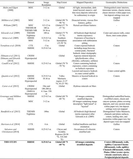
Table 2.1: Summary of Previous Regional and Global Studies ... 37
Table 2.2: Number of Crater Wall Versus Crater Fill/Mound Deposits. ... 38
Figure Captions ... 39
Figure 2.1: Classification scheme ... 43
Figure 2.2: Example crater, canyon, and channel fill and mound deposits ... 44
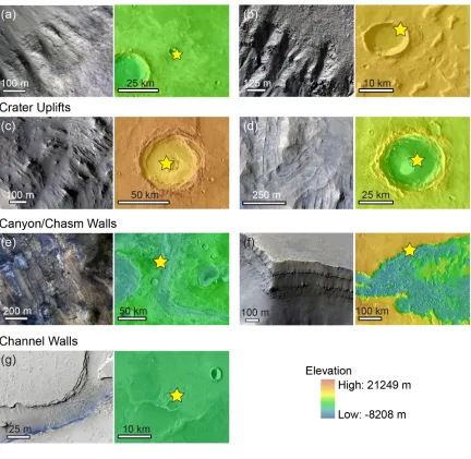
Figure 2.3: Example crater, canyon, and channel wall and uplift deposits ... 45
Figure 2.4: Example intercrater plains deposits ... 46
Figure 2.5: Example “other” deposits ... 47
Figure 2.6: Example glacial/periglacial deposits ... 48
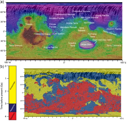
Figure 2.7: Reference maps ... 49
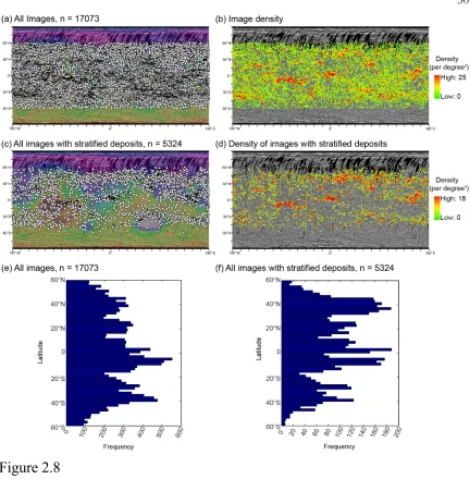
Figure 2.8: Global distributions of HiRISE image database and stratified images ... 50
Figure 2.9: Geomorphic settings of stratified deposits ... 51
Figure 2.10: Mapped distribution of basin fill and unconfined bedrock deposits ... 52
Figure 2.11: Mapped distribution of basin fill and unconfined bedrock deposits by age ... 53
Figure 2.12: Bar plots of basin fill and unconfined bedrock deposits counts ... 54
Figure 2.13: Glacial/periglacial deposits ... 55
Figure 2.14: Map of global depositional processes ... 56
Chapter 3: Page Table 3.1: HiRISE DTMs and Orthoimages ... 105
Table 3.2: Study Sites ... 106
Table 3.3: Basic Bed Thickness Statistics ... 107
Table 3.4: Runs Test Significance Probability Values ... 108
Table 3.5: Lilliefors Probability Significance Values ... 109
Figure Captions ... 110
Figure 3.1: Representative distributions ... 115
Figure 3.2: Global reference map ... 116
Figure 3.3: Geomorphic context of study sites ... 116
Figure 3.4: Holden crater sections ... 117
Figure 3.5: Plateau west of Juventae sections ... 118
Figure 3.6: Gale crater sections ... 118
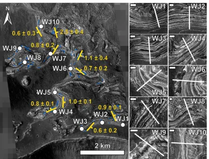
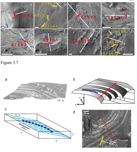
Figure 3.7: Additional sections ... 119
Figure 3.8: Bed orientation measurements ... 119
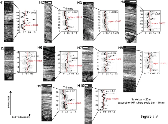
Figure 3.9: Holden bed thickness measurements ... 120
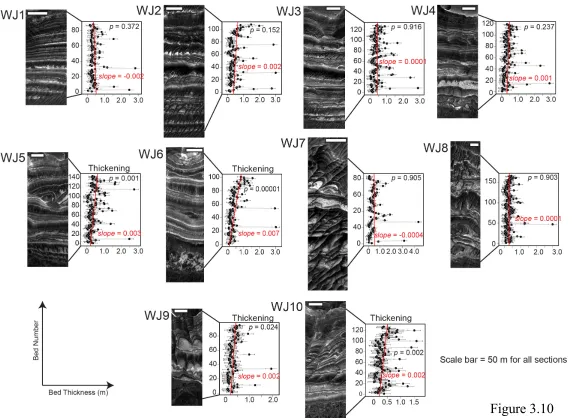
Figure 3.10: Plateau west of Juventae Chasma bed thickness measurements ... 121
Figure 3.11: Gale crater bed thickness measurements ... 122
Figure 3.12: Additional location bed thickness measurements ... 123
Figure 3.13: Histograms ... 124
Figure 3.14: Empirical and theoretical CDF plots ... 125
Figure 3.15: Log-log plots ... 126
Figure 3.16: Stratigraphy of a simple alluvial fan ... 127
x
Chapter 4: Page
Table 4.1: Constrained Model Coefficients ... 170
Table 4.2: Optimized Particle Diameter Ratios ... 171
Table 4.3: Modeled Mass Fractions Using Full Spectrum and Optimized Diameter Ratio ... 172
Table 4.4: Modeled Mass Fractions Using Partial Spectrum and Optimized Diameter Ratio ... 173
Figure Captions ... 174
Figure 4.1: Endmember photomicrographs and histograms ... 179
Figure 4.2: NIR diffuse reflectance spectra of all mixtures and endmembers ... 180
Figure 4.3: Reflectance band minima positions ... 181
Figure 4.4: Reflectance band depths ... 182
Figure 4.5: JCSS-3501 saponite and epsomite measured and modeled mixture spectra ... 183
Figure 4.6: SapCa-2 saponite and epsomite measured and modeled mixture spectra ... 183
Figure 4.7: NAu-2 nontronite and epsomite measured and modeled mixture spectra ... 184
Figure 4.8: SWa-1 nontronite and epsomite measured and modeled mixture spectra ... 184
Figure 4.9: SCa-3 montmorillonite and epsomite measured and modeled mixture spectra ... 185
Figure 4.10: SWy-2 montmorillonite and epsomite measured and modeled mixture spectra ... 185
Figure 4.11: Optimized particle diameter ratios for individual mixtures- full spectra ... 186
Figure 4.12: Modeled vs. measured mass fraction- full spectra, mean particle sizes ... 187
Figure 4.13: Modeled vs. measured mass fraction- full spectra, mode particle sizes ... 188
Figure 4.14: Modeled vs. measured mass fraction- full spectra, optimized particle sizes ... 189
Figure 4.15: Relative uncertainties- full spectra, optimized particle sizes ... 190
Figure 4.16: Optimized particle diameter ratios for individual mixtures- partial spectra ... 191
Figure 4.17: Modeled vs. measured mass fraction- partial spectra, mean particle sizes ... 192
Figure 4.18: Modeled vs. measured mass fraction- partial spectra, mode particle sizes ... 193
Figure 4.19: Modeled vs. measured mass fraction- partial spectra, optimized particle sizes ... 194
Figure 4.20: Relative uncertainties- partial spectra, optimized particle sizes ... 195
Chapter 5: Page Table 5.1: MAHLI Images Used to Measure Size, Shape, and Concentration of Nodules ... 241
Table 5.2: Nodule Size and Shape Statistics ... 242
Table 5.3: Wilcoxon Rank Sum Test Results ... 242
xi
Table 5.5: ChemCam Comparison (wt. %) between Nodule-Rich
vs. Nodule-Free Sheepbed ... 243
Figure Captions ... 244
Figure 5.1: Yellowknife Bay context image and stratigraphic column ... 250
Figure 5.2: MAHLI images of solid, hollow, and filled nodules ... 251
Figure 5.3: MAHLI targets from the Selwyn, John Klein, and Cumberland areas ... 252
Figure 5.4: Size frequency histograms ... 253
Figure 5.5: Plots of hollow nodule rim thickness versus hollow nodule interior void diameter ... 254
Figure 5.6: Navcam overhead projection showing mosaic footprints ... 255
Figure 5.7: Nodule distributions mapped in the John Klein drill site mosaic ... 256
Figure 5.8: Nodule distributions mapped in the Cumberland 1 mosaic ... 257
Figure 5.9: Nodule distributions mapped in the Cumberland 2 mosaic ... 258
Figure 5.10: Nodule distributions mapped in the Raised Ridges and Nodules mosaic ... 259
Figure 5.11: Boundary between upper and lower Sheepbed member ... 260
Figure 5.12: Nodule distributions mapped in the Selwyn mosaic ... 261
Figure 5.13: Nodule distributions mapped in the Yellowknife Bay Egress mosaic ... 262
Figure 5.14: APXS results ... 263
Figure 5.15: ChemCam results ... 264
Figure 5.16: Two models for hollow nodule and filled nodule formation ... 265
Appendix A: Page Table A1: Bed thickness orientation measurements ... 303
Table A2: 1 m orthoimage thinning and thickening results ... 310
Figure A1: Measured section topographic profiles ... 311
xii ACRONYMNS
APXS. Alpha Particle X-Ray Spectrometer
CF. Cumulative Frequency
CFD. Cumulative Frequency Distribution
ChemCam. Chemistry and Camera
CheMin. Chemistry and Mineralogy
CRISM. Compact Reconnaissance Imaging Spectrometer
CTX. Context Camera
DTM. Digital Terrain Model
EP. Expected Precision
FTIR. Fourier Transform Infrared Spectrometer
GIS. Geographic Information System
GLM. Gale Lower Member
GMM. Gale Middle Member
GSD. Ground Sample Distance
GUM. Gale Upper Member
HiRISE. High Resolution Imaging Science Experiment
HRSC. High Resolution Stereo Camera
IR. Infrared
IRB. Infrared Red Blue-green
LIBS. Laser-Induced Breakdown Spectroscopy
xiii Mastcam. Mast Camera
MGS. Mars Global Surveyor
MLE. Maximum Likelihood Estimation
MOC. Mars Orbiter Camera
MOLA. Mars Orbiter Laser Altimeter
MSL. Mars Science Laboratory
Navcam. Navigation Camera
NIR. Near Infrared
OMEGA. Observatoire pour la Minéralogie, l’Eau, les Glaces et l’Activité
PIGWAD. Planetary Interative G.I.S.-on-the-Web Analyzable Database
RAM. Runs Against the Mean
RUD. Runs Up and Down
RMI. Remote Micro-Imager
RSM. Remote Sensing Mast
SAM. Sample Analysis at Mars
TES. Thermal Emission Spectrometer
THEMIS. Thermal Emission Imaging System
USGS. United States Geological Survey
WJ. West of Juventae Chasma
1 C h a p t e r 1
INTRODUCTION
1.1 A Golden Age of Mars Exploration
The past two decades have been a veritable golden age of Mars exploration due to the success of numerous unmanned orbital, landed, and rover missions. Instruments onboard these spacecraft have probed the atmosphere, surface, and interior of Mars, collecting myriad data sets that provide the opportunity to study Mars’ geological history at a level of detail rivaled only by studies of the Earth and Moon. Prior to the phase of increased Mars exploration that began in the mid-1990s, the Mariner and Viking missions provided the first detailed view of the Martian surface. Mariner 9, the first spacecraft to go into orbit around another planet, returned images during the early 1970s of landforms representing a diversity of sedimentary, volcanic, glacial/periglacial, and impact-related processes that had once occurred on the Martian surface [Masursky, 1973]. Launched in 1975 to Utopia Planitia and Chryse Planitia, respectively, the Viking 1 and 2 missions each consisted of an orbiter and a lander. The Viking orbiters took more than 1,400 images of the surface of Mars while the landers carried out environmental and geophysical experiments and provided the first in-situ images of the Martian surface [Soffen, 1976; Arvidson et al., 1989].
2
onboard MGS provided a global view of Mars’ atmosphere, surface, and interior, and included a magnetometer, a gravity field experiment, the Mars Orbiter Camera (MOC), Mars Orbiter Laser Altimeter (MOLA), and the Thermal Emission Spectrometer (TES) [Albee et al., 2001]. Mars Odyssey, a NASA orbiter launched in 2001, consisted of a gamma ray spectrometer, a radiation experiment, and the Thermal Emission Imaging System (THEMIS).
3
exploring Gale crater since August of 2012 [Grotzinger et al., 2012; Grotzinger et al., 2014].
1.2Sedimentary Rock Record of Mars
Images from Mariner 9 first revealed the existence of stratified deposits in the polar and mid-latitude regions of Mars [Murray et al., 1972; Soderblom et al., 1973; Cutts, 1973; Sharp, 1973], and results from the Viking lander [Arvidson et al., 1989] and Pathfinder
[Golombek et al., 1999] suggested the past occurrence of aqueous sedimentary processes. Yet the widespread distribution of sedimentary rocks on Mars was not recognized until the start of the 21st century in a landmark paper by Malin and Edgett [2000]. Malin and Edgett [2000] used high-resolution MOC images onboard MGS to identify and map the distribution of sedimentary rocks on Mars, identifying a record of surface processes spanning several billion years.
Subsequent imaging over the past two decades by HRSC [Neukum et al., 2004], MOC [Malin and Edgett, 2001], CTX, and HiRISE [McEwen et al., 2010; Grotzinger and Milliken, 2012] shows these deposits occurring in diverse settings on Mars that represent
eolian, fluvial, and possibly lacustrine depositional environments [Carr, 1996; Malin and Edgett, 2000; Squyres et al., 2004b; Grotzinger et al., 2011; Grotzinger and Milliken,
4
Gendrin et al., 2005; Bibring et al., 2005, 2006; Mustard et al., 2008; Ehlmann et al., 2008;
Osterloo et al., 2008; Murchie et al., 2009; Carter et al., 2013; Ehlmann and Edwards, 2014]. Recent in situ observations by the Mars Exploration Rovers Spirit and Opportunity [Squyres et al., 2004c; Grotzinger et al., 2005; Squyres et al., 2007; Arvidson et al., 2014] and by the Mars Science Laboratory Curiosity rover [Williams et al., 2013; Vaniman et al., 2014; McLennan et al., 2014; Ming et al., 2014; Grotzinger et al., 2014] have enabled outcrop-scale geological investigations of sedimentary rock record.
1.3Dissertation Summary
With the advent of high resolution orbital and rover investigations of Mars described above, the study of Mars’ sedimentary rock record can transition from an exploratory phase based primarily on qualitative observations to one in which quantitative analyses provide constraints on the evolution of depositional and diagenetic environments on Mars. The following chapters will illustrate how the synthesis of global data sets and the application of statistical methods to orbital, rover, and laboratory data can be used to advance our understanding of the Martian rock record.
5
limitations of orbital data sets. This study explores ways in which orbital bed thickness measurements can provide an objective and quantitative approach for describing the depositional history of Martian stratified deposits. Chapter 4 presents a study of laboratory spectra of fine-grained mixtures of clay and sulfate minerals. This study assesses the ability of spectral mixing models to reproduce spectra of these mixtures and derive mineral abundances from mixture spectra. This study was undertaken in the laboratory, but its results are broadly applicable to the detection and quantification of hydrated minerals in sedimentary deposits on Mars. Chapter 5 presents a quantitative analysis of the size, shape, and spatial distribution of diagenetic nodules observed by the MSL Curiosity rover in Gale crater. Understanding the origin and distribution of nodules in the Sheepbed member is essential to reconstructing the diagenetic aqueous history of the Yellowknife Bay formation and assessing its potential habitability.
1.4Data and Methods
1.4.1 Spacecraft Instrument Data
Data from the instruments described below are used in this dissertation.
1.4.1.1 Mars Orbiter Laser Altimeter (MOLA)
6
The altitude of the surface was measured by calculating the time elapsed between pulse emission from the instrument and signal return to the spacecraft’s collection mirror after reflecting off the surface of Mars.
A MOLA topographic map created by Goddard Spaceflight Center at a resolution of 128 pixels per degree was used in Chapter 2 to identify the geomorphic setting of each stratified deposit identified in HiRISE images. This MOLA map was also used in Chapters 3 and 5 as a basemap for displaying the topographic setting of study sites. This map is available for download online at http://webgis.wr.usgs.gov, the United States Geological Survey (USGS) Planetary Interactive G.I.S.-on-the-Web Analyzable Database (PIGWAD).
1.4.1.2 Thermal Emission Imaging System (THEMIS)
7
1.4.1.3 High Resolution Imaging Science Experiment (HiRISE)
The HiRISE camera onboard MRO is a three-mirror astigmatic reflecting telescope with a Cassegrain objective. Launched in 2005, HiRISE took its first image of the Martian surface in September 2006 at the highest level of detail ever achieved by an orbital camera. HiRISE images the surface of Mars at resolutions between 0.25-1.3 meters per pixel in red (panchromatic), blue-green (BG), and near infrared (NIR) wavelength bands, and can resolve objects on the order of 1 meter due to the high resolution and high signal-to-noise ratio achieved by the camera [McEwen et al., 2007]. Since 2006, HiRISE has acquired nearly 30,000 images covering about 2% of the Martian surface.1 HiRISE images of the same area on the surface taken at different look angles (stereo-pairs) can be used to make Digital Terrain Models (DTMs) with a post-spacing of 1-2 meters and vertical precision of tens of centimeters [Kirk et al., 2008].
HiRISE images are used in Chapter 2 to identify and classify stratified deposits. In Chapter 3, HiRISE orthoimages and DTMs are used to measure bed thickness in stratified deposits. A HiRISE image is also used in Chapter 5 to display the location of MSL Curiosity rover targets. All HiRISE images used in this dissertation are available for download online from the Planetary Data System (PDS) at https://pds.jpl.nasa.gov or from the HiRISE website at http://hirise.lpl.arizona.edu. HiRISE DTMs used in this study are available for download from the HiRISE website at http://hirise.lpl.arizona.edu/dtm.
1 Recent image coverage statistics were stated in a Smithsonian.com article by Magan Gambino titled, “This is Mars in
8
1.4.1.4 Mars Science Laboratory (MSL) Curiosity Rover
The MSL mission to Gale crater launched in November of 2011 and successfully delivered the Curiosity rover to the surface of Mars in August of 2012. The payload of the Curiosity rover consists of a sophisticated suite of cameras, spectrometers, radiation detectors, and environmental and atmospheric sensors. Chapter 5 of this thesis presents new analysis of data from Mast Camera (Mastcam), Mars Hand Lens Imager (MAHLI), Alpha Particle X-Ray Spectrometer (APXS), and Chemistry and Camera (ChemCam) instrument, and uses images from the Navigation camera (Navcam) as a basemap. K. Stack performed the analysis of Mastcam and MAHLI data presented in Chapter 5; the APXS analysis was contributed by M. Schmidt and R. Lee and the ChemCam analysis was contributed by N. Mangold and M. Nachon. K. Stack synthesized the results from all instruments.
9
1.3-7 meters away from the rover mast [Maurice et al., 2012; Wiens et al., 2012]. The ChemCam laser has a spot size 0.35-0.55 millimeters in diameter and produces a plasma when interacting with a surface sample. The photon emission from this plasma can be used to detect major, minor, and trace elements with the ChemCam spectrometers. ChemCam also includes a Remote Micro-Imager (RMI) to provide context images with a 20 milliradian field of view and submillimeter pixel resolution.
Curiosity’s MAHLI camera and APXS are mounted on the rover arm. MAHLI is a 2-megapixel focusable camera capable of imaging objects at working distances between 2.1 centimeters and infinity at a maximum resolution of ~14 micrometers [Edgett et al., 2012]. At the minimum working distance, a MAHLI pixel is 14 by 14 micrometers and a full image measures 1600 by 1200 pixels. The APXS is mounted on the rover arm and uses a combination of X-ray fluorescence and particle-induced X-ray emission to measure the bulk chemical composition of rocks and soils [Campbell et al., 2012].
1.4.2 Software
The data analysis presented in this dissertation was performed primarily with ArcGIS and MATLAB software packages. Excel, Adobe Illustrator, and ENVI were also used.
1.4.2.1 ArcGIS
10
distribution of nodules in rover images. The global stratified deposit database and geologic map shapefiles presented in Chapter 2 were plotted in ArcGIS on MOLA and THEMIS Mars 2000 equicylindrical projected basemaps. In Chapter 3, X, Y, and Z coordinates were extracted from HiRISE orthoimages and DTMs in ArcGIS to calculate bed orientation and bed thickness. In Chapter 5, the distribution and size of diagenetic nodules were mapped using Mastcam and MAHLI images loaded into ArcGIS. Spatial analyst tools provided in the software package were used to calculate the size and statistical distribution of the different nodule types.
1.4.2.2 MATLAB
All data plots (excluding maps produced in ArcGIS) presented in Chapters 3, 4, and 5 were created using MATLAB scripts written by K. Stack. The orientation of bedding planes measured in HiRISE images in Chapter 3 were calculated using a MATLAB script written by J. Metz [Metz, 2010] and modified by K. Stack and A. Hayes. Spectral unmixing was performed in Chapter 4 using a code written by R. Milliken and modified by K. Stack.
1.4.3 Laboratory Instruments
1.4.3.1 Fourier Transform Infrared Spectrometer (FTIR)
11
12 C h a p t e r 2
GLOBAL DISTRIBUTION OF STRATIFIED ROCKS ON MARS
Abstract
13
stratigraphic correlations essential for refining and globally correlating a Martian geologic time scale.
2.1 Introduction
Stratification within the rock record represents a time series of depositional and erosional events in which rock volumes are bounded by surfaces of erosion or nondeposition [Blackwelder and Barrows, 1911; Wheeler, 1958, 1959; Sloss, 1963; Sadler, 1981; Christie-Blick and Driscoll, 1995]. Changes within these time series, whether related to the chemical, biological, or physical properties of the rocks, provide important insight into the evolution of depositional environments and processes on both local and global scales. The wealth of information recorded in stratified rocks also enables the correlation of spatially distinct deposits, a critical step in the development of a planet’s geologic time scale [McLennan and Grotzinger, 2008; Grotzinger et al., 2011; Grotzinger and Milliken, 2012].
14
and deposition through time, that are related to past climate, aqueous processes, and habitability of the Martian surface.
The widespread coverage of high-resolution images of the Martian surface now provides an opportunity to study the rock record of Mars at an unprecedented level of detail. Mariner 9 images returned during the early 1970s first revealed the existence of stratified deposits in the polar and mid-latitude regions of Mars, e.g. Cutts [1973], Sharp [1973]. It was nearly thirty more years before the widespread occurrence and global importance of sedimentary rocks on Mars was recognized by Malin and Edgett [2000] as a result of the high-resolution global imaging campaign of the Mars Global Surveyor (MGS) Mars Orbiter Camera (MOC) [Malin and Edgett, 2001]. Subsequent imaging over the past two decades has led to the discovery of a diversity of past surface processes, and images from MOC, High Resolution Stereo Camera (HRSC) [Neukum et al., 2004], Context Imager (CTX), the High Resolution Imaging Science Experiment (HiRISE) [McEwen et al., 2007], and in situ studies by rovers and landers [Squyres et al., 2004a; Grotzinger et al.,
2005; Jaumann et al., 2007; Grotzinger et al., 2014] have provided abundant evidence for a myriad of past volcanic, impact, glacial/periglacial, and sedimentary processes occurring at the Martian surface.
15
specific feature or class of features, i.e., Williams [2007] and Caudill et al. [2012]. Other studies employ the highest resolution image data available, but are focused on particular regions of Mars, i.e., Quantin et al. [2012] and Salvatore and Christiansen [2014]. Using an inventory of HiRISE images, Grotzinger and Milliken [2012] presented a global synthesis of inferred sedimentary deposits, and suggested an initial approach of recognizing “orbital facies,” defined by a limited range of distinctive attributes inherent to the strata themselves (Table 2.1). However, the Grotzinger and Milliken [2012] inventory goes no further than identifying several “type sections” representing each orbital facies. The global distribution and significance of each orbital facies is largely unknown. Applying the exact orbital facies of Grotzinger and Milliken [2012] on a global scale is difficult because analysis of VNIR spectral data is needed to identify several of their orbital facies, but the widespread classification of stratified rocks by geomorphic and depositional setting and terrain age is possible given the global coverage of high resolution topographic and image data sets.
Building specifically on the work of Malin and Edgett [2000] and Grotzinger and Milliken [2012], this study presents a comprehensive inventory of Martian stratified
16 2.2 Data and Methods
2.2.1 Data
The HiRISE camera on-board the Mars Reconnaissance Orbiter (MRO) is a three-mirror astigmatic reflecting telescope with a Cassegrain objective that images the surface of Mars at scales between 0.25-1.3 meters per pixel [McEwen et al., 2007]. HiRISE has three filters: red (panchromatic), blue-green (BG), and near infrared (NIR) wavelength bands, and can resolve objects on the order of 1 meter due to the high resolution and high signal-to-noise ratio achieved by the camera. Launched in 2005, MRO entered into Mars orbit in March of 2006, and HiRISE took its first image of the Martian surface in September 2006 at the highest level of detail ever achieved by an orbital camera. Since 2006, HiRISE has acquired nearly 30,000 images covering about 2% of the Martian surface.2
The HiRISE image database used in this study contains 17,073 HiRISE images acquired between September 2006-January 1, 2013 within the latitude range of 60 degrees north and south of the Martian equator. The polar and high latitude regions of Mars were excluded from this study because of the predominance of ice-related surface ‘mantling’ deposits and periglacial features in these regions of Mars that largely obscure bedrock outcrops [Milliken et al., 2003; Head et al., 2003; Edwards et al., 2009]. The list of HiRISE images used here was obtained from the Planetary Data System (https://pds.jpl.nasa.gov) and organized according to latitude and longitude. Calibration images, dust-obscured images, and duplicate images, i.e., second image acquired as part of a stereo-pair or subsequent images identified explicitly by the HiRISE team as part of change detection
2 Recent image coverage statistics were stated in a Smithsonian.com article by Magan Gambino titled, “This is Mars in
17
monitoring campaigns, were excluded from the database. Not all duplicate images are listed as stereo pairs or change detection images, so some repeat images are present in the database, although an attempt was made to remove them when found. All HiRISE images in the database were viewed at full-resolution using links from the HiRISE website (http://hirise.lpl.arizona.edu), and the HiView application.
2.2.2 Image classification
18
Deposits were also classified by setting within each broad geomorphic category (Figure 2.1). Basin fill deposits are those that appear to be topographically confined and include fills and mounds found within craters, canyons, chasms, and channels. Deposits that do not appear to be controlled by modern-day topography at the length-scale of individual crater or canyon basins are categorized as unconfined stratified rock and include wall and uplift deposits, plains deposits, and most examples within the “other” category. A designation of unconfined stratified rock does not mean that the deposits were never controlled by topography, rather it means that it is not possible to define this topographic control today. Also identified within the database are those stratified deposits suspected of being periglacial in origin due to the association of these deposits with dissected mantle terrain, i.e., Mustard et al. [2001] and Milliken et al. [2003], or the occurrence these deposits as concentric craters fills, lobate debris aprons, or lineated valley fills, e.g., Squyres and Carr [1986] and Carr [2001]. These deposits represent only those showing
clear stratification in existing HiRISE coverage and are not meant to represent a comprehensive survey of all periglacial and viscous flow features on Mars, e.g., Souness et al. [2012].
19
times, once for each occurance of a stratified rock exposure. These duplicate images are not counted towards the total number of images listed above, or presented in Figure 2.8.
2.2.3 Spatial Analysis
All images in the database (Figure 2.8a) and all images in the database containing stratified deposits (Figure 2.8c) were plotted on a THEMIS Day IR equicylindrical projection basemap as single points according to the center latitude and longtitude of each image. Histograms (Figure 2.8e and 2.8f) and point densities (Figure 2.8b and 2.8d) were calculated from the database using the ArcGIS Spatial Analyst toolbox to assess the distribution of images and images containing stratified deposits across the surface of Mars, and to illustrate potential spatial sampling biases that may be inherent to the data set. Point densities were calculated in units of square degrees using a circular area around each point with a defined radius and map cell size of 1 degree.
In order to examine the distribution and setting of stratified deposits in terrains of different ages, the locations of identified stratified deposits were overlain on a geologic map of Noachian, Hesperian, and Amazonian-aged terrains compiled from Mars Global Geologic Map 1802ABC [Scott and Tanaka, 1986; Tanaka and Scott, 1987; Greeley and Guest, 1987] (Figure 2.7). The stratified deposit database was also grouped by geomorphic
20 2.3 Results
2.3.1 Global Distribution of Stratified Deposits
Of the 17,073 HiRISE images examined in this study, 5,324 contain stratified rock in one or more geomorphic setting or deposit type (Figure 2.8). Counting images that have been double book-kept for the presence of stratified deposits in one or more settings, there are 5,781 unique stratified deposits observed in the HiRISE image inventory. Figures 2.8c and 2.8f show that stratified deposits occur ubiquitously throughout the latitude range from 60º N to 60º S, and are widespread over all longitudes. The histogram in Figure 2.8f shows a slight overall decrease in the number of images containing stratified deposits moving from the northern to southern hemispheres, but besides this weak trend there appears to be no clear latitudinal control on the distribution of stratified deposits that could not also be partially explained by the overall image distribution (Figure 2.8e), as described below.
30-21
40º S range, which includes images of stratified material in southern Terra Cimmeria and Terra Sirenum. In contrast, there is a disproportionate number of images in the 30-45º N range that contain stratified deposits relative to the overall number of images taken in this region. This suggests that the high concentration of images containing stratified deposits in the Deuteronilus, Protonilus, and Nilo Syrtis Mensae regions truly represents an abundance of stratified deposits present in this area that is not simply a reflection of an image acquisition bias in this area. Areas with a relatively low density of images containing stratified deposits include northern Terra Cimmeria and eastern Tyrrhena Terra, Terra Sabaea, and northern Noachis Terra.
2.3.2 Geomorphic Setting of Stratified Deposits
22
deposits. Stratified plains deposits also occur throughout Elysium Planitia and the Tharsis region.
Canyon deposits are largely concentrated near the equator in Valles Marineris and in the northern hemisphere, particularly along the dichotomy boundary between the southern highlands and northern lowlands. Aside from areas of high density, canyon deposits are also observed to be fairly widespread throughout the Elysium Planitia and Tharsis regions, where layered lavas flows are frequently exposed in fissure and catena walls, both landforms tabulated in the canyon/chasm category. Aside from deposits north of Argyre Planitia, in the Uzboi-Margaritifer-Ladon system, and Niger and Dao Vallis in eastern Hellas Basin, canyon/chasm deposits are sparse below ~15º S. The “other” category of deposits, which includes volcanic constructs, crater ejecta, and odd features like the Acidalia mounds, are also largely limited to the northern lowlands.
23
Noachian-aged terrains such as Meridiani Planum and in the plains north of Hellas basin. Very few of the “other” category of deposits are found in Noachian-age terrains, instead occurring nearly equally in terrains of Hesperian of Amazonian age. Again, this is not unexpected, as this category consists largely of volcanic constructs of Hesperian or Amazonian age and deposits associated with well-defined crater ejecta at the modern surface, where the latter is not likely to be preserved due to erosion for older Noachian craters.
2.3.3 Basin Fill versus Unconfined Stratified Deposits
24
and only 22% are found in Amazonian-aged terrains. In contrast, the percentage of unconfined stratified deposits, which consists predominantly of crater, canyon, and channel wall deposits, found in Noachian (30%), Hesperian (35%), and Amazonian (35%) terrains remains fairly constant (Figure 2.12a). The successive decrease in the proportion of basin fill deposits in younger terrains is also illustrated in Figure 2.12b, in which Noachian-aged terrains contain 40% basin fill deposits and 60% unconfined stratified deposits, while Amazonian terrains contain only 23% basin fill deposits and 77% unconfined stratified deposits.
2.3.4 Glacial/Periglacial Deposits
25 2.4 Discussion
2.4.1 Global Distribution and Comparison to Previous Studies
The widespread occurrence of stratified deposits over the surface of Mars in terrains of all ages implies the preservation of a time series of discrete depositional events spanning nearly 4 billion years from the Noachian to Amazonian periods. The database compiled here shows that the stratified rock record of Mars is more extensively exposed than indicated by previous studies [Malin and Edgett, 2000; Edwards et al., 2009; Grotzinger and Milliken, 2012] that took a similar global-scale approach. Edwards et al.
26
geological processes operating during early Martian history is preserved in the rock record, although the degree to which the observed strata simply represent impact-related processes remains unclear.
The global distribution of stratified deposits inventoried here is also much more widespread than that presented in Malin and Edgett [2000], although that mapping effort included only those deposits inferred to be sedimentary in origin based on criteria including induration, apparent fine grain-size, and the presence of repetitive bedding. Definitively quantifying grain-size is impossible even at the resolution of HiRISE, and repetitive bedding is difficult to define for thin deposits like those found in crater or canyon wall deposits. As a result, these distinctions were not made in this study’s database, so the deposits identified herein include stratified deposits of sedimentary but also likely volcanic, glacial/periglacial, and impact origin. Additional work at a level of detail beyond the scope of this global database is likely needed to definitively distinguish sedimentary, volcanic, glacial/periglacial, or impact processes.
This study also finds stratified deposits to be more extensive than that of Grotzinger and Millken [2012], who examined a smaller subset (~1/3) of the images included in the
database presented here. Grotzinger and Milliken [2012] noted a concentration of stratified deposits near equatorial regions that is not observed in this larger database. The distribution of stratified deposits observed at higher latitudes observed in this study is more consistent with the identification of stratified deposits in high latitude regions also recognized by Schon et al. [2009]. Discrepancies between this study’s database and that of Grotzinger and
27
different criteria used to identify stratified deposits. Given the large number of images examined in the present study and their near-global distribution, the results presented here are a more accurate representation of the true global distribution of stratified deposits on Mars than previous studies based on more limited datasets.
2.4.2 Implications for the Martian Sediment and Hydrological Cycles
The inventory of basin fill versus unconfined stratified deposits presented in Figures 2.10-2.12 indicates basin filling materials are more commonly associated with the oldest Noachian-aged terrains relative to younger, Amazonian terrains in which unconfined stratified deposits are most prevalent. The following discussion will explore possible explanations for this observed trend, but first an important aspect of relative age dating on the surface of Mars must be considered.
Because in-situ absolute age dating techniques are not currently developed for widespread application on the surface of Mars, relative crater dating techniques [Hartmann and Neukum, 2001] are still the primary method of relative age dating on Mars. These
28
deposits found within the craters of that surface. Therefore, basin-filling deposits observed in Noachian-aged terrains can only be robustly described as Noachian-aged or younger, while similar deposits found in Hesperian-aged terrains can only be constrained as Hesperian-aged or younger, unless specific cross-cutting relationships with other deposits of known relative age are observed or smaller-scale crater counts are attempted.
29
there is an apparent bias of crater-filling deposits in higher elevation Noachian terrains. Therefore, the decreased availability of topographic basins in younger terrains on Mars is not a likely explanation for the skew of basin-filling deposits towards older terrains.
Alternatively, if the age of the basin-filling deposits is comparable to the age of the terrains in which they are located, the predominance of stratified basin-filling deposits in older terrains with successively fewer basin-filling deposits in Hesperian and Amazonian terrains, could be broadly representative of global-scale changes in the sediment cycle through time. Grotzinger et al. [2011] and Grotzinger and Milliken [2012] presented a conceptual model in which volcanic activity and the higher rate of impact cratering early in Mars’ history resulted in an increased flux of sediment. In this model, a more active cycle of sediment production, erosion, and deposition during the Noachian and early Hesperian could have led to the fairly widespread deposition of stratified sedimentary deposits in the oldest craters and canyons. Golombek and Bridges [2000] and Golombek et al. [2006] also suggested a decrease in the Martian sediment cycle, using data from the Pathfinder and Mars Exploration Rover landing sites extrapolated to the entire planet to show a 4-6 fold decrease in erosion rates during the Hesperian and Amazonian periods compared to the late Noachian/early Hesperian. These studies proposed a largely conceptual model. The skew of basin fill deposits in older terrains observed in this study’s global dataset can support this conceptual model with observations.
30
widespread lithification and cementation of basin-filling sedimentary deposits, i.e., Andrews-Hanna et al. [2010]. The transition to arid conditions during the Late Noachian
[Andrews-Hanna and Lewis, 2011] associated with the loss of water and a deepening of the water table would have prevented the widespread preservation of stratified sedimentary deposits in younger terrains on Mars even if the sedimentary cycle had remained active into the Amazonian.
2.4.3 Global-Scale Depositional Processes on Mars
Conclusively distinguishing between sedimentary, volcanic, glacial/periglacial, and impact origins for Martian stratified deposits requires detailed observations at a scale not possible in even the highest resolution orbital images available. Making these distinctions can be challenging even with in situ observations from sophisticated rover payloads [Grotzinger et al., 2014]. In many cases, a synthesis of orbital and rover observations and geochemical and image data is needed to reconstruct the depositional history of a sequence of rocks. Yet one of the major reasons for creating a comprehensive inventory of stratified deposits was to gain insight into the processes responsible for the deposition of the Martian rock record. Examining the distribution of stratified deposits in specific geomorphic settings with respect to major volcanic centers, predicted pyroclastic deposits, and regions where glacial/periglacial processes occur (Figure 2.14), can provide some basic constraints on the relative importance of these processes in the development of Mars’ rock record.
31
depositional processes operating on planet-wide scales. The location of major volcanic centers relative to the global distribution of stratified deposits (Figure 2.14) suggests that many of the stratified deposits in Amazonian-aged terrains, particularly those in the vicinity of these volcanic centers, can be explained by effusive lava flows. Examples of stratified lavas can be found in the global database, particularly in the layered scarps and flanks of the major Martian volcanoes, stratified lobes of lavas in plains in the Tharsis region and Elysium Planitia, and in the stratigraphy preserved in the walls of catenas, pit craters, and fissures in close proximity to these major volcanic centers (Figure 2.14). These findings are consistent with those of Bandfield et al. [2013], who find a predominance of blocky effusive lavas in younger, Amazonian-aged terrains. Pyroclastic volcanism, as proposed by Kerber et al. [2012] and Bandfield et al. [2013], may be more effective at widespread distribution of material over the surface of Mars. Isopach maps of predicted pyroclastic deposit thickness produced by Kerber et al. [2012] plotted together with this study’s stratified deposit database (Figure 2.14) show that many stratified deposits fit within the predicted regions of thick pyroclastic deposition. Approximately 3000 stratified deposits are located in regions near major volcanic centers and in areas of predicted thick pyroclastic deposition (Figure 2.14), suggesting that ~50% of all observed stratified deposits could be reasonably explained by extrusive volcanic processes. However, as Kerber et al. noted and can be seen in Figure 2.14, models of pyroclastic accumulation and
32
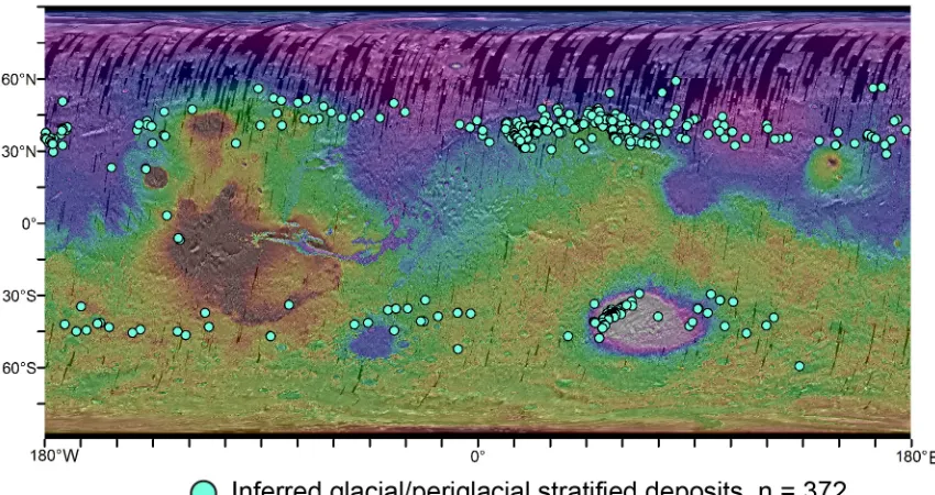
Glacial/periglacial processes can partially explain the distribution of stratified deposits, particularly at latitude ranges greater than 30º N and S, where these processes are known to occur [Milliken et al., 2003; Head et al., 2003; Schon et al., 2009]. Approximately 400 basin fill and intercrater plains deposits observed in the database are associated with glacial/periglacial features, but nearly half (43%) of the entire inventory of 5,777 stratified deposits is located between 30-60° N or S in regions known to host numerous glacier-like forms [Souness et al., 2012]. Of course not all of the deposits observed in these latitude ranges exhibit evidence for glacial processes, but the predominance of stratified deposits in these regions suggests that low temperature processes are important, and perhaps underappreciated, contributors to the stratified rock record of Mars.
33
examples presented in Figure 2.2a-2.2h and Figure 2.6, and are most likely formed by sedimentary, glacial/periglacial, or volcaniclastic processes. In addition approximately half of all observed intercrater plains (~700 deposits) and wall/uplift deposits (~1000) are located in regions with no nearby volcanic centers, where predicted pyroclastic accumulation is fairly low (Figure 2.14). The basin fill deposits together with the intercrater plains and wall/uplift deposits not located near major volcanic centers make up ~50% of the deposits observed in this study, and represent an initial estimate for the contribution of sedimentary processes, although the ~400 deposits of glacial/periglacial origin are also included in this value. As mentioned above, in situ observations are likely needed to make more conclusive process-based distinctions. Still, the widespread occurrence of basin-fill deposits, particularly in the oldest terrains of Mars, where predicted pyroclastic accumulations are low and evidence for glacial/periglacial processes is sparse, requires the likely widespread occurrence of eolian, fluvial, and/or lacustrine sedimentary processes.
34
In the absence of widely applicable absolute age dating techniques on Mars, high-resolution image data sets and spectral observations become the primary tools for correlating spatially distinct deposits. However, on a largely basaltic planet such as Mars, mineral assemblages need not uniquely reflect one particular depositional process or time period, and may only be applicable for stratigraphic correlations in the most general sense, i.e., Bibring et al., [2006]. The global distribution of stratified deposits presented here can aid in identifying regions on Mars where orbital stratigraphic correlations may be most successful. For example, high-density areas of unconfined stratified deposits in terrains of similar age may allow successful correlations between spatially distinct crater and canyon wall deposits. Good candidates for this type of future analysis include Noachian-aged terrains in Terra Cimmeria, Terra Sirenum, Meridiani Planum, and Western Arabia Terra, Hesperian deposits in Valles Marineris, and Amazonian-aged terrains in Elysium, Utopia, and Deuteronilus Mensae.
35 2.5 Conclusions
This study presents the most comprehensive and highest resolution database of stratified deposits yet compiled for Mars. This database shows that:
(1) Stratified deposits occur globally on Mars throughout terrains of Noachian, Hesperian, and Amazonian age.
(2) Stratified deposits are found most commonly in craters, but canyons/chasms, channels, and plains provide additional geomorphic settings in which stratified deposits occur.
(3) Unconfined stratified deposits (crater walls, uplifts, plains deposits) occur ubiquitously on the surface of Mars and generally outnumber basin-filling deposits.
(4) Basin-filling materials are slightly skewed towards Noachian-aged terrains. This trend is consistent with decreased activity of the sedimentary cycle over time, or a bias towards preservation of older basin-filling deposits.
36
37 TABLES
Table 2.1. Summary of Previous Regional and Global Studies
Dataset Image
Resolution Map Extent Mapped Deposit(s) Geomorphic Distinctions
Malin and Edgett
[2000] MOC 3-12 m Global All light, intermediate, dark-toned layered, massive, and thin mesa deposits inferred to
be sedimentary in origin
Distinguished crater interiors, intercrater terrain, chaotic terrain, chasm interiors within paper text, but deposit settings were not
mapped
Milliken et al. [2003] MOC 3-12 m Global (90 °N -90 °S)
Dissected terrain, viscous flow features, gullies
Gullies
Williams [2007] MOC 0.5-12 m Global (57 °N -57 °S)
Raised curvilinear features - THEMIS IR 100 m
THEMIS NIR 18-36 m
Edwards et al. [2009] THEMIS
Nighttime 100 m Global (75 °N -75 °S) All bedrock (high thermal inertia exposures) Crater and canyon walls, crater floors, inter-crater plains
Schon et al. (2009) HiRISE 0.25-0.5 m Southern hemisphere
(25-50 °S)
Exposures of layering in association with sublimation
pitting
- MOC 3-12 m
Tornabene et al. (2010) CTX ~5 m Global Crater-exposed bedrock including mega breccias; central peaks; fractured bedrock; intact stratigraphy
Craters HiRISE 0.25-0.5 m
Ehlmann et al. [2011];
Ehlmann and Edwards
[2014]
CRISM Hyperspectral
Global Aqueous mineral deposits (phyllosilicates, silica, chlorides, carbonates, sulfates)
-
Caudill et al. [2012] HiRISE 0.25-0.5 m Global (70 °N
-70 °S) exposures; craters containing Craters containing bedrock no bedrock exposures
Craters
Layered and massive bedrock
in crater central uplifts Crater central uplifts
Quantin et al. [2012] HiRISE 0.25-0.5 m Valles Marineris region (3-37 °N, 93-25 °W)
Massive or layered bedrock in
craters Craters
CRISM
Hyperspectral 18-36 m
Carter et al. [2013] CRISM
Hyperspectral 100-200 m 18m and Global Hydrous minerals on Mars OMEGA
Hyperspectral 4.1 km- 350 m
Grotzinger and Milliken
[2012] HiRISE 0.25-0.5 m Global (60 °N -60 °S) All images containing stratified deposits Distinguished underfilled basins, overfilled craters, chasm and canyon systems, plains covering deposits, and very ancient strata within paper text, but deposit
settings were not mapped MOC 3-12 m All images containing image
description "light-toned" or "layered"
Bandfield et al. [2013] THEMIS
Nighttime 100m Global All bedrock (high thermal inertia exposures) after Edwards et al. (2009)
Distinguished Valles Marineris, channels and plains surfaces,
craters, landing sites, and meteorites within paper text, but
deposit types were not mapped
Harrison et al. [2014] CTX 6 m Global Gullied landforms and their
orientation Gullies
Salvatore and
Christiansen [2014] HiRISE 0.25-0.5 m Chryse and Acidalia Regions (20-50
°N, 310-360 °E)
Occurrences of a discrete
stratified unit Craters
THIS STUDY HiRISE 0.25-0.5 m Global (60 °N
-60 °S) All images containing stratified deposits Craters (fill/mounds, walls, uplifts); Canyons/Chasms (fill/mounds, walls, uplifts); Channels (fill/mounds, walls);
38 Table 2.2. Number of Crater Wall versus Crater Fill/Mound Deposits
# of Images Containing:
Terrain Age
Crater Walls
Crater Fills/Mounds
Amazonian 408 213
Hesperian 535 354
39 FIGURE CAPTIONS
Figure 2.1. Classification scheme applied to each image in the dataset.
Figure 2.2. Example basin fill deposits found in craters, canyons, and channels in HiRISE IRB color images (left) located on MOLA topography (right). (a) Terby crater, PSP_002216_1525, (b) Danielson crater, ESP_026626_1885, (c) Eberwalde crater, PSP_001336_1560, (d) Cross crater, ESP_016175_1495, (e) Ius Chasma, ESP_021552_1725, (f) Juventae Chasma, ESP_016712_1760, (g) Melas Chasma, ESP_012638_1700, (h) Nilo Syrtis Mensae, ESP_028509_2140, (i) Athabasca Vallis, ESP_027042_1895, (j) Shalbatana Vallis, ESP_030135_1830.
Figure 2.3. Crater, canyon/chasm, and channel wall and uplift deposits. HiRISE IRB color (left), MOLA topography (right). (a) Crater in Tempe Terra, ESP_012611_2170, (b) Unknown crater, ESP_016163_1395, (c) Martin crater, ESP_011952_1585, (d) Crater in Lunae Planum, ESP_017833_1975, (e) Mawrth Vallis, ESP_018530_2045, (f) Capri Chasma, ESP_018017_1680, (g) Lethe Vallis, PSP_007553_1845.
40
Figure 2.5. Examples of volcanic constructs, crater ejecta, and miscellaneous other deposits. HIRISE IRB color image (left), MOLA topography (right). (a) Ceraunius Catena, PSP_007022_2175, (b) Olympus Mons scarp, ESP_013998_2035, (c) Olympus Mons caldera, PSP_007669_1980, (d) Ascraeus Mons caldera, ESP_026313_1910, (e) Layered ejecta of Kontum crater, ESP_028435_1480, (f) Layered ejecta of Toro crater, ESP_029867_1980, (g) Mound in Xanthe Dorsa, ESP_025822_2165.
Figure 2.6. Examples of glacial/periglacial deposits. HiRISE IRB color (left), MOLA topography (right). (a) Concentric crater fill in unknown crater, PSP_007022_2175, (b) Swirly layers in Hellas basin, ESP_025635_1395, (c) Valley fill in Mamers Vallis, ESP_013254_2115.
Figure 2.7. (a) MOLA elevation draped on THEMIS Day IR showing place names mentioned in this chapter. (b) Timescale showing approximate ages of Noachian, Hesperian, and Amazonian periods and geologic map of Noachian, Hesperian, and Amazonian aged terrains from Mars Global Geologic Map 1802ABC [Scott and Tanaka, 1986; Tanaka and Scott, 1987; Greeley and Guest, 1987].
41
this map and the map in (b). (e) Latitude histogram plotted for all images in the database. (f) Latitude histogram plotted for all images containing stratified deposits.
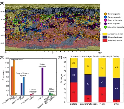
Figure 2.9. (a) Images containing stratified deposits, color coded by geomorphic setting plotted on geologic map of Noachian, Hesperian, and Amazonian-aged terrains. (b) Histogram showing the number of images containing deposits in craters, canyon/chasms, channels, plains, and other. (c) Bar graph showing the percent of images within each geomorphic setting category within Noachian, Hesperian, and Amazonian terrains. Note that canyons/chasms and channels have been counted together in this graph.
Figure 2.10. (a) All unconfined stratified deposits plotted on geologic map of Noachian, Hesperian, and Amazonian-aged terrains. (b) All basin fill deposits. (c) Basin fill and unconfined stratified deposits plotted together.
42
Figure 2.12. (a) Bar graph showing the percent of images located in Noachian, Hesperian, or Amazonian aged terrains, grouped by setting type (basin fill or unconfined stratified deposits). (c) Bar graph showing percent of images that contain unconfined stratified or basin fill deposits, grouped by terrain age.
Figure 2.13. Distribution of images containing stratified deposits associated with glacial/periglacial landforms.
43
44
45
46
47
48
49
50
51
52
53
54
55
56
57 C h a p t e r 3
BED THICKNESS DISTRIBUTIONS ON MARS: AN ORBITAL PERSPECTIVE
Originally published in:
Stack, K. M., J. P. Grotzinger, and R. E. Milliken (2013), Bed thickness distributions on Mars: An orbital perspective, Journal of Geophysical Research- Planets, 118, 1-27, doi:10.1002/jgre.20092.
Abstract
58
sedimentary rocks on Mars. In particular, bed thickness statistics are particularly well suited for examining changes in sediment supply and accommodation within Martian sedimentary sequences.
3.1 Introduction
In situ and remote observations of the Martian sedimentary record have shown that bedding is as fundamental a characteristic of sedimentary rocks on Mars as it is on Earth [Malin and Edgett, 2000; Grotzinger and Milliken, 2012]. Where primary, bedding generally represents a profound attribute of the stratigraphic record: the presence of hiatuses where time is represented by a surface rather than a volume of rock [Blackwelder and Barrows, 1911; Wheeler, 1958, 1959; Sloss, 1963; Sadler, 1981; Christie-Blick and
Driscoll, 1995]. The thinnest beds have the potential to record individual sedimentation
events, whereas thicker beds represent the amalgamation of strata that are related by composition (lithostratigraphic units) or time (sequences and cycles) [Mitchum and Vail, 1977]. Stratified deposits on Earth provide the principal archive of past surface processes and widespread stratified outcrops on Mars may hold similar promise [Tanaka, 1986; Malin and Edgett, 2000; Grotzinger and Milliken, 2012].
59
Experiment (HiRISE) [McEwen et al., 2010; Grotzinger and Milliken, 2012] show these deposits to occur in diverse settings including impact craters, canyons, channels, and plateaus, reflecting sedimentary origins in eolian, fluvial, and possibly lacustrine environments [Scott and Tanaka, 1986; Luchitta et al., 1992; Carr, 1996; Malin and Edgett, 2000; Edgett and Malin, 2002; Moore et al., 2003; Squyres et al., 2004; Grotzinger
et al., 2005; Jaumann et al., 2007; Grotzinger et al., 2011]. Recent in situ observations by
the Mars Exploration Rovers Spirit and Opportunity [Squyres et al., 2004; Grotzinger et al., 2005; Squyres et al., 2007] and by the Mars Science Laboratory Curiosity rover
[Grotzinger et al., 2012] have allowed outcrop-scale geological investigations of these past environments.
Numerous studies suggest a possible link between climate change, orbital parameters, and layered ice-rich deposits in the polar regions of Mars [Laskar et al., 2002; Milkovich and Head, 2005; Fishbaugh et al., 2010ab, Limaye et al., 2012]. In contrast, few
studies have attempted quantitative stratigraphic analysis of layering observed in what are likely sediment-dominated deposits [Lewis et al., 2008; Lewis, 2009; Cadieux, 2011; Fueten et al., 2011]. Lewis et al. [2008, 2010] identified rhythmic bedding in sedimentary