University of Amsterdam
Institute of Logic Language and Computation
An Extension of Game Logic with Parallel Operators
Master’s thesis of:
Iouri Netchitailov
Thesis supervisors:
Johan van Benthem
The Netherlands
23
rdof November 2000
1 Introduction...4
2 Parallel processes in Process Algebra...6
2.1 Introduction...6
2.2 Elements of Basic Process Algebra...6
2.2.1 Syntax of terms...6
2.2.2 Semantics...7
2.2.3 Bisimulation Equivalence...8
2.2.4 Axioms...9
2.3 Operators of Process Algebra for parallel processes...9
2.3.1 Free merge or parallel composition...9
2.3.2 Left merge...10
2.4 Operators of Process Algebra for communicating processes...11
2.4.1 Communication function...11
2.4.2 Communication merge...11
2.4.3 Merge...12
2.5 Conclusion...13
3 Parallel games in Linear Logic...14
3.1 Introduction...14
3.2 The game semantics for Linear Logic...14
3.2.1 The origin of Blass’s game semantics for Linear Logic...14
3.2.2 Basic notions of Game Semantics...15
3.2.3 Winning strategies in Blass's semantics...16
3.3 Game interpretation of the operators of Linear Logic...17
3.4 Games with several multiplicative operators...20
4 An extension of Game Logic with Parallel Operators...21
4.1 Preliminaries...21
4.2 Game model and game structures...22
4.2.1 Game structure...22
4.2.2 Winning branch and winning strategy...24
4.2.3 -strategy...25
4.2.4 The role of copy strategy in model distinction of operators...29
4.2.5 Game model...30
4.3 Game operators for game structure...31
4.3.1 Non-parallel operators...31
4.3.3 Undeterminacy and lack of information...39
4.4 Axiomatics for parallel operators...40
4.4.1 Axioms for infinite games...40
4.4.2 Axioms for finite determined games...45
5 Discussion...48
5.1 Structural strategies for parallel games...48
5.1.1 Operators of repetition...48
5.1.2 Trial-mistake strategies...50
5.2 Parallelism of Linear Logic and of Process Algebra...51
5.2.1 Non-communicative processes...51
5.2.2 Communicative processes...51
5.2.3 Extension of communication merge...52
5.3 Laws of Multiplicative Linear Logic and proposed semantics...52
1 Introduction
In this thesis we extend the semantics of Game Logic and introduce some axioms to allow the description of parallel games. Game Logic, introduced by Parikh (1985), is an extension of Propositional Dynamic Logic. Game Logic is used to study the general structure of arbitrary determined two-player games. The syntax of Game Logic contains the operators of test, choice, sequential composition, duality, and iteration. In particular, one can find examples of the semantics, syntax and axiomatics of Game Logic in works of Parikh (1985) and Pauly (1999). Reasoning about games is similar to reasoning about programs or processes behaviour, which is supported by such formalisms as Propositional Dynamic Logic, or Process Algebra. However, Game Logic does not accept all operators which are involved, for instance, in Process Algebra; in particular, Game Logic does not contain the parallel operators, such as parallel composition, or
left merge. Thus, our idea is to introduce parallel operators for Game Logic. To realise this we explore two versions of parallelism represented in Process Algebra and Linear Logic.
Process Algebra was the first system that attracted our attention. It contains alternative and
sequential compositions in the basic part that closely resemble respectively the operator of choice and sequential composition of Game Logic. Besides, general Process Algebra contains several sorts of parallel operators which we are looking for. However, it turns out that it is not easy to incorporate these operators into Game Logic immediately. There are several difficulties: one of them is that the semantics of Process Algebra does not care by which agent the processes execute: this demands a sophisticated technique to convert it into the semantics of a two-player game. The other is that the semantics of Process Algebra has a poor support of truth-values, that is to say, while one might connect falsum with deadlock, the operator of negation or duality has no an analogue. Still, a look at Process Algebra is useful, because the semantics of the parallel operators contains some features that do not appear directly in Linear Logic, the next formal system which we traced on the matter of parallel operators. Namely, it gives an option to distinguish between communicative and non-communicative parallel operators, and among different ways of parallel execution.
Additive Linear Logic resembles a Game Logic without the operators of test, sequential composition and iteration. In that sense it looks more removed from Game Logic than Basic Process Algebra. Multiplicative Linear Logic brings us a couple of parallel operators: tensor and par, and some operators of repetition: ‘of course’ and ‘why not’. Taking into account that Blass (1992) and Abramsky, Jagadeesan (1994) introduced a two-player game semantics for Linear Logic, our problem of translating this semantics to Game Logic becomes more evident. However, even in that case there is a difficulty, which appears due to the fact that the semantics of Game Logic uses a description in terms of -strategies, whereas the
semantics of Linear Logic refers to winning strategies. They could be connected with each other in such a manner that a -strategy can be considered as a winning strategy as well as a loosing strategy, of one
structure in game semantics: nevertheless, we introduce an extension of the semantics of Game Logic by using analogues of the parallel operators of Linear Logic.
2 Parallel processes in Process Algebra
The search for new prospects in semantics, syntax, and axiomatics for the operators of Game Logic we start by considering the operators of Process Algebra, which contains parallel ones.
2.1 Introduction
Programming used to make a division between data and code. Since Basic Process Algebra claims to describe the process behaviour, we can note that Basic Process Algebra covers only code and no data structure. The models for processes can be represented as by means of graphs as well as algebraically. Sometimes it is easier to capture the idea of a process through a graph (if the graph is not too large), while an algebraic representation is usually used for manipulations of the processes.
In this chapter we present some basic concepts of Process Algebra. First, in section 2.2 we give definitions of models and axioms of Basic Process Algebra. Then, in sections 2.3 and 2.4 we write definitions for parallel operators of Process Algebra without and with communication respectively.
2.2 Elements of Basic Process Algebra
Kernel of Basic Process Algebra describes finite, concrete, sequential non-deterministic processes. It could be extended by deadlock or recursion but we will not do it because such formalisms lead away from the basic concepts of Game Logic, which we would like to extend by analogy with existing models.
2.2.1 Syntax of terms
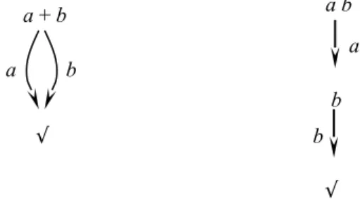
The elementary notion of the Basic Process Algebra is the notion of an atomic action that represents a behaviour, which description does not include operators of Basic Process Algebra, i.e. indivisible (has no structure) for the language of Basic Process Algebra. That is a single step such as reading or sending a data, renaming, removing etc. Let A is a set of the atomic actions. Atomic action is supposed to be internally non-contradictory, i.e. each atomic action v also can be considered as an algorithm, which can execute it, and always terminates successfully. It could be expressed either by process graph:
or by the predicate v √. Here the atomic action in the node (or on the left side of predicate) we can consider as a program code, and the atomic action to the left from the arc (above the arrow) as an execution or run of that code. We will not involve the processes that do not terminate.
The notion of process term is the next inductive level of the formalism of Basic Process Algebra. v
√ v
Definition 2.1 Process term
1) An atomic action is a process term.
2) Alternative composition x + y of process terms, that represents the process, which executes either
process term xor process term y, is also a process term.
3) Sequential composition x • y of the process terms, that represents the process, which first executes the process term x, and than the process term y, is also a process term.
Each finite process can be represented by such process terms that are called basic process terms. The set of the basic process terms defines Basic Process Algebra.
2.2.2 Semantics
Intuition that underlies the definition of basic process terms can allow us to construct process graphs that correspond to these notions. By analogy with structural operational semantics (Fokkink, 2000) transition rules represented in Table 2 .1 can be obtained. Here the variables x, y, x’, y’ are from the set of basic process terms, while v – from the set of atomic actions.
Table 2.1 Transition rules of Basic Process Algebra
v √
x √
x + y √
x x’
x + y x’
y √
x + y √
y y’
x + y y’
x √
x • y y
x x’
x • y x’• y
a b
b a
√
b
Figure 2.2 Process graphs of alternative and sequential compositions
a + b a
√
The first transition rule expresses that each atomic action can terminate successfully by executing itself. The next four transition rules are for alternative composition and show that it executes either x or y. The last two transition rules correspond to sequential composition and show that in that case first the process x has to be terminated successfully; only after that the process y can be started. Note that the execution of y is probably to involve another transition rule; the rules for sequential composition do not execute second term. It is a good support of the idea that the right distributive law does not satisfy to Basic Process Algebra.
2.2.3 Bisimulation Equivalence
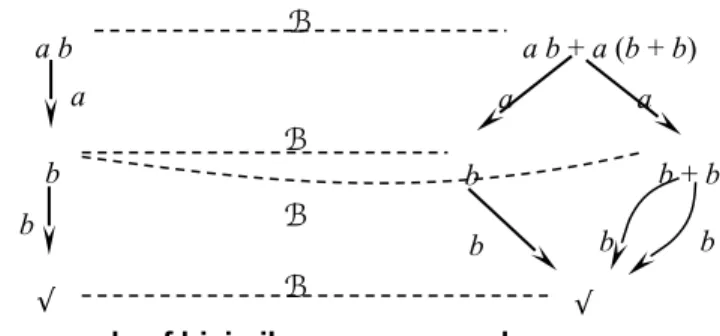
Basic Process Algebra does not conclude that two processes are equal if they can execute exactly the same strings of actions (trace equivalence). As a reason we can look at the example of the graphs in Figure 2.1 that depict the law of right distribution. If we look at an alternative composition such as an example of choice function, then it becomes substantial where to make a decision: before the reading of data or after.
In spite of trace equivalence, bisimulation equivalence also pays attention to the branching structure of the processes.
Definition 2.2 Bisimulation
A bisimulation relation ℬ is a binary relation on the processes such that:
1. if xℬ y and x x' , then y y' with x ' ℬ y'
2. if xℬ y and y y' , then x x' with x ' ℬ y'
read (data) read (data) read (data)
forward (data) delete (data) forward (data) delete (data)
Figure 2.3 Graph’s analogy of right distributive law. The two graphs are not bisimilar. √
√
Figure 2.4 An example of bisimilar process graphs.
a b
b a
√
b
a b + a (b + b)
b a
√
b
b + b
b b
a
ℬ
ℬ
ℬ
3. if xℬ y and y √, then x √
4. if xℬ y and y √ , then x √
2.2.4 Axioms
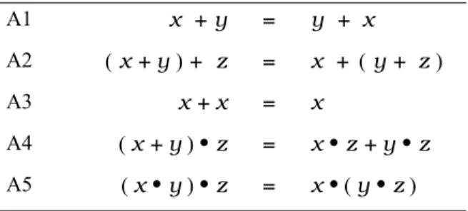
Basic Process Algebra has a modulo bisimulation equivalence sound and complete axiomatisation, written down in Table 2 .2 (Fokkink, 2000).
Table 2.2 Axioms for Basic Process Algebra
A1 x + y = y + x
A2 (x + y ) + z = x + (y + z )
A3 x + x = x
A4 ( x + y) • z = x • z + y • z A5 ( x • y) • z = x • ( y • z )
2.3 Operators of Process Algebra for parallel processes
Process algebra involves parallelism that is both non-communicative and communicative. There are several operators to express the idea of parallelism that can be treated quite widely. At first sight it is possible to find a kind of parallelism even in the alternative composition that is one of the operators of Basic Process Algebra and represents an action, which can choose an execution of one of the two process terms. However alternative composition can be considered as parallel only in stasis that is before choice when we have two “parallel” branches – two potentials. But during execution we will have a trace only via one branch, and all “parallelism” disappears.
2.3.1 Free merge or parallel composition
A new idea (in comparison with Basic Process Algebra) was used in the free merge operator or parallel composition introduced by Milner (1980). Free merge allows us to execute two process terms in parallel. Table 2.3 Transition rules of Free Merge
x √
x || y y
x x’
x || y x’ || y
y √
x || y x
y y’
x || y x|| y’
composition, an execution of the right process can be started before the termination of the left one. Semantics of free merge can be expressed by the transition rules represented in Table 2.3. Whereas x √ represents a successful termination of the process term x after the execution of an atomic action v,
x x’ means a partial successful termination of the process term x with the remaining part x’ after the
execution of an atomic action v. The variables x, x’, y, and y’ range over the collection of the process terms, while v ranges over the set A of the atomic actions.
Free merge can be treated as a superposition of two operators of left merge, which we will describe at the next subsection. Unfortunately, Process Algebra with free merge has not finite sound and complete axiomatisation. This fact was proved by Moller (1990).
2.3.2 Left merge
Left merge can be considered only as a decomposition of free merge. It has not an independent semantics. Indeed, if we would take an idea of left merge independently from free merge, then we will provide semantics already expressed by operator of sequential composition. Transition rules for left merge are in the table 2.4.
Table 2.4 Transition rules of Left Merge x √
x ⌊⌊ y y
x x’
x ⌊⌊ y x’ || y
From tables 2.1, 2.3 and 2.4 axioms for the free and left merges follow Table 2.5 Axioms for the Free and Left Merges
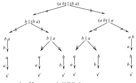
FM1 x || y = x ⌊⌊ y + y ⌊⌊ x Figure 2.5 Process graphs of free merge (a b) || (b a)
(a b) || (b a)
a b
b || (b a) (a b) || a
b b
b a b || a
a a
b || a a b
√
b a
a b
b a
a b
a
√
b
√
b
√
a b
√
a a
a
√
LM1 v ⌊⌊ y = v • y LM2 ( v • x )⌊⌊ y = v • ( x || y ) LM3 ( x + y )⌊⌊ z = x ⌊⌊ z + y ⌊⌊ z
From the axioms of table 2.5 is clear to see that each term of Process Algebra for parallel processes can be rewritten by equivalent Basic Process Algebra’s term.
2.4 Operators of Process Algebra for communicating processes
Process Algebra for communicating processes contain extension of free merge for parallel processes. The new operator we will call merge, or parallel composition. Besides the features of free merge it can execute two process terms simultaneously. For that purpose communication function will be introduced in subsection 2.4.1 , which governs the executions of communication merge. Process algebra for communicating processes is sound and complete (Moller, 1990).
2.4.1 Communication function
The notion that can explain the mechanism of interaction in Process Algebra and outline the issue of communication merge is communication function. This function is a partial mapping : AAA, where A is the set of the atomic actions. It is easier to understand the meaning of the function by the following send/ read example.
Send/read communication As follows from the definition the construction of the communication function is possible if there are three atomic actions in the atomic action set, such that we can map two of them on to the third one. In order to fulfil that condition in case of the send/read communication it is enough to have a send action s(d),a read action r(d), and a communication action c(d) for the data d that corresponds to the send and read actions and expresses the process of information exchange. Communication function is
(s(d), r(d)) = c(d). I suppose the function was introduced because we prefer to operate with one process during one step of time and to stay at one state after the execution, that is a standard intention, and the communication function provides the possibility to do it. Indeed, it is impossible to follow several branches of a graph (by which the parallel processes can be represented) simultaneously and to stay at several states.
2.4.2 Communication merge
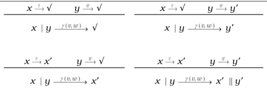
Table 2.6 Transition rules of Communication Merge x √ y √
x | y √
x √ y y’
x | y y’
x x’ y √ x | y x’
x x’ y y’
x | y x’ || y’
Communication merge is an extension of communication function. It is clear from the following axioms a | b= (a, b) , if (a, b) defined, CF1
a | b = otherwise. CF2
Here is a deadlock; that means that the processes have stopped its execution and can not proceed. The other axioms for communication merge are represented below.
Table 2.7 Axioms for Communication Merge
CM1 v | w = ( v, w )
CM2 v | ( w • y ) = ( v, w ) • y CM3 ( v • x ) | w = ( v, w ) • x CM4 ( v • x ) | ( w • y ) = ( v, w ) • ( x || y) CM5 ( x + y ) | z = x | z + y | z CM6 x | ( y + z ) = x | y + x | z
2.4.3 Merge
As we mentioned, merge is an extension of free merge and is expressed through represented parallel operators by the following axiom.
M1 x || y = x⌊⌊ y + y⌊⌊ x + x | y
2.5 Conclusion
As is apparent from this chapter, Process Algebra has an interesting realisation of the concept of parallelism. Since Basic Process Algebra has analogues for two basic operators of Game Logic, it could rise optimistic prospects in the extension of Game Logic by parallel operators of Process Algebra. However, Process Algebra does not contain a notion of dual game, and its encapsulation would look unnatural. Besides, the possibility of expression of true-false values in Process Algebra looks doubtful. Moreover, it seems that Process Algebra does not support an ideology of two-player game. So, the encapsulation of parallel operators of Process Algebra in the theory of Game Logic is not obvious. However, we will use Process Algebra to discuss some properties which are not represented directly in semantics of tensor and par operators of Linear Logic described in the next chapter. It is analogues of tensor and par operators we will use to extend Game Logic on parallel operators.
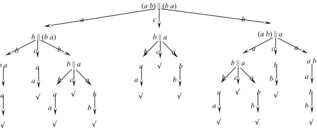
Figure 2.6 Process graphs of merge (a b) || (b a). Here c is a communication of two atomic actions from {a, b}.
(a b) || (b a)
a b
b || (b a) (a b) || a
b b
b a b || a
a a
b || a a b
√
b a
a b
b a
a b
a √ b √ b √ a b √ a a a √ b b c
b || a
b a
a b
3 Parallel games in Linear Logic
As explained, Linear Logic can have a game theoretical interpretation. The semantics given by Blass (1992) relates to Affine Logic. Affine Logic can be obtained from Linear Logic by adding the structural rule of weakening. His semantics was criticised by Abramsky and Jagadeesan (1994), who introduced another game semantics sound and full complete with respect to multiplicative fragment of Linear Logic. Since we consider the games merged by the multiplicative operators as parallel, the conceptual similarity between semantics for additive fragment of Linear Logic and Game Logic allows us to predict the possibility of extension of Game Logic by means of analogues of multiplicative operators of Linear Logic.
3.1 Introduction
In this chapter, the basic features of the games involved by Blass and Abramsky, Jagadeesan are listed in section 3.2 . Since we are going to use the properties of multiplicative operators to enrich the language of Game Logic, in section 3.3 we fulfil in special manner an interpretation of Linear Logic connectives by operations on games. For this purpose we took the basic ideas from Blass and Abramsky, Jagadeesan semantics.
3.2 The game semantics for Linear Logic
Abramsky and Jagadeesan oppose their semantics to that of Blass because they argue with him about the completeness theorem. In any case, we have not need to follow this line because we can not convert a semantics of Linear Logic to the semantics of Game Logic without changes. It is enough to look at the definition of -strategy (Chapter 4), which is used in Game Logic instead of notion of winning strategy of
Linear Logic. Thus, we can try to make a quintessence of the two semantics and postpone the restrictions on the moment of definition of soundness and completeness inside a model of Game Logic.
3.2.1 The origin of Blass’s game semantics for Linear Logic
The Blass’s (1992) game semantics for Linear Logic arose over reconsideration of Lorenzen’s (1959) game semantics for Propositional and First Order (Classical) Logic. Lorenzen’s game semantics includes procedural conventions, which bring asymmetry between players. There is a reason to avoid such structural difference between axiomatics and semantics: logical connectives have a symmetrical status in the axioms and rules of inference, whereas Lorenzen's game semantics has the asymmetrical conventions. In Table 3 .5 there is a brief description of updates, which Blass (1992) offered to avoid the asymmetry of Lorenzen’s procedural conventions. One of the asymmetry eliminates by introduction of undetermined games.
Definition 3.1 Undetermined games
Table 3.5 Blass's elimination of the players’ asymmetry
Lorenzen’s procedural
convention Blass’s transformations
Proponent may only assert an atomic formula after Opponent has asserted it
Every atomic game has to be
undetermined
Permission or restriction on re-attack (re-defence)
Add extra sort of conjunction (disjunction)
The other asymmetry disappears by using the expressive power of the language of Linear Logic. In Linear Logic there are two sorts of conjunction and disjunction: additive and multiplicative. In Blass’s game semantics additive conjunction (disjunction) does not allow to re-attack (re-defence), whereas multiplicatives do allow this.
3.2.2 Basic notions of Game Semantics
There are two basic notions in game semantics: game and winning strategy. We give key moments of their definitions, which we constructed according to the general view of Blass and Abramsky, Jagadeesan. Below we summarise the main properties of the involved games.
1. 2-players: Proponent (P), and Opponent (O) 2. Zero-sum (strictly competitive - either P or O wins) 3. Undetermined atomic games; we can get it by:
infinite branches (in Blass (1992) semantics)
imperfect information (in Abramsky and Jagadeesan (1994) semantics; they operate with history-independent strategies (a current move depends only from the previous one))
Definition 3.2 Game
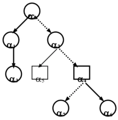
A game A depicted by game tree drawn in Figure 3.1 is a quadruple (MA , A , PA , WA ), where 1) MA = {0, 1, …, 7 } - the set of possible moves in game A, where 3, 5, 6, 7 may or may not
be the last moves of the game in Figure 3.1. A Greek letter at state on the tree is a name of the last executed move (0 is a name for an empty move).
2) A : MA {P,O} - labelling function distributing the set of possible moves in game A between the
players. A square or circle at a state of the tree shows who has to move at the next turn.
moves (stressed by bold arrows). The uniqueness of the combination of moves means that we can not reach a position by the different branches of a tree. That is why the graph has no loops. 4) WA - the winning branches, by which Proponent can achieve a victory (drawn in dash)
Definition 3.3 Strategies
Strategy of a player in game A is a function into MA , from the set of all positions where the player has to move. The strategy is a winning one if all branches of are in WA .
Eventually, a player can have winning branches and no winning strategy. However, if the player has a winning strategy then she has winning branches.
3.2.3 Winning strategies in Blass's semantics
Important feature of Blass semantics is an absence of winning strategies for the atomic games. It gives the following results (that you can find out from section 3.3 ).
1) Games without multiplicative connectives and repetitions do not contain winning strategies for either player. And hence we can not distinguish such games if we would include an outcome of game in game definition
2) If we add a multiplicative part to games then we can obtain winning strategies 3) The known winning strategies are only different sorts of copy strategy
4) When we will refer during following discussion that, for instance, in game A B one of the players has a winning strategy in game A, it will mean that A is not an atomic game and contain multiplicative connectives together with a copy strategy for that player
5) Without copy strategy (even if we suppose winning strategies in atomic formula) multiplicative operators on games would not distinguished from additive one.
0
1 2
3
Figure 3.1. A game tree with the set of possible moves {0, 1, …, 7 }. The set of moves of
Proponent is pointed out by squares, of Opponent - by circles. The set of valid positions (admissible moves) stressed by bold, whereas winning branch for Proponent by dash.
5 4
3.3 Game interpretation of the operators of Linear Logic
Since the goal of the introduction of the game semantics is its adaptation to the Game Logic, we will make the following definitions on the special manner that could be considered as transitional.
Definition 3.4 Negation
A = ( MA , A , PA , \ WA )
Here we change only scheduling and the goals by switching between two-player.
Winning strategies
A winning strategy (if it exists) of one of the players in game A becomes the winning strategy of another player in dual game A.
Definition 3.5 Additive conjunction
A B = ( MA B , A B , P A B , W A B )
Where:
MA B = MA + MB + {0,1} (if 0 then choose component A, if 1 then choose component B) A B = A + B + (0, O) + (1, O) , i.e. Opponent choose which game to play
P A Bis the union of the sets P Aand P Bthrough prefix position such that: 1) The restriction to moves in MA (respectively MB ) is in PA (respectively PB ) 2) Opponent has to choose in the prefix position which game to play
W A B is the union of the sets W A and W B through prefix position Winning strategies
Proponent has a winning strategy in compound game if she has winning strategies in both components. Opponent has a winning strategy if he has it in one of the components.
Definition 3.6 Additive disjunction
A B = ( A B )
It gives the switching of roles between Opponent and Proponent
Winning strategies
Proponent has a winning strategy in compound game if she has winning strategies in one of the components. Opponent has a winning strategy if he has it in both components.
The general significant difference of semantics' description for multiplicative connectives compared to the additive one is that we will use multi-states to express a compound game.
Definition 3.7 Multiplicative conjunction (Tensor)
0
1 2
0
1 2
3
(0, 0)
(1, 0) (2, 0) (0, 1) (0, 2)
(3, 0) (1, 1) (1, 2) (2, 1) (2, 2)
(3, 1) (3, 2)
(3, 1) (3, 2)
(1, 1) (2, 1)
(3, 1)
(1, 2) (2, 2)
(3, 2)
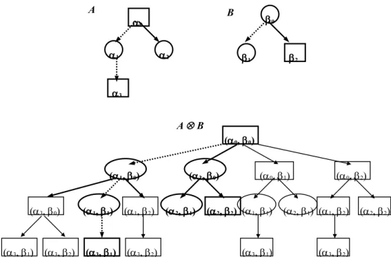
Figure 3.2. The set of all possible moves in compound game with a multiplicative connective is the following partial Cartesian product of the two component games
0
1 2
0
1 2
3
(0, 0)
(1, 0) (2, 0) (0, 1) (0, 2)
(3, 0) (1, 1) (1, 2) (2, 1) (2, 2)
(3, 1) (3, 2)
(3, 1) (3, 2)
(1, 1) (2, 1)
(3, 1)
(1, 2) (2, 2)
(3, 2)
A B
A B
MA B is the partial Cartesian product of two possible moves' sets MA and MB, as is shown in
Figure 3.2. It is constructed as follows. Take the initial states of the component games (proto-states) and make from them an initial complex state. Construct the complex states of the next level by fixing consecutively each of the proto-state of initial complex state and taking successors of another one from the component game. By applying that procedure to each complex state we can construct a multiplicative tree of the set of possible moves.
A B labelling function: it is Opponent’s turn to move if and only if it is her turn to move in both
games, otherwise it is Proponent’s turn to move
PA Bis the set of valid positions (admissible moves) that constructed as follows:
1) If it is Opponent’s turn to move she can move in any possible direction (during her turn she is allowed to move in both components, and hence she can always switch the game)
2) If it is Proponent’s turn to move he can move only in the component where it is his turn to move (note that if he has turn to move in both components, he can switch the games)
WA B is the set of all winning for Proponent branches that equal to intersection of the winning
branches of the component games (i.e. Proponent has to win in both components of the resulting multiplicative branch).
Winning strategies
Proponent has a winning strategy in compound game if he has winning strategies in both components. Opponent has a winning strategy if she has it in one of the components. Besides, Opponent can have a winning strategy in compound game even if nobody has winning strategies in component games and, at the same time, she can apply one of the copy strategies. For instance, a copy strategy can be applied by Opponent (she can switch between two games and hence to copy moves from one to another) if we have a compound game A A . Another opportunity of applying a winning strategy for Opponent is a game AA over nonprincipal ultrafilter on the set of natural numbers (see, for instance, Blass 1992).
Definition 3.8 Multiplicative disjunction (Par)
Par – is the game combination AB = ( A B ), where (see Figure 3.3):
MA B = MA B
A B labelling function: Proponent has to move if and only if he has to move in both games,
otherwise Opponent has to move
PA Bis the set of valid positions (admissible moves) constructed as follows:
1) If it is Proponent’s turn to move he can move in any possible direction (during his turn he is allowed to move in both components, and hence he can always switch the game)
WA B is the set of all winning for Proponent branches that equal to union of the winning branches
of the component games (i.e. for Proponent enough to win in one of the components of the resulting multiplicative branch).
Winning strategies
Proponent and Opponent switch the roles in comparison with the tensor games.
3.4 Games with several multiplicative operators
The multiplicative operators yield complex states that were considered in previous section. It can give rise to the following questions:
how to determine who has to move in such games,
in which components the player can switch.
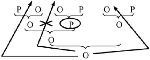
The first question has quite an evident answer: we have to count from the lowest level of sub-games whose turn it is to move according to atomic game schedule and multiplicative connectives. An example of such a counting is depicted in Figure 3.4.
The next question is easier to find out now we have an answer to the first one. A player can make a switch to those atomic games where both she/he has a move and in each subformula of main formula that include this game she/he also has to move. See Figure 3.5.
O P P O O O
O
Figure 3.4 Labelling function for games with several multiplicative operators
P O O P O P O P O
O . O
Figure 3.5 Admissible atomic plays for switcher Game:
A, A, B , B :
A A , B B :
4 An extension of Game Logic with Parallel Operators
Linear Logic has two-player game semantics, and contains multiplicative operators: tensor and par. Game Logic arose from Propositional Dynamic Logic and was introduced by Parikh (1985) as a language to explore games.
The language of Game Logic has two constituents, formulas (propositions) and games. A set of atomic games 0 and a set of atomic formulas 0 are at the basis over which we can define games and
formulas (Pauly, 1999):
g | ? | ; | | * | d
| p | | |
where p0 and g 0. Also the following equations are valid
Т ,
[] ,
(),
.
In the chapter we introduce semantics, syntax and axiomatics of parallel operators for Game Logic, basing on definitions for multiplicative operators of Linear Logic.
4.1 Preliminaries
This section contains general mathematical definitions, which will be used in this chapter.
Multiset is a set-like object in which order is ignored, but multiplicity is explicitly significant. Therefore, multisets {1, 2, 3} and {3, 1, 2} are equivalent, but {1, 2, 3} and {1, 1, 2, 3} differ. Given a set
S, the power set of S is the set of all subsets of S. The order of a power set of a set of order n is 2n. The
power set of S can be denoted as 2S or P(S).
List is a data structure consisting of an ordered set of elements, each of which may be a number, another list, etc. A list is usually denoted (a1, a2, ..., an) or a1, a2, ..., an, and may also be interpreted as a vector. Multiplicity matters in a list, so (1, 1, 2) and (1, 2) are not equivalent. Proper List is a prefix of list, which is not the entire list. For example, consider a list 1, 2, 3, 4. Then 1, 2, 3 and 1 are proper subsets, while 1, 2, 3, 4and 1, 2, 5 are not. If p and q are the lists, then q < p will denote that q is a proper list of
p. The notation q ≤ p is conventionally used to denote that q = p, or q < p. A list x of the set of lists S is a maximal list of the set of lists if and only if it is not a proper list of any list from the set.
and n - 1 edges is a tree. Maximal Sub-Tree for given node of tree is a tree that contains all sub-branches, starting from the given node of the initial tree.
4.2 Game model and game structures
In this section we define a game structure. It is a formal general definition of game. The definition is adapted to application with the parallel operators. For this purpose we involved specified mask function. Besides, we discuss the differences between winning strategy and -strategy, which is an extension of
winning strategy for a game model of Game Logic. At the end of the section we define the game model for Game Logic with Parallel Operators.
4.2.1 Game structure
We consider the games between Proponent (P) and Opponent (O), and define a game tree as a following
game structure.
Definition 4.1 Game structure
A game structure G is defined by the tuple (S, M, , , R,P, O), where 1) S = {s0, s1, …, sn } is a finite set of states
2) M = {m0, m1, …, mk}is a finite set of all possible atomic moves
3) R = {q0, q1, …, qh}is a set of admissiblesequences of moves (histories, or branches) ;
a sequence of moves is a list
If qR and p ≤ qthenpR
4) : R Sis a trace function defining a state that we can achieve by fixed history
5) : S {P, O, E} is a scheduling function, which determines for each state who has to move at the next turn; for all final states f, which have no successors: f = E
6) P: S {⊤, ⊥} is a specified mask function for Proponent 7) O: S {⊤, ⊥} is a specified mask function for Opponent
A part of a sequence of moves we will call a segment if only one player has moves inside this part.
Example of a game tree.
In Figure 4.1 we depict a general example of game tree. Game structure in this case has the following content.
1) S = {s0, s1, s2, s3, s4}
2) M = {m0, m1, m2}
3) R = {, m0, m1, m0, m2, m1, m0, m1, m1}
4) () = s0; (m0) = s2; (m1) = s1; (m0, m2) = s3; (m1, m0) = s3;
(m1, m1) = s4
5) (s0 ) = P; (s1 ) = O; (s2 ) = O; (s3 ) = E; (s4 ) = E
6) P(s
3) = ⊤; P(s0) = ⊥; P(s1) = ⊥; P(s2) = ⊥; P(s4) = ⊥
7) O(s
4) = ⊤; O(s0) = ⊥; O(s1) = ⊥; O(s2) = ⊥; O(s3) = ⊥
Game structure can be applied to the different types of game. Later on we will present axioms for given semantics, but the axioms are not valid for all types of game. Below we express necessary types through the given game structure.
Besides, during further discussion, we will call a taken sequence of moves x, such that p: pxR
psx=E, a play of game from given state s.
Definition 4.2 -zero-sum game
A game is a -zero-sum from given state s =
p if and only if
qR pqq = E rR prr qP
r = ⊤O r = ⊤
Remark. Why -zero-sum
We call such type of games -zero-sum because it seems to use an ideology of zero sum game
taken from the games which use a terminology of winning strategies and applied to the games with language of -strategy (see Definition 4.7 below). The idea is that two-player can not loose or win
m0
s0
s1
s3
s2
m1
m2
Figure 4.1 A game tree. The set of states is represented by circles (with Opponent turn to move), squares (with Proponent turn to move), and points (nobody has to move). Arrows represent the set of moves. Bold arrows show Proponent’s -strategy.
m0
s4
s3
m1
simultaneously, but may have a draw. In our case, we consider reaching a state where is valid for either player (or in other words, that function is determined for both players) as a draw that is quite naturals. Therefore we follow the idea of zero-sum games.
Definition 4.3 Determined and undetermined games
A game is determined from given state s if and only if it is possible, starting from that state, to present a -strategy (see Definition 4.7 below) for one player or a -strategy for the other
(). Otherwise the game is undetermined from given state s.
4.2.2 Winning branch and winning strategy
The notion of winning strategy plays key role in the semantics of game theory. For given game structure
it is possible to determine a set of winning states or a set of winning sequences of moves for each player: WP, WO. Player can achieve a winning position (state) of a game under the influence of different reasons.
If it happens because her/his competitor made a mistake during the game, then we can say that the winner has a winning branch, which he followed at the game. If the player can achieve a winning position irrespective of mistakes of the competitor then we can say that the player has a winning strategy.
Game structure, defined in subsection 4.2 , allows us to play games not only from the initial state; for instance, in chess we have an opportunity to decide endgame problems. It can be useful, because even if we could not find a winning strategy for either player in full chess game, we can find a winning strategy in most of chess endgames. Therefore, below we give precise definitions of the ‘strategic’ notions, which can be considered from the given state of a game.
Definition 4.4 Winning branch for the given state s
Player N{O, P} has a winning branch in the game starting from state s if and only if there is a sequences of moves p in game such that s = (p) and there is x such that px WN.
Definition 4.5 Winning strategy for the given state s
Player N{O, P} has a winning strategy in game starting from state s if and only if
p R ((p)=sT = {x: pxR y x (((py)) = N m1, m2 M z1, z2
(ym1z1 R ym2z2 R) x = (ym1z1 ym2z2))} x (xT ((x)) = E)
pxWN)
The subtree T is a winning strategy for the given state.
Consider apart the formula given in Definition 4.6. We begin a game from state s =(p) that has to be reached by admissible sequence of move p. We are looking for the tree T that starts from state s and copies all admissible sequences of moves of subtree pxR except in those which are the alternatives for
the player N moves ((py)) = N m1, m2 M z1, z2 (ym1z1Rym2z2R) x = (ym1z1
ym2z2). Besides, all maximal sequences of moves of the tree has to be in winning set of player N: x
(xT((x)) = E) pxWN).
4.2.3
-strategy
For application in game models we have to extend the notion of winning strategy to the notion of
-strategy. But first we determine the notion of X--strategy.
Definition 4.6 X- strategy for the given state s
Player N{O, P} has an X-strategy in game starting from the state s if and only if it is possible to construct a winning strategy for the player from the state s, which all outcome states would belong to X, where X is a set of states.
Definition 4.7 I- strategy for the given state s
Player N{O, P} has an -strategy in game starting from the state s for model I if and only if
she/he has an X-strategy, and for all states sX and all their successor states (if their exists):
I,s ⊨ .
Notion of -strategy plays key role in definition of game model and hence in validity of axioms. Therefore,
consider how -strategy can occur at the games.
Each player can have in a game -strategy, or -strategy (where ), or both of them, or
nothing.
Definition 4.8 Strategy couple
Determine a strategy couple as (X, Y) , where X is a set of strategies which has Proponent in game , starting from the state s0 (namely -strategy, or -strategy (where ), or both of them,
or nothing), and Y – for Opponent.
Definition 4.9 Shadow of strategy couple
We will call a Boolean quadruple shadow of strategy couple if it is the following projection of the strategy couple:
first element of tuple is true if Proponent has a -strategy; otherwise it false,
second element is true if Proponent has a -strategy; otherwise it false,
third element is true if Opponent has a -strategy; otherwise it false,
fourth element is true if Opponent has a -strategy; otherwise it false.
First, consider the cases when a game starts from the last node. We assume that in each state of the game either function is valid or its negation, but not both of them. We supposed that ; then we have to check only the combinations of states where the functions are valid and of the players moves as it is depicted in Figure 4.2. In game Proponent has -strategy {m
0}, and -strategy {m1}, whereas
Opponent has none (the shadow of strategy couple for this game is (⊤, ⊤, ⊥, ⊥)). In game the picture is opposite (the shadow of strategy couple for this game is (⊥, ⊥, ⊤, ⊤)). Games and (as and ) are equal in this sense. In Proponent has -strategy {m
0, m1} and Opponent has the same (the shadow of
strategy couple for this game is (⊤, ⊥, ⊤, ⊥)). In Proponent has -strategy {m
0, m1} and Opponent
has the same (the shadow of strategy couple for this game is (⊥, ⊤, ⊥, ⊤)). m0
s0
s1
s2
m1
Figure 4.2 Occurrences of -strategy and -strategy (where ) in a game when the game starts from the last node.
({{m0},{m1}}P,
{}O)
m0 s0 s1 s2 m1
({}P,
{{m0}, {m1}}O)
m0 s0 s1 s2 m1
({{m0, m1}}P, {{m0, m1}}O)
m0 s0 s1 s2 m1 m0 s0 s1 s2 m1
({{m0, m1}}P, {{m0, m1}}O)
m0
s0
s1
s2
m1
Figure 4.3 Occurrences of -strategy and -strategy (where ) in a game when the ({{m0X, m1X}
{m0X, m1X}}P, {}O)
m0 s0 s1 s2 m1
({{m0X, m1X}
{m0X, m1X}}P, {}O)
m0 s0 s1 s2 m1
({}P, {{m0Y, m1Y}
{m0Y, m1Y}}O)
1 2 3
m0
s0
s1
s2
m1
({}P, {{m0Y, m1Y}
{m0Y, m1Y}}O)
4 m0 s0 s1 s2 m1 5
({{m0X}{m0X}}P,
{}O)
m0 s0 s1 s2 m1 6
({}P,
{{m1Y}{m1Y}}O)
m0
s0
s1
s2
m1
({{m0X, m1X}}P,
{{m0Y, m1Y}}O)
7 m0 s0 s1 s2 m1
({{m0X, m1X}}P,
{{m0Y, m1Y}}O)
8 m0 s0 s1 s2 m1
({{m0X}, {m1X}}P,
{ }O)
9 m0 s0 s1 s2 m1
({}P, {{m0Y},
{m1Y} }O)
10 m0 s0 s1 s2 m1
({{m0X, m1X},
{m0X} }P, {}O)
11 m0 s0 s1 s2 m1
({m1X}}P,
{{m1Y} }O)
12 m0 s0 s1 s2 m1
({}P, {{m0Y, m1Y},
{m0Y}}O)
13 m0 s0 s1 s2 m1
({m1X}}P,
{{m1Y} }O)
14
({{m0X},
{m0X, m1X}}P, {}O)
Next, examine the general case. Consider the nodes, which lead to the games with shadows of strategy couples as we had in Figure 4.2. Let us check whether any combination of such games gives a new shadow of strategy couple. In Figure 4.3 we draw up a sufficient amount of graphs to see that any combination of games does not give a new shadow of strategy couple. For instance in game
1 Proponent
has a -strategy {m
0X, m1X} and -strategy {m0X, m1X} whereas Opponent has none;
hence, the shadow of strategy couple for this game is (⊤, ⊤, ⊥, ⊥) which is equal to the shadow of strategy couple for game . It is easy to see that we can not obtain a new shadow of strategy couple without special assumptions. Now we can make the following claim.
Claim 4.1 Shadow of strategy couple for determined games
The shadows of strategy couple for finite determined games have the following values: 1) (⊤, ⊤, ⊥, ⊥)
2) (⊥, ⊥, ⊤, ⊤) 3) (⊤, ⊥, ⊤, ⊥) 4) (⊥, ⊤, ⊥, ⊤)
Obviously we can not have a shadow like (⊤, ⊤, ⊥, ⊤) or (⊤, ⊤, ⊤, ⊤) anytime, because it is impossible that Opponent would have a -strategy whereas Proponent has a -strategy. Indeed, the fact that one
player has a strategy to achieve a goal entails that the other player can not achieve an opposite goal. However, the four represented cases are not enough to express the features of parallel operators (section 4.3.2 ) that we will discuss in subsection Claim 4.2. The reason is a copy strategy that players do not need if they have any other strategy in the playing game. Thus, to have a reason to apply a copy strategy we have to find a way of appearance of shadow in form (⊥, ⊥, ⊥, ⊥).
Such a shadow can appear in infinite games, like it is shown in Figure 4.4 game , and in games with imperfect information shown in game . In such games we can also obtain a shadow for which only one element is true. In case of , if we assume that s2 is final state and is valid in the state then we obtain
the shadow of strategy couple (⊤, ⊥, ⊥, ⊥). In case of , if we predetermine that in state s4 is valid then
we obtain the shadow of strategy couple (⊥, ⊥, ⊤, ⊥).
Claim 4.2 Shadow of strategy couple for undetermined games
The shadows of strategy couple for undetermined games can be equal to one of those of determined games or one of the following:
1) (⊤, ⊤, ⊥, ⊥) 2) (⊥, ⊥, ⊤, ⊤) 3) (⊤, ⊥, ⊤, ⊥) 4) (⊥, ⊤, ⊥, ⊤)
4.2.4 The role of copy strategy in model distinction of operators
In this subsection all discussion will concern -zero-sum games for parallel operator, which are played
from the given state. It does not mean that the games, which constitute a parallel game, have to be
-zero-sum. That would be confirmed by the Figure 4.6 if you will predetermine function P or O for state s
2 of
game .
First of all consider the influence of the assumption that the game structure is determined on the semantics of parallel operators. If a game is determined then for a given game we can say in advance whether a player has a -strategy for this game or not. This means that we do not need to appeal to the
peculiarity of parallel operators that lies in switching between the games to find a -strategy. If a player
knows in which game she/he has a -strategy, she/he can choose the game immediately. Furthermore, it
m0
s0
s2
m1
Figure 4.4 The cases when the shadow of strategy couple is equal to (⊥, ⊥, ⊥, ⊥). ({}P, {}O)
m0 s0 m1 m0 s1 s6 s5 m1 m0 s3 m1 m0 s1 s5 m1 m0 s4 s8 s7 m1
m0
s11
m1
m0
s12 s15 m1 m0 s10 m1 m0 s13 m1 s14 m0 s0 s2 m1 m0 s2 s4 s3 m1
({}P, {}O)
s6
parallel operators , respectively. The opportunity to leave one of the two component games of a parallel operator without playing gives rise to the equivalence.
If we suppose that the involved games are undetermined then the search of -strategy for choice
operators reminds us of a Russian Roulette: when pulling the trigger you do not know what you will get either a bullet or a Muscovite maiden. On the contrary, switching function of parallel operators gives a chance to impress the Muscovite maiden without being shot through brains. The chance is based on the external, towards the atomic game structure, procedures of constructing -strategy. We will call such
-strategies structural. The well-known copy strategy is one of them. Obviously, if Opponent will play
when the components of tensor are undetermined games, and if she/he copies moves of one game to another then it gives a -strategy, and it is a copy strategy.
Consequently, we found that the structural -strategies contain peculiarity of parallel operator
towards the operators of choice. However, the appearance of structural -strategies for semantics of the
parallel games causes delicacy in definition of the axiomatics. Semantics of game model is supported by the notion of an existence of -strategy for the game. Structural -strategies are components of
-strategy; hence they provide an indirect influence on the game model. On the other hand, the structural
-strategies are not completely determined. Nobody can protect against inventions of new structural
-strategies inside the determined structures of parallel games. In this way, even if we will find a sound and complete axiomatics for the given structural -strategies, the invention of a new one can not guarantee that
we will save the completeness of axiomatics.
4.2.5 Game model
In the basis we put the game semantics introduced by Pauly (1999) for Game Logic without parallelism. Given a game modelI = (S,{G(a, s) | a 0 and sS}, V ) , where S is a set of states, G(a, s) are game structures (determined dynamic games) on S, V 0 P (S) is the valuation function, define truth in a game model:
I , s ⊨ p iff p 0 and s V ( p ) I , s ⊨ iff I , s ⊭
I , s ⊨ iff I , s ⊨ or I , s ⊨
I , s ⊨ [] iff Opponent has a - strategy in game G(, s) I , s ⊨ iff Proponent has a - strategy in game G(, s)
where {sS | I , s ⊨ }.
Game structure defined above can be included in the definition of game model as follows. In our notation G(, s) is a game that is played from the given state s, and which is determined by correspondent game structure. States of the model are equal to the states of game . We can establish the strict connection between valuation function V 0 P (S) and specified mask functions for Proponent P: S {⊤, ⊥}
suppose that player N has a winning strategy in game G(, s). If we will choose a valuation function V P (S) such that it is determined for at least all states that are outcome states of the winning strategy then the player N will have a -strategy in the game. Consequently, the valuation function can be connected
with outcome states of the winning strategy. The states, in turn, depend on the specified mask functions.
4.3 Game operators for game structure
4.3.1 Non-parallel operators
Below we define some basic operators of Game Logic in terms of game structure determined in previous section.
Definition 4.10 Dual game
Dual game = d is a game structure, which can be obtained from the structure of game after the
switching of functions and between the players as follows:
sS: s = Ps = O
s = Os = P
s = Es = E
P
(s) O (s)
O
(s) P (s)
Remark. Effect of don the expression of winning, -strategies.
There is a fundamental game theoretic idea that if a player can succeed in a game, then her/his competitor can succeed in the dual game. Let us look at the effect of this idea on the expression of winning and -strategies, and game structure for non-parallel games.
1) If we talk in terms of a winning strategy, then in dual game objects of interests of Proponent and Opponent remain the same, namely their own win. Meanwhile the states, which correspond to these wins, are changed (the players are interchanging by the sets of their winning branches).
2) If we talk in terms of a -strategy, the object of interest of Proponent in a game becomes the
object of interest of Opponent in a dual one (and vice versa). This means they are interested in
m0 s0 m1 m0 s1 s6 s5 m1 d m0 s2 s4 s3 m1 m0 s0 m1 m0 s2 s6 s5 m1 m0 s1 s4 s3 m1
m
0
s
m1 m0
s10
m1 m0
s
m1 m0
s10
m1
WO WP WP WO
achieving a state where is valid (or not valid). Simultaneously, the states where is valid is not changed.
From this it is easy to see that in both cases we have the same result, and it is the reason why we have a slightly different description of elements relating to winning and -strategies in game
structure. In Figure 4.5 we depicted the situation of discussed changes in dual game. As you can see, -strategies may change from correspondence with winning strategy of a player to her/his
loosing strategy even inside one model.
Definition 4.11 Test game
Test game = ? is a game structure, which satisfies to the following properties. 1) S = {s0}
2) M = {}
3) R = {}
4) () = s0
5) (s0) = E
6) P
(s0) = ⊥
7) O
(s0) = ⊤ I, s0 ⊯
Definition 4.12 Union game
Union game = ⋃ is a game structure, which satisfies to the following properties. 1) S = S ⋃ S ⋃ s⋃
2) M = M ⋃ M ⋃ 0 ⋃ 1
3) R = ⋃ 0R ⋃ 1R
4) p R: (0p) = (p)
p R: (1p) = (p)
() = s⋃
5) sS: (s) = (s)
sS: (s) = (s)
(s⋃) = P
6) sS: P(s) = P(s)
sS: P(s) = P(s)
7) sS: O(s) = O(s)
Definition 4.13 Composition game
Composition game = ; is a game structure, which satisfies to the following properties. 1) S = S ⋃ S (the states of has to be renamed for each new start from )
2) M = M ⋃ M (the moves of has to be renamed for each new start from )
3) R = R ⋃ R = {p R: ((p)) = EP((p)) ⊥O((p)) ⊥}R
4) p R - R : (p) = (p)
p R R: R (p) = (p| )
R (p) = (p)
5) sS: (s) = (s)
sS: (s) = (s)
6) sS: P(s) = P(s)
sS: P(s) = P(s)
7) sS: O(s) = O(s)
sS: O(s) = O(s)
4.3.2 Parallel operators
In this section we suppose to extend the existing language of Game Logic to parallel operators. We will introduce an analogue of multiplicative operators from Linear Logic, which were described in part 3. We have called new operators parallel; one of them is tensor, the other is par.
Analogue of Tensor game
Tensor game is a type of parallel game, in which the component games can be played alternatively and the switching between the games is governed by Opponent.
Definition 4.14 Tensor game
Tensor game = is a game structure, which satisfies the following properties.
1) S = {s = (s , s): s S , s S} is a set of the multiple states; multiple state is a multiset;
If S and S contain equal states, they have to be renamed.
2) M = M ∪ M; if and have equal names for some moves, then the moves have to be renamed
(even if = ); we need it to know to what game each instantiation belongs to. 3) R = {q: q| R q| R px (px ≤ q x M )
( ( ( p)) = (( p| )) p| px| ) for {, }