An improved method for the removal of ring artifacts in high resolution CT imaging

R E S E A R C H

Open Access

An improved method for the removal of ring

artifacts in high resolution CT imaging

Sabrina Rashid

, Soo Yeol Lee

and Md Kamrul Hasan

Abstract

In high resolution computed tomography (CT) using flat panel detectors, imperfect or defected detector elements cause stripe artifacts in sinogram which results in concentric ring artifacts in the image. Such ring artifacts obscure image details in the regions of interest of the image. In this article, novel techniques are proposed for the detection, classification, and correction of ring artifacts in the sinogram domain. The proposed method is suitable for multislice CT with parallel or fan beam geometry. It can also be employed for ring artifact removal in 3D cone beam volume CT by adopting a sinogram by sinogram processing technique. The detection algorithm is based on applying data driven thresholds on the mean curve and difference curve of the sinogram. The ring artifacts are classified into three types and a separate correction algorithm is used for each class. The performance of the proposed techniques is evaluated on a number of real micro-CT images. Experimental results corroborate that the proposed algorithm can remove ring artifacts from micro-CT images more effectively as compared to other recently reported techniques in the literature.

Keywords:computed tomography, ring artifact, sinogram, flat panel detector.

1 Introduction

Flat panel detectors (FPDs) are used to obtain high reso-lution computed tomography (CT) image. But due to technical faults of these FPDs, ring artifacts are often generated in the CT image. These artifacts may be caused by damaged detector pixels, mis-calibrated detec-tor pixels, impurities in scintilladetec-tor crystal or dust on scintillator screens. All these phenomena attribute to the generation of a number of concentric superimposed rings in the reconstructed image which correspond to stripe artifacts in sinogram domain. These rings can be of different types and of different intensities. As for example, completely damaged detector pixels cause strong isolated or band rings. Similar artifacts also arise from dusty or damaged scintillator screens [1]. On the other hand, mis-calibrated detector elements lead to less strong ring artifacts in the tomographic image [2]. These artifacts are also sensitive to tube voltage. Changes in the tube voltage alter the intensity of the ring. As these artifacts severely degrades the image

quality by obscuring significant image details, it is neces-sary to remove them, otherwise, post processing, such as noise reduction or segmentation of image information, becomes quite difficult.

There are a number of different methods to reduce these ring artifacts, e.g., hardware modification [3], flat-field correction [4], and signal processing in sinogram domain [5-7]. In hardware based approach, the detector array is moved during data acquisition to reduce the non-uniform sensitivity of different detector elements. Then an average response of all the detector pixels is calculated to suppress the ring artifacts [8,9]. But in this approach special hardware arrangement is needed. In flat-field correction, image acquisition is done twice. At first image is obtained without placing the object in the ray beam and then with the object placed in the X-ray beam. The first image has the response of faulty detector elements, damaged scintillator and also inho-mogeneities in the incident X-ray beam. But this approach fails to remove the rings completely if the response function of different detector element is differ-ent [4]. In [10], two post-processing techniques both using mean and median filtering but working in differ-ent geometric planes (i.e., polar and cartesian) were

* Correspondence: [email protected]

2

Department of Biomedical Engineering, Kyung Hee University, Kyungki, Korea

Full list of author information is available at the end of the article

proposed for the correction of ring artifacts. In the reported work, it was shown that the algorithm in polar coordinate (RCP) outperforms the algorithm in cartesian coordinate in removing ring artifacts in the images obtained from C-Arm CT system. In addition to that, the RCP method was also applied for removing ring artifacts from micro-CT images [11]. But when there is a strong ring having high frequency content is present in the CT image, the RCP algorithm fails to remove it effectively. On the other hand, sinogram processing is used before reconstructing the image. As ring artifacts appear as stripes in the sinogram domain, it is more convenient to remove the stripes in sinogram [5,6]. A sinogram correction technique using its original mean curve and smoothed version has been proposed in [12]. But this approach is not effective for removing all types of artifacts. Strong rings with varying intensities appear-ing from damaged detector pixels cannot be removed by this method [6]. Different filtering techniques like com-bined wavelet-Fourier filtering [1] and iterative morpho-logical filtering [13] were also proposed as ring correction methods recently. These methods present a general analysis for eliminating ring artifacts from the tomographic slice. But all these reported works do not provide any classification of the different types of arti-facts present in the CT image. These different types of rings that are present in a CT image was first men-tioned in [14]. But no separate detection or correction algorithm for these different types of rings was proposed in that work. Therefore, a single removal algorithm was applied for all types of rings which often does not give good result. But in a very recent work in this field, a two-class classification scheme was proposed for the ring artifacts present in a CT image [15]. It classified strong artifacts due to completely dead pixels and weak artifacts due to mis-calibrated pixels. But X-ray beam intensities in the mis-calibrated pixels can be of time independent or time dependent nature. These two types were not separately addressed in [15]. Normalization technique was proposed for correcting the artifacts due to mis-calibrated pixels. This technique works satisfacto-rily on artifacts that occur due to pixels having time independent X-ray beam intensity but it is not suitable in case of time dependent one. Hence, the performance of the reported work will not be satisfactory on CT images that are corrupted with this type of artifacts.

In this article, a novel ring removal scheme is pro-posed based on the detection, classification, and correc-tion of rings in the sinogram domain. A rigorous three level detection algorithm is proposed here for detecting band rings and isolated rings. To check for any residual ring artifacts after the correction algorithm is applied, a feedback detection algorithm is proposed in the third level of detection. This novel algorithm is specially

suitable for detecting minor residual rings. The artifacts detected in a corrupted image are classified into three types, as they are generated due to different kinds of technical faults and they show different characteristics in both sinogram and reconstructed image domain. The threshold levels used in detection and classification algo-rithms are data driven and automatic. Customized cor-rection technique is also proposed here for correcting the three types of artifacts separately. The proposed algorithm can be used with parallel, fan or cone beam geometry.

This article is organized as follows. Materials and methods of the complete ring removal scheme is pre-sented in Section 2 under three subsections, i.e., detec-tion, classificadetec-tion, and correction of ring artifacts. In Section 3, experimental results and comparative analysis of performances of the proposed algorithm and two other recently reported ring removal algorithms are pre-sented [11,15]. Finally, Section 4 presents some conclud-ing remarks.

2 Materials and methods

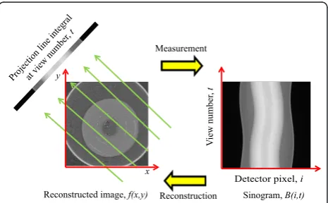
Tomography is the study of the reconstruction of 2D and 3D objects from 1D projections. The projection of an object at a given viewing direction is made up of a set of line integrals. To construct the sinogram, similar projections from a number of viewing directions is obtained and stacked together. In X-ray CT, the line integral represents the total attenuation of the beam of X-rays as it travels in a straight line through the object. As mentioned above, the resulting image is a 2D (or 3D) model of the attenuation coefficient, which is

com-monly known as sinogram B(i, t). Here i denotes the

detector pixel andtdenotes the view number. From this

sinogram, the actual 2D image,f(x,y) is reconstructed

using an appropriate reconstruction algorithm. Figure 1 gives the schematic representation of this procedure.

Measurement

Reconstruction

Projection line integral at view number , t

Reconstructed image, f(x,y) x y

Detector pixel, i

V

iew number

,

t

Sinogram, B(i,t)

R i

In this section, the detection, classification, and cor-rection methods of ring artifacts are discussed in detail. The first two levels of our detection algorithm detect the isolated rings and band rings. The third level of detection detects the residual stripes of the corrected sinogram. Statistical properties of the response of stripe artifacts are used to categorize them into three classes: a) artifacts due to damaged cells and/or damaged scintil-lator and/or dust (Type 1), b) artifacts due to mis-cali-brated detector pixel having time independent beam intensity (Type 2), and c) artifacts due to mis-calibrated detector pixel having time dependent beam intensity (Type 3). The correction method proposed here are exemplar based inpainting algorithm for Type 1 artifact, DC shift for Type 2 artifact and interpolation for Type 3 artifact. The whole ring removal algorithm presented here works in a specific order. The steps of the pro-posed algorithm is given in Table 1.

2.1 Detection of ring artifacts

In sinogram domain, there are stripe artifacts of varying properties. Different types of fault in detector element as described above cause different types of isolated and contagious stripe artifacts. To detect all these artifacts accurately, a three step detection scheme is developed. In the first step, only the most prominent rings are detected around which the band rings occur. In the sec-ond step, the minor rings and the band rings are detected. The third step of detection algorithm works as a feedback step. It checks whether there remains any ring artifact after applying the correction algorithm. If such artifacts are identified, the correction algorithm is applied again on those artifacts. This process continues until all the artifacts are corrected. The three step detec-tion algorithm is described in the following subsecdetec-tions.

2.1.1 First level detection of ring artifacts

In the first level detection of ring artifacts, the difference curve of the corrupted sinogram is exploited. The sum of squared difference curve d(i) of the uncorrected sino-gramB(i,t) is calculated as

d(i) =

t

(B(i,t)−B(i−1,t)) +

t

(B(i,t)−B(i+ 1,t))

2

, (1)

wherei andtare the position of the detector element

and the view number of the sinogram, respectively.

Throughout the entire article, the definitions of iandt

are kept same.

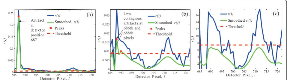
This curve has distinct peaks at the position of faulty detector elements as shown in Figure 2a. These peaks are identified using the first derivative of d(i). Sliding window based data driven threshold is applied to sepa-rate the peaks that are due to the ring artifacts, from the peaks that results from the image detail. This tech-nique is illustrated in Figure 2b. The threshold level changes from window to window. If a constant thresh-old is used for the whole sinogram then it will either fail to detect most of the artifacts or will detect too many false artifacts. In each data window, the threshold level is calculated as

Th = δ

W

i0+W

i=i0

d(i), (2)

whereW is the length of the data window andδis a

constant. In the first level, we are aiming for the detect-ing only the prominent rdetect-ings in the image (large peaks in thed(i) curve), which usually act as the center of the band rings. In the second level of detection, iterative search around these detected ring positions are carried out to detect the adjacent band rings. To detect only the large peaks in the d(i) curve, the threshold levelTh

is set quite high by choosingδ= 8. It has been chosen

by a rule of thumb, and experimentation on a set of real

images has revealed that this is a suitable value ofδat

this level and it does not need any tuning for applying to different types of images. In this study, a total of 13 2D micro-CT images and a single 3D cone beam volume CT image were used. Among the 2D test images there were four synthetic images, seven physiological images and two structural images (like capacitor). The 3D image was a physiological image of a rat abdomen.

The effect of changing δon the reconstructed image is

shown in Figure 3. Here the cow-bone image is chosen as the test image. From the figure it can be observed

that setting δa higher value than 8, results in poor

per-formance because a too high threshold misses the stripes around which band rings may occur. So, even if

Table 1 Steps of ring removal algorithm

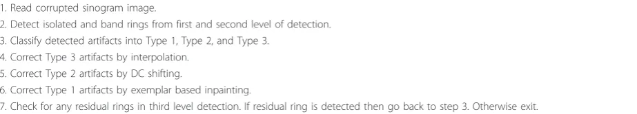
1. Read corrupted sinogram image.

2. Detect isolated and band rings from first and second level of detection. 3. Classify detected artifacts into Type 1, Type 2, and Type 3.

4. Correct Type 3 artifacts by interpolation. 5. Correct Type 2 artifacts by DC shifting.

6. Correct Type 1 artifacts by exemplar based inpainting.

the stripes are detected in the next step, no iterative search is carried out around those, therefore the band rings are remained undetected (see Figure 3e). Again

when δ is set to a lower value then false rings are

detected and processed increasing discrepancies in the image. This phenomena is illustrated in Figure 3d. But

the output image obtained by usingδ= 8 gives the best

result as shown in Figure 3c.

2.1.2 Second level detection of ring artifacts

It is well known that the mean curve of the corrupted sinogram shows peaks at the positions of the faulty

detector element. The mean curve m(i) of the

uncor-rected sinogramB(i,t) is calculated as

m(i) = 1

Ni

t

B(i,t), (3)

where Ni is the total number of detector elements.

Distinct peaks in the mean curve identify defective detector elements. To locate these peaks, at first the

baseline of the mean curvem(i) is estimated by using

the least squares smoothing filter which is more

commonly known as Savitzky-Golay smoothing filter

[16]. The estimated baseline is denoted asz(i). Then the baseline subtracted mean curver(i) is obtained as

r(i) =m(i)−z(i). (4)

The same peak detection and threshold calculation technique, as used in the first level of detection, are applied onr(i). Here the value of the parameterδis set to 2, a lower value than that was set at the preceding level of detection, to enable detection of the minor arti-facts in this phase. But lowering the threshold level leads to detection of some false artifacts. Therefore to

avoid the detection of such false artifacts, r(i) is

smoothed. This reduces the number of trivial peaks inr

(i) which are responsible for false artifact detection. To

smooth r(i), minimax estimation via wavelet shrinkage

technique is used [17]. This technique is particularly suitable in peak preserving noise reduction. The value of

the parameterδat different levels of detection are

vali-dated by experimenting on a number of different types of images and it does not need to be varied from one image to another. The test images that are provided in the results section are all corrected beautifully using these parameter values, giving a proof of the experimen-tal validation.

The second step of the detection process is iterative. After the first iteration, the ring artifacts detected in the first level of detection are made zero. Therefore, the adjacent artifacts are detected as peaks in the next itera-tion. The same process continues iteratively until all the contagious artifacts are detected. This technique is illu-strated in Figure 4.

ROI

(a) (b) (c) (d) (e)

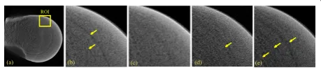
Figure 3Effect of changingδon output image (C/W=.6523/ .7564).(a)Original Cow-bone image,(b)zoomed view of ROI, Zoomed view of output image with(c)_δ= 8,(d)_δ= 5, and(e)_δ= 12. Rings are marked by arrows.

200

400

600

800

1000 1200

0

1

2

3

4

5

6

x 10

Detector Pixel,

i

d(

i)

600

650

700

0

1

2

3

4

5

6

x 10

Detector Pixel,

i

d(

i)

T

Da ta

Wi ndow

Da ta

Wi ndow

(a)

(b)

2.1.3 Third level detection of ring artifacts

After application of the correction algorithm, some minor residual artifacts may still remain. Such a case is illustrated in Figure 5. There is a very minor artifact at the detector position 627 (see Figure 5a). Its response resembles the response of adjacent non-defective pixels

and also the shift from the non-defective pixels’

responses is very negligible (see Figure 5b). Therefore, these artifacts will not show distinct peaks ind(i) orr(i). A simple algorithm is considered for detecting these minor artifacts. It is observed that generally the response of a good pixel lies in between the nearmost preceding and succeeding non-defective pixel whereas faulty

detec-tor pixel’s response will either lie above or below of

both the non-defective responses. As can be observed from Figure 5b, the response of the faulty pixel at 627 lies above of the two adjacent non-defective responses. This property is used here to detect these artifacts. An interesting feature of this technique is that rather than calculating the amplitude difference between the adja-cent defective and non-defective element (which is very low), it counts the number of points of the response curve of a faulty detector in which the amplitude of intensity is not in between the near most preceding

defective detector element and succeeding non-defective detector element. The total number of such

points in a response of detector position iis denoted as

c(i). Ifc(i) is plotted against the detector position then the detector elements causing minor artifacts show dis-tinctly higher values than that of non-defective detector elements as shown in Figure 5c. Then by applying a sui-table threshold on c(i) these artifacts can be identified.

The threshold levelTc is estimated from the mean of

this curve.

This residual ring artifact detection technique is a new feature. In no other reported work in this field has pro-posed any technique for detecting such residual rings. This detection step enhances the performance of the total ring removal algorithm significantly. In addition to that, the iterative band ring detection method proposed here is also a novel concept compared to other reported band ring detection schemes, e.g., polyphase decomposi-tion of sinogram [15].

2.2 Classification of ring artifacts

After detecting the ring artifacts, they are categorized into three different types. From a careful observation of

620 622 624 626 628 630 632 50 100 150 200 250 300 350 400 Minor ar ti fact at det ect or pixeli= 627

200 400 600 800 1000 1200 0 50 100 150 200 250 300 350 400

Det ector P ixel,i

c(

i)

Tc Artifact

at det ector pixel,i= 627

220 240 260 280 300 320 340

0.82 0.84 0.86 0.88 0.9 0.92 0.94 0.96 0.98

View Number ,t

In

te

n

sit

y

626t h p ixel

627t h p ixel (faulty )

628t h p ixel

Det ector P ixel,i

V iew N u m ber , t

(a) (b) (c)

Figure 5Minor artifact detection.(a)Minor artifact in sinogram domain at detector celli =627,(b)response of artifact creating cell ati =627 along with the responses of surrounding non-faulty detector cells, and(c)detection of artifact ati =627.

685 690 695 700 705 710 715 720 0 0.05 0.1 0.15 0.2 0.25

Detector P ixel,i

r( i) r(i) Smoothed r(i) Peaks Threshold Arti fact at dete ct or positi on 687

685 690 695 700 705 710 715 720 0 0.005 0.01 0.015 0.02 0.025 0.03

Detector P ixel,i

r( i) r(i) Smoothedr(i) Peaks Threshold Two contagiou s ar ti fact s at 686t h and 688t h pixels

685 690 695 700 705 710 715 720 2 4 6 8 10 12 14 16

Det ector P ixel,i

r

(

i)

r(i) Smoothedr (i)

Threshold

(a) (b) (c)

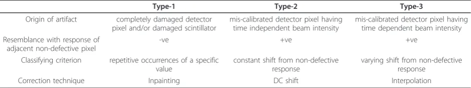
responses from different types of faults in a sinogram, it is found that the responses of defected cells (a) may or may not follow the overall pattern of response of the adjacent non-defective cells, (b) follow the response of non-defected cell with a constant or varying shift, and (c) exhibit repetitive occurrence of a certain value in the response of the fault. All these phenomena that are used to classify different types of faults in a corrupted

sino-gram are summarized in Table 2, where ‘+ve’and‘-ve’

terms are used to mean whether the specific criteria is present or not in a certain type of artifact. If the criteria is present in a type of artifact,‘+ve’is entered in the col-umn of that type and vice versa. Different types of faults are described below.

2.2.1 Type 1 artifact

Artifacts of Type 1 occur due to completely dead cells of the detector panel and/or damaged scintillator. It does not follow the pattern of adjacent non-defective cell at all. Moreover, in the response of this type of fault repetitive occurrences of a particular value is observed. An example of the response of this type of artifact is given in Figure 6a. The value that has the highest occur-rence in an array is defined as the mode of the array.

Let the response of a defective detector at the ith

posi-tion is denoted asxi(t). At first the mode mdof xi(t) is determined. Let us define a set Ci={xi(t)|xi(t) =md},

which contains values of xi(t) equal to modemdfor the ith detector position. Then cm(i) =|Ci| denotes how

many times the mode has occurred in the detector cell response. Since the property of repetitive occurrence of a specific value is present only in Type 1 artifacts,cm(i) of Type 1 faults will have much higher value than the other two types of artifacts. This is illustrated in Figure 6c. Then, from this curve artifacts of Type 1 are easily classified by using a simple thresholding technique. The

threshold Tcm for separating Type 1 artifacts from Type

2 and Type 3 artifacts is calculated as

Tcm = δ Nf

Nf

i=1

cm(i), (5)

where Nfis the total number of faulty detector cells

present in the sinogram, and the value for the parameter

δis chosen to be the same as that in the second level of

detection.

The classification criterion proposed here is a new one. This type of artifact was also classified in [15]. But the classification technique was different. For classifica-tion, at first the non causal first derivative of the sino-gram was computed. Then the difference array was calculated by taking the sum of derivative value along each detector pixel. The criteria for separating the arti-facts due to the dead pixels from the artiarti-facts due to the mis-calibrated pixels was based on this array. Generally, Type 1 artifacts show higher value in the array than the artifacts due to the calibrated pixels. But if the mis-calibrated pixel has a high amplitude shift from the adjacent good pixels, then it will also have a high value in the difference array and hence can be classified as Type 1 artifact. Therefore, the classification technique proposed in [15] may not be robust in such cases. But in the proposed technique here, the classification criter-ion is derived from the statistical property of the response of faulty pixels. The most significant statistical properties which are exclusive for each type of fault are proposed here as classification criteria. Therefore, it can be inferred that the proposed classification scheme will be more robust in categorizing faults in a corrupted sinogram.

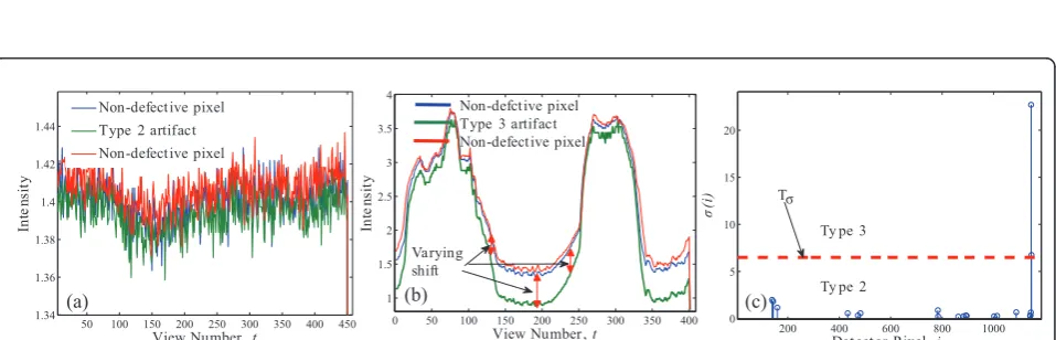
2.2.2 Type 2 artifact

Type 2 artifact occurs due to the mis-calibrated detector elements having time independent X-ray beam intensity. It has no repetitive occurrence of a particular value in the response of the mis-calibrated detector element. It follows the response of the adjacent non-defective cell but with an amplitude shift of almost constant value. Response of this type of artifact is illustrated in Figure 7a.

2.2.3 Type 3 artifact

Type 3 fault may occur due to mis-calibrated detector element having time dependent X-ray beam intensity. It also does not have repetitive occurrence of a particular value in the responses of the detector elements. It fol-lows the pattern of the response of adjacent non-defec-tive cells but the amount of shift from the response of non-defective cells varies greatly from one point to another (see Figure 7b).

Table 2 Different types of artifacts

Type-1 Type-2 Type-3

Origin of artifact completely damaged detector pixel and/or damaged scintillator

mis-calibrated detector pixel having time independent beam intensity

mis-calibrated detector pixel having time dependent beam intensity Resemblance with response of

adjacent non-defective pixel

-ve +ve +ve

Classifying criterion repetitive occurrences of a specific value

constant shift from non-defective response

varying shift from non-defective response

To classify artifacts of Type 2 and Type 3, an array is calculated by taking the point to point difference between the baselines of the adjacent defective and non-defective cells. Their baseline estimation is the same as that of the mean curve described earlier in the second level detection of artifact. We definez1(t) as the baseline

of the response curve of a faulty detector cell at position

i andz2(t) as the baseline of its adjacent non-defective

cell. The point to point difference array for faulty detec-tor at positioni is then denoted byli(t). Then li(t) is

normalized and the standard deviationsof the

normal-ized array is calculated. Mathematically,

λi(t) =z1(t)−z2(t), (6)

λni(t) = 1

max(λi(t))λ

i(t), (7)

σ =

1

N

t

(λni(t)−μ)

2

. (8)

Here λni(t) denotes the normalized value ofli(t) and

μis the mean of λni(t). Thussfor all the faulty

detec-tor cells except Type 1 are calculated and plotted against the detector cell position. Since the response of Type 3 artifact has varying shift from the adjacent non-defective cell’s response,sof this type of fault will defi-nitely have higher value than that of Type 2. This is

illu-strated in Figure 7c. The threshold level,T_sto separate

Type 3 artifacts from Type 2 is calculated in the same way as in classification of Type 1. Ifcm(i) is replaced by

s(i) andNfis replaced by Nf23 thenTscan be calculated

using (5). Here Nf23 = total number of Type 2 and Type

3 artifacts in the sinogram. The detected pixels that

100 200 300 400

0 0.5 1 1.5 2 2.5 3

View Number ,

t

In

te

n

si

ty

Good pixel Defect ive pixel Good pixel

200 400 600 800 1000

0 50 100 150 200

Detector Pixel,

i

c

(i

)

Type 2 and Type 3 Type 1 Tcm

(a) _(b)

Figure 6Type 1 fault.(a)Response of a completely damaged detector cell and(b)separation of Type 1 artifacts from Type 2 and Type 3 artifacts.

50 100 150 200 250 300 350 400 450 1.34

1.36 1.38 1.4 1.42 1.44

View Number ,t

In

te

n

sit

y

Non-defect ive pixel

Type 2 artifact

Non-defect ive pixel

0 50 100 150 200 250 300 350 400 1

1.5 2 2.5 3 3.5 4

View Number ,t

In

te

n

sit

y

Varying shift

Non-defct ive pixel Type 3 artifact Non-defect ive pixel

200 400 600 800 1000

0 5 10 15 20

Det ect or P ixel,i

σ(

i)

Ty pe 2 T

Ty pe 3 σ

(a) (b) (c)

have theirshigher thanTsare classified as Type 3

arti-facts and the rest are grouped as Type 2 artiarti-facts.

2.3 Correction of ring artifacts

While correcting the artifacts from the corrupted sino-gram, Type 2 and Type 3 artifacts are required to be corrected first. The inpainting algorithm employed to correct Type 1 artifact divides the sinogram into two regions. The Type 1 artifacts are defined as the target region and the rest of the image is defined as the source region. This algorithm takes information from the source region to fill in the target region. For effective implementation of the inpainting algorithm, the source region is needed to be artifact free. For this purpose, Type 3 and Type 2 artifacts are corrected first to pro-vide an artifact free source region. Detailed description of the correction techniques is presented in the following.

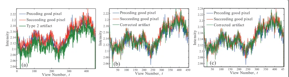
2.3.1 Correction algorithm for Type 3 artifact

To correct this type of artifact interpolation technique is used. In this type of artifact, defective response is quite similar to that of a non-defective one. As it contains some of the image information, complete reconstruction

by computationally cumbersome techniques like inpaint-ing is not desired here. DC shiftinpaint-ing is not appropriate either because a deviation from the response by different value at different points is not unlikely. Therefore, a constant shifting will not remove artifacts of this type rather there is a probability that it will introduce new ring. Considering all these facts, interpolation technique is proposed here for correcting artifacts of this type. At first the positions of near most preceding and succeed-ing non-defective detector cells are found. Then ussucceed-ing the responses of these two non-defective detector cells, the response of the Type 3 artifact in between them is interpolated. Spline interpolation technique is used for this purpose.

Identification of Type 3 artifact and proposing a sepa-rate correction technique suitable for this type of artifact is a major novelty of this work. In [15], Type 2 and Type 3 artifacts were not separately addressed. They were grouped under the category of mis-calibrated arti-facts and the normalization technique was used for

cor-recting both these types of artifacts. In the

normalization technique, every point on the defective response curve is scaled by a fixed value. As can be

50 100 150 200 250 300 350 400 45 2.06 2.08 2.1 2.12 2.14 2.16 2.18 2.2 2.22 2.24

View Number ,t

In

te

n

sit

y

Preceding good pixel Succeeding good p ixel Corr ected ar tifact

0 100 200 300 400

2.04 2.06 2.08 2.1 2.12 2.14 2.16 2.18 2.2 2.22

View Number ,t

In

te

n

sit

y

Preceding good pixel Succeeding good p ixel Ty pe 2 artifact

50 100 150 200 250 300 350 400 450 2.06 2.08 2.1 2.12 2.14 2.16 2.18 2.2 2.22

View Number ,t

In

te

n

sit

y

Preceding good pixel Succeeding good p ixel Corr ect ed ar tifact

(a) (b) (c)

Figure 9Correction of Type 2 artifact.(a)Response curve of Type 2 artifact,(b)corrected response by the normalization technique, and(c) corrected response by the proposed DC shift technique.

0 50 100 150 200 250 300 350 400 1 1.5 2 2.5 3 3.5 4

View Number ,t

In

te

n

sit

y Preceding good pixel

Succeeding good p ixel Type 3 art ifact

50 100 150 200 250 300 350 400 0.5 1 1.5 2 2.5 3 3.5 4

View Number ,t

In

te

n

sit

y

Preceding good pixel

Succeeding good p ixel

Corr ect ed ar tifa ct

50 100 150 200 250 300 350 400 1 1.5 2 2.5 3 3.5

View Number ,t

In

te

n

sit

y

Preceding good pixel

Succeeding good p ixel

Corr ected ar tifa ct

(a) _{(b) (c)}

observed from Figure 8, that a fixed scaling for every point of the defective response will not remove this type of artifact. Figure 8b,c illustrate the performance of the normalization technique and the proposed interpolation technique on the response curve of a Type 3 artifact. The normalization technique completely fails to correct the response curve. Moreover, it creates new discrepan-cies in some regions (see Figure 8b). Whereas the pro-posed interpolation technique here corrects the faulty response curve perfectly (see Figure 8c). Therefore, the proposed technique definitely outperforms the normali-zation technique and hence emphasizes the need of categorizing these artifacts as a separate class and apply-ing separate correction technique for this type.

2.3.2 Correction algorithm for Type 2 artifact

DC shifting technique is used to correct this type of fault. Since in this case, the response of the faulty detec-tor element shifts from the response of the adjacent good detector by almost a constant value, therefore if the response of the faulty detector element can be shifted by that value then this type of fault can be cor-rected. Assume that there is a Type 2 artifact at the

detector position iof the sinogram B(i,t). The amount

of shift necessary to correct the fault is calculated from

β(i) = 1

2Nt

t

B(i,t)−B(i−k1,t)+

t

B(i,t)−B(i+k2,t)

, (9)

where (i -k1) and (i+k2) are the indices of nearmost

preceding non-defective cell and succeeding

non-defec-tive cell, respecnon-defec-tively.tis the index of view number and

Ntis the total view number. k1 andk2are preceding and

succeeding lag parameters, respectively. In case of iso-lated artifact,k1 =k2 = 1 and in case of contagious

arti-facts {k1, k2} > 1 depending on the width of the band

ring. If the mean value of the faulty pixel responsexi(t) is higher than that of both the adjacent preceding and

succeeding non-defective pixels’responses then the

cor-rected response xi˜(t) is calculated as

˜

xi(t) =xi(t)−β(i). (10)

In all other cases,

˜

xi(t) =xi(t) +β(i). (11)

Here a new technique is used to calculate the DC shift of the faulty detector. In [15], the normalization techni-que was used to correct this type of artifacts. Normaliza-tion technique works good on Type 2 artifacts but the success of this technique depends greatly on the estima-tion of corrected mean curve. Whereas our proposed technique is free from such dependency. It calculates the shift directly from the original sinogram. The perfor-mance of the proposed method and the normalization method on Type 2 artifact is shown in Figure 9. Both the techniques remove the artifact quite satisfactorily.

2.3.3 Correction algorithm for Type 1 artifact

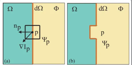
Exemplar based image inpainting technique [18] is applied here to correct faults of Type 1. The whole

sino-gram I is divided into source region (F) and target

region (Ω) (see Figure 10). The contour of the target

region isδΩ. At first, this algorithm determines a filling order. For this purpose, priorities of the patches (tem-plate windows (Ψp) of size 9 × 9 pixels) on the fill front

are calculated. In general words, the patch Ψpthat has

most of the pixels already in the source region and very few on the target region has high priority. In this

algo-rithm, every pixel has a colorvalue and a confidence

value. A pixel has a high confidence value if it is a part of the source region or it is in the target region but already filled by the algorithm.

Given a patch Ψpcentered at the point p Î δΩ, its

priorityP(p) is defined as

P(p) =C(p)D(p), (12)

d

Ω

p

p

Ψ

Ω

Φ

p

p

n

I

Δ

p

d

Ω

Ψ

Ω

Φ

p

p

(a) (b)

Figure 10Notation diagram for the inpainting algorithm.(a) Given the patchΨp,npis the normal to the contourδΩof the

target region_Ωand_∇Ipis the isophote (direction and intensity) at

pointp;(b)after first iteration of the algorithm, the target region_Ω has shrank and its contour_δΩhas moved deeper into it.

Table 3 Inpainting algorithm

1. Identify the target regionΩfrom the ring location of Type 1. 2. Set the iteration indexk= 0.

3. Identify the fill frontδΩk_{, i.e., contour of the target regionΩ}k_.

4. Compute prioritiesP(p) forΨpÎδΩ k

.

5. Find the patchΨpwith maximum priority, i.e., for

p= arg maxp∈δkP(p)

6. Find the exemplarΨqÎ Fthat minimizesd(Ψp,Ψq).

7. Copy the image data fromΨqtoΨp.

8. UpdateC(p).

9. Increasekby 1 for next iteration.

10. Check whetherFk_{=j. If yes then exit. Otherwise go back to step}

whereC(p) is the confidence term andD(p) is the data term, which are defined as

C(p) = q∈p∩C(q)

p

, (13)

and

D(p) = ∇Ip.np

α , (14)

where |Ψp| is the area of Ψp,a is the normalization

factor (e.g.,a =255 for a typical gray level image), (.) is

the dot product operator, and npis a unit vector

ortho-gonal to the fill front δΩat the point p. All notations

are shown in Figure 10. For initialization, the functionC

(p) is set toC(p) = 0 forΨpÎ ΩandC(p) = 1 forΨpÎ

(I- Ω). After determining the fill order, the patch with

the highest priority is filled with values extracted from the source region. The patch in the source region which

is the most similar toΨpis defined as the best exemplar

patch. The best exemplar patchΨq is obtained from

q= arg min

q∈φ d(p,q), (15)

where the distanced(Ψp,Ψq) between the two patches

Ψpand Ψq is defined as the sum of the squared

differ-ences of the filled pixels in the two patches. Having

found the source exemplar Ψq, the value of each pixel

to be filled pÎ (Ψp∩F) is copied from its

correspond-ing position insideΨq.

After the patchΨphas been filled with the new pixel

values, the confidence valueC(p) is updated as

C(q) =C(p),q∈(p∩). (16)

The whole inpainting algorithm as in [18] is given here in Table 3.

To make this algorithm applicable to ring artifact cor-rection, the entire sinogram image is divided into source and target region. All stripes of the artifact correspond-ing to Type 1 faults are replaced with a constant value higher than the maximum value of the sinogram so that these stripes can be identified by the algorithm as the target region. This algorithm requires a specific color value of the target region as an identifier. Therefore, the image is first converted into an indexed image and then to a RGB image. The stripe artifacts replaced with a

constant value are defined as the target region Ω and

the rest of the image as the source regionF.

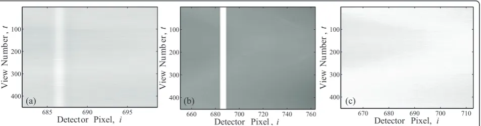
Implemen-tation of this technique on the sinogram is shown in Figure 11.

The application of exemplar based inpainting in removing stripe artifacts is a new approach. The more general convolutional approach of image inpainting is in particular not suitable for removing the wide band rings.

Detector Pixel, i

View

Nu

m

b

er

,

t

685 690 695

100

200

300

400

Detector Pixel ,i

View

Nu

m

b

er

,

t

660 680 700 720 740 760

100

200

300

400

Detector Pixel, i

View

Nu

m

b

er

,

t

670 680 690 700 710

100

200

300

400

(a) (b) (c)

Figure 11Correction of Type 1 faults.(a)Type 1 artifact in sinogram domain,(b)stripe artifact replaced by a constant value, and(c) corrected sinogram after inpainting.

ROI

(a)

(b)

(c)

(d)

(e)

In such a case, the band ring will occupy most pixels in the convolution window and as a result the source information in the window will be reduced. Therefore the inpainting of the target region may not be robust. If the convolution window size is increased then there is a possibility that the target region will be inpainted with the values that are not relevant to it. Then the perfor-mance of the inpainting algorithm may not be satisfac-tory. But in the proposed inpainting technique instead of convolution, the target region is filled by values that are most relevant to it (i.e., by finding the best exemplar patch). Therefore, blurring effect is more unlikely in this algorithm. The proposed algorithm is also insensitive to the patch window size. The effect of changing the patch window size on output image is illustrated in Figure 12. Here three different window size is implemented and in all cases the image is corrected quite effectively irrespec-tive of the window size which consequently proves the robustness of the algorithm.

3 Result and analysis

The test images were acquired with a home made micro-CT which consists of a CMOS FPD and a micro focus X-ray tube (L8121 - 01, Hamamatsu, Japan). The micro-focus X-ray source is a sealed tube with a fixed tungsten anode having an angle of 25° against the

elec-tron beam and with a 200 μm-thick beryllium exit

win-dow. The emitted X-ray beam span angle is about 43°.

The source has a variable focal spot size from 5μm to

50 μm depending on the applied tube power (Watt or

kVp mA). The maximum tube voltage and tube current are 150 kVp and 0.5 mA, respectively. The micro-focus X-ray source has been operated in a continuous mode with an Al filter with a thickness of 1 mm. The FPD (C7943CA-02, Hamamatsu, Japan) used in this experi-ment consists of 1216 × 1220 effective matrix of

transis-tors, photodiodes with a pixel pitch of 100 μm and a

CsI:Tl scintillator. The CsI:Tl has a columnar structure

with a typical diameter of about 10 μm and a thickness

of 200μm. A computer-controlled rotating system was

adopted in the object holder to achieve a cone-beam mode scan in the micro-CT. The precision of the rota-tional motion is 0.083° which allows the number of views larger than 4,000. The system has the built-in white and dark image correction schemes. Since our micro-CT system does not provide the CT images in Hounsfield unit (HU), we have normalized all the origi-nal (uncorrected) reconstructed images so that the max-imum pixel intensity is 1.0 with arbitrary unit. The corrected images are scaled using the corresponding normalization factor of the uncorrected images.

The performance of the proposed algorithm is com-pared with two recently reported ring removal algo-rithms [11,15]. The reported algorithm in [15] classifies

strong artifacts due to dead pixels and weak artifacts due to mis-calibrated pixels and proposes 2D variable window moving average (2D VWMA) and 2D weighted moving average (2D WMA) filter for correcting the strong rings and normalization technique for correcting the mis-calibrated artifacts. The mis-calibrated artifacts due to time dependency of beam intensity were not separately classified and hence no algorithm was pro-posed for correcting this type of artifact. There are four adjusting parameters in that algorithm (rmax,rmin, lm,a)

which are required to be set manually. rmaxandrminare

suitably defined upper and lower threshold for detection

and classification of ring artifacts.lmis the number of

levels of polyphase decomposition of the sinogram image. Polyphase decomposition is used in the reported

work to detect the band ring.ais a constant used in the

equation of detection algorithm of the ring removal technique [15]. These parameter values are required to be changed from one image to another for obtaining the best result. But in the ring removal algorithm proposed in this article, the data driven thresholding technique is automatic and performs satisfactorily on all the test CT images. The rigorous classification scheme presented here discovers a new class of artifact in CT image (Type 3). Since three separate correction techniques are pro-posed here for the three types of artifacts, the overall performance of the correction algorithm is certainly improved. Our proposed algorithm and the algorithm presented in [15], both works in the sinogram domain.

To compare the performance of our sinogram proces-sing technique with post procesproces-sing techniques of ring removal, a reported algorithm [11], which works in the reconstructed image domain is also considered. This algorithm applies mean and median filtering technique to remove ring artifacts but it works in a different geo-metrical plane (in polar coordinate). The filter width of the ring correction in polar coordinate (RCP) method [10] is selected as suggested in the original work, e.g., radial median filter width in polar coordinates,

MP

Rad= 15; azimuthal filtering in polar coordinates,

MP

AZi= 40. On the other hand, the distance between the

support points in the azimuthal direction (dP

AZ) for the

polar coordinate is needed to be adjusted for our test

CT images. We set dP

AZ equal to 0.7°, instead of 0.8°. In

the original work [10], the distance between the support points in the radial direction (dRA) for both the cartesian

and the polar coordinates is determined from the scan-ner geometry. In our case, this parameter is set to 1.0

for the polar coordinate (dP

RA). The RCP method uses

three thresholds (Tmin, Tmax, and TRA) for image

work. As in this work, the CT images are not calibrated in HU unit, therefore, these thresholds should be selected in such a way that the purpose of these

thresh-olds is served. The lower (Tmin) and upper (Tmax)

thresholds are set to the minimum and maximum values of the ring intensities found in the CT image, respec-tively. As a result, the image elements having intensities above or below the ring artifact intensities are not affected by the correction algorithm. Similarly, the third

threshold (TRA) is set to the maximum value of ring

intensities in the difference image obtained after median filtering. The main draw back of the RCP method is its failure to remove strong rings with varying intensities. Because, they generally contain significant high fre-quency information but the mean (low-pass) filtering in the RCP method is not appropriate to retain the correct varying intensity ring structures in the difference image and thereby may result in poor performance of the algo-rithm. In addition to that, this algorithm does not pro-vide any classification scheme for the artifacts present in a CT image.

For quantitative performance evaluation, we have used two numerical indices. One is the peak signal-to-noise ratio (PSNR) and the other is the mean struc-tural similarity (MSSIM) [19]. The PSNR is related to the intensity difference between the reference and the corrected images. The second index, MSSIM can be correlated to the perceptual quality of an image. It considers luminance, contrast and structure similarity between the reference and corrected images to deter-mine the value of the index. But evaluation of these two indices requires reference images, i.e., images free from ring and radiant artifacts. In CT imaging refer-ence image is hardly available and, therefore, in this work three synthetic (computer simulated phantom) sinogram images have been used. Different types of stripe structures discussed in this article including sin-gle, band, stripes from defective and mis-calibrated detector elements are superimposed on the reference sinogram images to generate corrupted sinogram images. The proposed technique and the sinogram-processing technique in [15] are applied on these cor-rupted sinogram images and the post-processing tech-nique [11], on the other hand, is applied on the CT images reconstructed from the corrupted sinograms. Now the above mentioned two indices can be calcu-lated to quantify the visibility of errors between the reference and corrected CT images. The first quantita-tive index PSNR is defined as

PSNR = 20log₁₀

M

√

MSE

dB (17)

where,

MSE = 1

PQ

P−1

i=0

Q−1

j=0

[X(i,j)−Y(i,j)]2 (18)

whereX|PQand Y|PQare the reference and corrected

CT images, respectively and,MIis the dynamic range of

the reference image.

To calculate the MSSIM index at first the reference and corrected CT images are windowed and two signals, i.e., x(x= [x1x2 ...xN]) and y(y = [y1y2 ...yN]) are gener-ated in each window. Then these two signals are

weighted using a Gaussian weighting function, w =

[w1w2 ... wN] with a standard deviation of 1.5 samples,

whereΣi=1wi = 1. Then in each window, the estimates

of local statistics ofxandyare calculated as:

μx=

1

N N

i=1

wixi (19)

μy=

1

N N

i=1

wiyi (20)

σx=

1

N−1

N

i=1

wi(xi−μx)2 (21)

σy=

1

N−1

N

i=1

wi(yi−μy)2 (22)

σxy=

1

N−1

N

i=1

wi(xi−μx)(yi−μy) (23)

The SSIM index between signalsx(x= [x1x2...xN]) and y(y= [y1y2...yN]) in each window is calculated as [19]

SSIM = (2μxμy+C1)(2σxy+C2)

(μ2

x+μ2y +C1)(μ2x+μ2y +C2) (24)

where,C1 = (K1 MI)2, C2 = (K2MI)2,K1= 0.01, and K2

= 0.03. Finally, the mean SSIM (MSSIM) is evaluated as

MSSIM = 1

M M

j=1

SSIMj (25)

where, SSIMjis the SSIM calculated at the jth local

window and M is the number of local windows in the

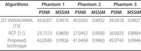
The calculated PSNR and MSSIM values for the three simulated phantom images are shown in Table 4. As can be observed from the table, the overall performance of the proposed technique is better than the 2D VWMA/WMA method on the simulated phantom images. On the other hand, the performance of the post processing based RCP technique is not found very impressive on the simulated phantom images, which is reflected in the lower MSSIM and PSNR values.

Next, to compare the performance of our proposed algorithm with the two reported techniques [11,15], a test image is chosen which has all the three types of artifacts. The image of Rabbit-femur is an ideal example of such an image (see Figure 13). The corrected images obtained by the reported techniques and by our pro-posed technique is illustrated in Figure 13b-d. As can be observed from Figure 13b, the ring removal algorithm presented in [15] fails to correct all the artifacts in the image. The Type 3 artifacts near the center of the image remain uncorrected. The reason behind the failure of the algorithm in correcting Type 3 artifact is explained earlier in the section of Type 3 artifact correction. The 2D VWMA/WMA technique works satisfactorily on the outer ring of Type 1. The values of tunable parameters are chosen as {rmax,rmin,lm,a} = {20, 2, 4, 1} for obtain-ing the optimum results. On the other hand, in the cor-rected image obtained by the technique presented in [11] is still corrupted with a number of residual rings (see Figure 13c). In addition to that, the radial artifacts are also persistent in the corrected image. But, the pro-posed technique here removes all the artifacts beauti-fully to produce a ring free image (see Figure 13d). The elegant detection and classification scheme and the application of customized correction algorithm for each type of artifact ensure the best result. The experimental results on the Rabbit-femur image thus demonstrate the efficacy of the detection, classification and correction scheme proposed in this article.

The proposed ring removal technique corrects rings without introducing visible distortion in the image. To show this, test images of a Capacitor and a Rat-chest are chosen (see Figure 14). The Capacitor image is an example of highly structural object (see Figure 14a).

This image shows a number of fabrication layers in the capacitor. There is a strong ring in one of these fabrica-tion layers. To observe the hidden micro-structure of the image this ring is required to be corrected without impairing the visual quality of the image detail. From Figure 14b, it can be seen that the proposed correction technique applied on Capacitor image, neither obscures nor distorts the structural details of the image. So, it can be inferred that in preserving structural details of the CT image, the performance of the algorithm is satis-factory enough. Small animal imaging is an important field of CT imaging. The Rat-chest image is an example of small animal imaging. This image has very fine phy-siological details (see Figure 14c). The corrected image in Figure 14d obtained by the proposed algorithm illus-trates that there is no distortion in the fine physiological details of the image while all the ring artifacts are removed successfully. This proves the effectiveness of our algorithm in small animal imaging.

To prove the accuracy of the proposed algorithm, another special case is considered. When a high contrast circular object is placed at the center of rotation of the CT image, it appears as a band of stripes in the sino-gram domain. These stripes are part of image detail and hence should not be corrected. Such a case is illustrated in Figure 15. A thin gold wire is placed at the center of rotation. The position of the gold wire in the uniform phantom is marked by arrow in Figure 15a,b and as a result, a band of stripes having width of 9 pixels (pixels 1159-1167 as shown in Figure 15e) is generated in the sinogram (marked by arrow in Figure 15d). Since the proposed ring removal technique is based on correcting stripes from the sinogram domain, there is a probability that it will identify the stripes as ring artifacts and hence may correct them. But interestingly using the proposed method, only a single pixel of the 9 pixels band is detected as artifact and has undergone for correction. The corrected image is shown in Figure 15c. The cor-rection of only one pixel does not introduce noticeable distortion of the image. In the first level of detection, this band ring have very small amplitude in the sum

squared difference curve d(i) (marked by red circle in

Figure 15g) and in windowed data driven thresholding technique it is not detected as artifact. But in the second level of detection a single pixel (Pixel 1163) of the band ring is detected from the plot of r(i) and classified as a mis-calibrated artifact (Figure 15h). Since an iterative search is conducted for band rings around only those artifacts that are detected in the first level of detection, therefore the band of stirpes around the 1163th pixel is not detected as band ring. Thus from Figure 15f it is seen that preserving this band of stripes, the algorithm corrects all other ring generating stripes. Therefore, based on the performance of the algorithm in this case

Table 4 Quantitative performance analysis of the ring removal algorithms on simulated phantoms

Algorithms Phantom 1 Phantom 2 Phantom 3

PSNR MSSIM PSNR MSSIM PSNR MSSIM

2D VWMA/WMA [15]

43.6207 0.9910 40.0263 0.9932 39.0318 0.9927

RCP [11] 23.7213 0.8600 27.0452 0.9500 26.0023 0.8904 Proposed

technique

it can be predicted that the proposed technique will be effective in other similar cases, e.g., when there is a small lesion present at or near the iso-center.

3D cone beam volume CT imaging is a new imaging modality. The proposed ring removal algorithm is also applicable for cone beam geometry. Sinogram by sino-gram processing technique is employed to correct such 2D cone beam projection images. At first a sonogram is constructed from the 2D stack of projection data and then the ring removal algorithm is applied to it. The

corrected sinogram is then transferred back into the projection domain and then the next sinogram is read. The process continues until all the 2D projections are corrected. Finally, the FDK algorithm [20] is used to reconstruct the corrected 3D cone beam volume CT image. To demonstrate the effectiveness of the proposed algorithm and to compare its performance on 3D cone beam volume CT images with the 2D VWMA/WMA and RCP techniques, Rat-abdomen image is chosen as an example. The 2D VWMA/WMA method [15], the

(a)

(b)

(c)

(d)

RCP method [11] and the ring removal algorithm pre-sented here are applied to correct three slices taken from different locations. The tunable parameters used in

the 2D VWMA/WMA method, i.e., {rmax, rmin, lm, a}

are kept fixed for correcting each slice of the three slices. To compare the performance of the proposed technique with the two reported techniques, 401th, 601th and 801th slices are chosen from the test image (see Figure 16). The region near the center of rotation is

marked as region of interest (ROI). The original slices and zoomed view of their ROIs are illustrated in the first column of Figure 16. The second, third and fourth column correspond to the corrected slices obtained by the 2D VWMA/WMA [15], the RCP [11], and the pro-posed technique, respectively. The parameter values of

2D VWMA/WMA method are set as {rmax, rmin, lm, a}

= {30, 1, 4, 1}. As can be observed from the second col-umn of Figure 16, that the ring removal technique

(a)

(d)

(b)

(c)

reported in [15] fails to correct the rings near the center of rotation of the image in all the test slices. In addition to that, the algorithm also fails to correct some outer rings from the 601th and 801th slices. Again in case of the RCP technique [11], the corrected slices (see the third column of Figure 16) are distorted by the presence of radial artifacts. Blurring effect is also noticeable here. In addition to that, the ring artifacts are also not

corrected effectively. A number of residual ring artifacts are present in the corrected image. Whereas our pro-posed algorithm removes all the ring artifacts from the three slices of the 3D CT image successfully (see the fourth column of Figure 16). Comparing the corrected images obtained by the two reported techniques with the corrected images obtained by our proposed techni-que, it is quite obvious that the proposed technique

Vi

e

w

N

u

m

b

e

r,

t

500 1000 1500 2000

100

200

300

400

500

600

700

800

900

Vi

e

w

N

u

m

b

e

r,

t

1160 1165 1170

100

200

300

400

500

600

700

800

900

Band of Stripes Pixel−1159−1167

Det ect or P ixel,i

Vi

e

w

N

u

m

b

e

r,

t

500 1000 1500 2000

100

200

300

400

500

600

700

800

900

1140 1150 1160 1170 1180 1190 1200

0 0.5 1 1.5 2

x 105

Det ect or P ixel, i

d(

i) Th

Band of Stripes

1120 1130 1140 1150 1160 1170 1180 1190

0 0.01 0.02 0.03 0.04 0.05 0.06 0.07 0.08

Det ect or P ixel, i

r(

i)

Th

1163th pixel

Det ect or P ixel,i Det ect or P ixel,i

(a)

(g)

(h)

(d)

(e)

(f)

ROI

(b)

(c)

(a)

ROI ROI ROI ROI

ROI

ROI ROI ROI ROI

ROI ROI ROI

(a)

(x) (w)

(v) (u)

(t) (s)

(r) (q)

(m) (n) (o) (p)

(l)

(j) (k)

(h) (d)

(e) (f) (g)

(c) (b)

(i)

here outperforms the reported algorithms convincingly. Therefore, it can be inferred that the proposed algo-rithm is comparatively effective in removing ring arti-facts from 3D cone beam CT images.

4 Conclusions

This article has dealt with an improved ring artifact sup-pression method for FPD based CT images. A rigorous three step detection algorithm has been proposed here. The detection technique exploits both the mean curve and the difference curve to improve accuracy in ring artifact detection. Introduction of a feedback loop for detection is a new feature of the proposed ring removal algorithm. The iterative band ring detection method is also a new approach in detecting contagious artifacts, which is a common phenomena in CT images. A new class of artifacts has been included in the proposed clas-sification scheme. All the threshold levels used in detec-tion and clarificadetec-tion algorithm are data driven and automatic. Separate correction algorithms have been proposed here to correct each type of faults. Therefore, customized correction algorithms ensures the best result in removing ring artifacts from the CT images. The per-formance of the proposed algorithm has been tested and compared with other reported algorithms using both fan beam and cone beam geometry based CT images. To evaluate the performance of the proposed algorithm, some special cases has also been considered, e.g., images with highly structural and physiological details and images with high contrast cylindrical object at the iso-center. The comparative results have revealed that the proposed technique removes the ring more effectively compared to the other two reported techniques in this article.

Acknowledgements

This study was supported in part by the National Research Foundation (NRF) of Korea funded by the Korean government (MEST) (No: 2009-0078310).

Author details

1_{Department of Electrical and Computer Engineering, University of British}

Columbia, Vancouver, BC V6T1Z4, Canada2_{Department of Biomedical}

Engineering, Kyung Hee University, Kyungki, Korea3_{Department of Electrical}

and Electronic Engineering, Bangladesh University of Engineering and Technology, Dhaka-1000, Bangladesh

Competing interests

The authors declare that they have no competing interests.

Received: 10 September 2011 Accepted: 27 April 2012 Published: 27 April 2012

References

1. B Münch, P Trtik, F Marone, M Stampanoni, Stripe and ring artifact removal with combined wavelet-fourier filtering. Opt Express.17(10), 8567–8591 (2009). doi:10.1364/OE.17.008567

2. C Raven, Numerical removal of ring artifacts in microtomography. Am Inst Phys.69(8), 2978–2980 (1998)

3. GR Davis, JC Elliott, X-ray microtomography scanner using time-delay integration for elimination of ring artefacts in the reconstructed image. Nucl Instrum Meth Phys.394, 157–162 (1997). doi:10.1016/S0168-9002(97) 00566-4

4. J Sijbers, A Postnov, Reduction of ring artifacts in high resolution micro-CT reconstructions. Phys Med Biol.49(14), 247_–253 (2004). doi:10.1088/0031-9155/49/14/N06

5. M Rivers, Tutorial introduction to X-ray computed microtomography data processing, (University of Chicago, 1998) http://www.mcs.anl.gov/research/ projects/X-ray-cmt/rivers/tutorial.html

6. RA Ketcham, New algorithms for ring artifact removal. Proc SPIE.6318(4), 631 800-1–631 800-7 (2006)

7. X Tang, R Ning, R Yu, D Conover, A 2D wavelet-analysis-based calibration technique for flat panel imaging detectors: application in cone beam volume CT. Proc SPIE.3659, 806_–816 (1999)

8. SJ Doran, A CCD-based optical CT scanner for high-resolution 3D imaging of radiation dose distributions: equipment specifications, optical simulations and preliminary results. Phys Med Biol.46, 3191–3213 (2001). doi:10.1088/ 0031-9155/46/12/309

9. PM Jenneson, An X-ray microtomograhy system optimized for the low-dose study of living organisms. Appl Rad Isotopes.58, 177–181 (2003). doi:10.1016/S0969-8043(02)00310-X

10. D Prell, Y Kyriakou, WA Kalender, Comparison of ring artifact correction methods for flat-detector CT. Phys Med Biol.54(12), 3881_–3895 (2009). doi:10.1088/0031-9155/54/12/018

11. Y Kyriakou, D Prell, WA Kalender, Ring artifact correction for high-resolution micro CT. Phys Med Biol.54(17), N385–N391 (2009). doi:10.1088/0031-9155/ 54/17/N02

12. M Boin, A Haibel, Compensation of ring artefacts in synchrotron tomographic images. Opt Express.14(25), 12071–12075 (2006). doi:10.1364/ OE.14.012071

13. F Sadi, SY Lee, MK Hasan, Removal of ring artifacts in computed tomographic imaging using iterative center weighted median filter. Comput Biol Med.40, 109–118 (2010). doi:10.1016/j.

compbiomed.2009.11.007

14. AN Ashrafuzzaman, SY Lee, MK Hasan, A self-adaptive approach for the detection and correction of stripes in the sinogram: Suppression of ring artifacts in CT imaging. EURASIP J Adv Signal Process.2011(2011) 15. EMA Anas, SY Lee, MK Hasan, Removal of ring artifacts in CT imaging

through detection and correction of stripes in the sinogram. Phys Med Biol. 55(22), 875–898 (2010)

16. A Savitzky, MJE Golay, Smoothing and differentiation of data by simplified least squares procedures. Anal Chem.36(8), 1627–1639 (1964). doi:10.1021/ ac60214a047

17. L Donoho, IM Jhonstone, Minimax estimation via wavelet shrinkage. Ann Stat.26(3), 875_–921 (1998)

18. A Criminisi, P Pérez, K Toyama, Object removal by exemplar-based inpainting. Proc CVPR.2, 721_–728 (2003)

19. Z Wang, A Bovik, H Sheikh, E Simoncelli, Image quality assessment: from error visibility to structural similarity. IEEE Trans Image Process.13(4), 600–612 (2004). doi:10.1109/TIP.2003.819861

20. LA Feldkamp, LC Davis, JW Kress, Practical cone-beam algorithm. J Opt Soc Am.1(6), 612_–619 (1984). doi:10.1364/JOSAA.1.000612

doi:10.1186/1687-6180-2012-93