Design of Nonrecursive Digital Filters Using
the Ultraspherical Window Function
Stuart W. A. Bergen
Department of Electrical and Computer Engineering, University of Victoria, P.O. Box 3055, STN CSC, Victoria, BC, Canada V8W 3P6 Email:[email protected]
Andreas Antoniou
Department of Electrical and Computer Engineering, University of Victoria, P.O. Box 3055, STN CSC, Victoria, BC, Canada V8W 3P6 Email:[email protected]
Received 13 September 2004; Revised 8 February 2005; Recommended for Publication by Ulrich Heute
An efficient method for the design of nonrecursive digital filters using the ultraspherical window function is proposed. Economies in computation are achieved in two ways. First, through an efficient formulation of the window coefficients, the amount of compu-tation required is reduced to a small fraction of that required by standard methods. Second, the filter length and the independent window parameters that would be required to achieve prescribed specifications in lowpass, highpass, bandpass, and bandstop filters as well as in digital differentiators and Hilbert transformers are efficiently determined through empirical formulas. Exper-imental results demonstrate that in many cases the ultraspherical window yields a lower-order filter relative to designs obtained using windows like the Kaiser, Dolph-Chebyshev, and Saram¨aki windows. Alternatively, for a fixed filter length, the ultraspherical window yields reduced passband ripple and increased stopband attenuation relative to those produced when using the alternative windows.
Keywords and phrases:nonrecursive digital filters, FIR filters, window functions, ultraspherical window, digital differentiators, Hilbert transformers.
1. INTRODUCTION
Window functions (or windows for short) are time-domain weighting functions that have found widespread usage in signal processing applications such as power spectral esti-mation, beamforming, and digital filter design. Windows can be categorized as fixed or adjustable [1]. Fixed windows have only one independent parameter, namely, the window length which controls the window’s mainlobe width. Ad-justable windows have two or more independent parameters, namely, the window length, as in fixed windows, and one or more additional parameters that can control other win-dow characteristics. Each of the adjustable winwin-dows has been derived by exploiting certain characteristics of well-known polynomials to satisfy a particular criterion. For instance, the Kaiser and Saram¨aki windows [2,3] have two parameters and yield close approximations to discrete prolate functions, which have maximum energy concentration in the mainlobe. The Dolph-Chebyshev window [4] has two parameters and produces the minimum mainlobe width for a specified maxi-mum sidelobe amplitude. The Kaiser, Saram¨aki, and Dolph-Chebyshev windows can control the amplitude of the side-lobes relative to that of the mainlobe. The ultraspherical
window [5,6,7,8] has three parameters and through the proper choice of these parameters, the amplitude of the side-lobes relative to that of the mainlobe can be controlled as in the Kaiser, Saram¨aki, and Dolph-Chebyshev windows, and, in addition, different sidelobe patterns can be achieved. With the judicious selection of the ultraspherical window’s additional parameter, a unique family of sidelobe patterns, which includes both the Dolph-Chebyshev and Saram¨aki patterns as special cases, can be readily obtained by gener-ating the window’s coefficients through a closed-form so-lution [5,7]. Furthermore, a comparison with other win-dows has shown that a difference exists in performance be-tween the ultraspherical and Kaiser windows, which depends critically on the set of prescribed spectral characteristics [8]. In [6] Deczky used the ultraspherical window to provide a proof-of-concept example for nonrecursive filter design. In [9] Johnson and Johnson used ultraspherical polynomials for the approximation problem in analog filter design.
order required to satisfy a given set of specifications is not the lowest that can be achieved. On the other hand, multivariable optimization algorithms for nonrecursive digital-filter de-sign, for example, the weighted-Chebyshev method of Parks and McClellan [11,12] and the more recent generalized Re-mez method of Shpak and Antoniou [13] can yield opti-mal designs with respect to some error criterion; however, these algorithms generally require a large amount of compu-tation and are, therefore, unsuitable for real- or quasi-real-time applications like portable mulquasi-real-timedia devices where on-the-fly designs that adapt to changing environmental con-ditions such as battery power and quality-of-service issues are required. Simple signal processing algorithms and struc-tures [14] can address these problems by trading between the accuracy of results and the utilization of implementa-tion resources. In [15,16] a window-based algorithmic ap-proach to the design of low-power frequency-selective digital filters is presented whereby reduction of the average power consumption of the filter is achieved in speech processing and high-fidelity hardware by dynamically varying the filter length based on signal statistics. In applications such as these, flexible windows that would satisfy prescribed filter specifi-cations and whose coefficients can be generated quickly are highly desirable.
In this paper, an efficient formulation for generating the coefficients of the ultraspherical window is proposed and its application for the design of nonrecursive digital filters, digital differentiators, and Hilbert transformers that would satisfy prescribed specifications is demonstrated. The paper is structured as follows. Section 2 introduces relevant in-formation concerning the ultraspherical window. Section 3
describes an efficient formulation for generating the coeffi -cients of the ultraspherical window.Section 4deals with the design of nonrecursive digital filters using the ultraspheri-cal window and provides comparisons with designs based on other windows as well as designs based on the Remez algo-rithm.Section 5deals with the design of digital diff erentia-tors and Hilbert transformers that would satisfy prescribed specifications.Section 6provides design examples.Section 7
provides concluding remarks.
2. THE ULTRASPHERICAL WINDOW
The coefficients of a right-sided ultraspherical window can be calculated explicitly as [5,7]
w(nT)= A p−n
µ+p−n−1 p−n−1
· n
m=0
µ+n−1
n−m
p−n m
Bm forn=0, 1,. . .,N−1,
(1)
where [17]
α p
=α(α−1)· · ·(α−p+ 1)
p! forp≥1 (2)
withα0=α α
=1 becausenk= n n−k
.T is the interval between samples, and
A=
µxµp forµ=0, xµp forµ=0,
(3)
B=1−x−2
µ , (4)
p=N−1, (5)
where N may be odd or even. In (1), µ,xµ, and N are in-dependent parameters andw[(N−n−1)T]=w(nT), that is, the window is symmetrical. A normalized window is ob-tained asw(nT)=w(nT)/w(LT) where
L=
N−1
2 for oddN, N−2
2 for evenN.
(6)
The independent parameterxµcan be expressed as
xµ= x
(µ)
N−1
cos(βπ/N), (7)
whereβ ≥1 andxN(µ−)1is the largest zero of the
ultraspher-ical polynomial CNµ−1(x) [17], which can be found using
Algorithm 1in [8]. The new independent parameterβin (7) is the so-calledshape parameter and can be used to set the null-to-null width of a window to 4βπ/N,that is,βtimes that of the rectangular window [3].
The Dolph-Chebyshev and Saram¨aki windows are spe-cial cases of the ultraspherical window and can be obtained by lettingµ =0 and 1, respectively, in (1). Another special case of interest is when µ = 1/2, which produces windows based on the Legendre polynomial.Figure 1shows the nor-malized amplitude spectrum for the ultraspherical window of lengthN = 51 designed withβ = 2 andµ = −0.5, 0, and 1. A detailed description of the ultraspherical window’s properties and its relation to other windows can be found in [8].
3. EFFICIENT FORMULATION FOR WINDOW COEFFICIENTS
A reduction in the computational complexity associated with the window method can be achieved by reducing the amount of computation required to generate the window coefficients. For the ultraspherical window, the primary computational bottleneck in (1) is due to the recursive evaluation of the bi-nomial coefficients using (2). In its current form, (1) requires the evaluation of (L+1)+Ln=0
n
m=02=L2+4L+3 binomial
µ= −0.5 µ=0 µ=1
0 0.5 1 1.5 2 2.5 3
Frequency (rad/s) −70 −60 −50 −40 −30 −20 −10 0 A m plitude spect ru m (dB)
Figure 1: Normalized amplitude spectrum for the ultraspherical window of lengthN = 51 designed withβ = 2 andµ = −0.5 (dashed line), 0 (solid line), and 1 (dashed-dotted line).
expression in (1) can be expressed as
v0(n)=
µ+p−n−1 p−n−1
=
α0−n
p0−n
, (8)
whereα0=µ+p−1 andp0=p−1. Using the identity [17]
a b
= a!
(a−b)!b!, (9)
v0(n) can be represented as
v0(n)=
α0−n
!
α0−p0
!p0−n
!
= p0−n+ 1
α0−n+ 1 ·
p0−n+ 2
α0−n+ 2· · · · ·
p0−1
α0−1
· p0
α0·
α0
p0
forn≥1
(10)
which leads to the recurrence relationships
v0(0)=
α0
p0
, v0(n)=
p0−n+ 1
α0−n+ 1v0
(n−1) forn≥1.
(11) In this formulation, the evaluation of one binomial coeffi -cient replaces the evaluation ofL+ 1 binomial coefficients thereby providing a savings ofLbinomial-coefficient evalua-tions.
Next, we express the second binomial-coefficient expres-sion in (1) as
v1(n,m)=
µ+n−1 n−m
= α1 g , (12)
whereα1=µ+n−1 andg=n−m. Observing thatv1(n,n)=
α1
0
=1 and using the recursive identity [17]
a 0 =1, a b
=a−b+ 1
b
a b−1
forb≥1, (13)
v1(n,m) can be represented as
v1(n,m)=
α1
g
=α1−g+ 1
g ·
α1−g+2
g−1 · · · · ·
α1−1
2 ·α1·
α1 0 . (14)
This analysis leads to the recurrence relationships
v1(n,n)=1, v1(n,m)= µ
+m
n−mv1(n,m+1) for 0≤m < n. (15)
This formulation is equivalent to the evaluation ofL bino-mial coefficients replacing the evaluation requirements of
L n=0
n
m=01 = (1/2)L2+ (3/2)L+ 1 binomial coefficients,
which would result in a savings of (1/2)L2 + (1/2)L + 1
binomial-coefficient evaluations.
Finally, we express the third binomial-coefficient expres-sion in (1) as
v2(n,m)=
p−n
m = α2 m , (16)
whereα2=p−n. Observing thatv2(n, 0)=
α2
0
=1 and us-ing the recursive identity in (13),v2(n,m) can be represented
as
v2(n,m)=
α2
m
=α2−m+1
m ·
α2−m+2
m−1 · · · · ·
α2−1
2 ·α2·
α2 0 . (17)
This leads to the recurrence relationships
v2(n, 0)=1,
v2(n,m)= α2−m
+ 1
m v2(n,m−1) for 1≤m≤n. (18)
This formulation is equivalent to the evaluation ofL bino-mial coefficients replacing the evaluation ofLn=0nm=01= (1/2)L2 + (3/2)L + 1 binomial coefficients, which
pro-vides a savings of (1/2)L2+ (1/2)L+ 1 binomial-coefficient
Equation (1) Kaiser Equation (19)
10 20 30 40 50 60 70 80 90 100
N 0
0.05 0.1 0.15 0.2 0.25 0.3 0.35
C
o
mputation
time
(s)
Figure 2: Computation time associated with (1) (squares), (19) (triangles), and for the Kaiser window (circles) versus the window lengthN.
Using the above expressions, the coefficients of the right-sided ultraspherical window of length N can be calculated using the formulation
w(nT)= A p−nv0(n) ·
n
m=0
v1(n,m)v2(n,m)Bm forn=0, 1,. . .,N−1,
(19) wherev0(n),v1(n,m), andv2(n,m) are calculated using the
recurrence relationships provided by (11), (15), and (18), re-spectively, and A, B, and p are given by (3), (4), and (5), respectively.1 This method requires the recursive evaluation
of 2L+ 1 binomial coefficients, which constitutes a compu-tational complexity ofO(N) as compared with the evalua-tion of L2+ 4L+ 3 binomial coefficients required by (1),
which constitutes a computational complexity ofO(N2). In
this way, an overall savings ofL2+ 2L+ 2 binomial-coefficient
evaluations can be achieved.Figure 2shows the computation time required to evaluate the coefficients of the ultraspheri-cal window using (1) and (19) versus the window length.2
The time to compute the coefficients of the Kaiser window is included for comparison. The zeroth-order modified Bessel function of the first kindI0(x) was evaluated to an accuracy
of=10−10. As can be seen, the new formulation given by
(19) provides a substantial computational savings over both the original formulation given by (1) and the formulation for generating the coefficients of the Kaiser window.
1An efficient MATLAB program for the computation of the window
co-efficients can be obtained from the authors.
2The computation time was measured using the MATLAB stopwatch
commandsticandtocwhich return the total CPU time used to execute the code between the two commands.
4. NONRECURSIVE DIGITAL FILTER DESIGN
The window method produces filters with a symmetrical impulse response, thereby achieving constant group delay and filter realizations with a reduced number of multipli-cations [10]. Good comparisons that contrast various filters and their attributes can be found in [10,18]. In the win-dow method, an idealized frequency response is assumed and upon the application of the Fourier series, an infinite-duration impulse response is obtained. For a lowpass filter, we have
Hid
ejωT=
1 for|ω| ≤ωc, 0 forωc<|ω| ≤ ωs
2,
(20)
where ωc andωs are the cutoffand sampling frequencies, respectively. The infinite-duration impulse response is ob-tained as
hid(nT)=
ωc
π forn=0, 1
nπsinωcnT forn=0,
(21)
where−∞ ≤n≤ ∞. The design of highpass, bandpass, and bandstop filters is discussed later.
A realizable filter is obtained by multiplying the infinite-duration impulse response by the window function, that is, by letting
h0(nT)=w(nT)hid(nT), (22) wherew(nT) is a window function of lengthN = 2M+ 1. If N is odd, M is an integer and|n| = {0, 1, 2,. . .,M}is used for both the window and impulse response. If N is even,Mis a fraction and|n| = {0.5, 1.5, 2.5,. . .,M}is used [10]. Odd-length nonrecursive filters are assumed through-out this paper because the frequency response of an even-length symmetric nonrecursive filter is 0 at the Nyquist fre-quency, which is inappropriate for highpass and bandstop filters. However, this property of even-length nonrecursive filters can be used for the design of Hilbert transformers as discussed inSection 5.2. A causal filter can be obtained by delaying the impulse response by a periodMT, that is,
h(nT)=h0
(n−M)T for 0≤n≤N−1. (23)
The frequency response of the filter is given by the con-volution of the idealized frequency response and the spectral representation of the window, that is,
HejωT= 1 ωs
ωs/2
−ωs/2
Hid
ejθTWej(ω−θ)Tdθ, (24)
where
WejωT= M
n=−M
4.1. Choice of window parameters
A nonrecursive (noncausal) lowpass filter is typically re-quired to satisfy the equations
1−δp≤H
ejωT≤1 +δp for|ω| ∈
0,ωp
,
−δa≤H
ejωT≤δa for|ω| ∈
ωa,ωs 2
, (26)
whereδp andδaare the passband and stopband ripples and ωpandωaare the passband and stopband edge frequencies, respectively. In nonrecursive filters designed using the win-dow method, the passband ripple turns out to be approxi-mately equal to the stopband ripple, that is,δp ≈δa. There-fore, one can design a filter that has a prescribed passband ripple or a prescribed stopband ripple. If the specifications call for a maximum passband ripple Ap and a minimum stopband attenuation Aa, both specified in dB, then it can easily be shown that [10]
δp=10
0.05Ap−1
100.05Ap+ 1, δa=10
−0.05Aa. (27)
By designing a filter on the basis of
δ=minδp,δa
, (28)
then ifδ =δp, a filter will be obtained that has a passband ripple which is equal toApdB and a minimum stopband at-tenuation which is greater thanAadB; and ifδ =δa, a filter will be obtained that has a minimum stopband attenuation which is equal toAadB and a passband ripple which is less thanApdB.
The ultraspherical window parametersµ,xµ, andNmust be chosen such that the filter specifications are satisfied with the lowest possible filter length N. For a given set of prescribed specifications, the optimum values of µandxµ could be determined through a trial-and-error approach but such an approach would be laborious and time-consuming. Fortunately, a fairly general method that parallels Kaiser’s method [2] can be used to design filters that satisfy arbi-trary prescribed filter specifications. Through extensive ex-perimentation, we found out that parametersµandxµ con-trol the passband and stopband ripples and, consequently, the actual stopband attenuation, namely,
Aa= −20 log10(δ). (29)
Strictly speaking, parameterxµalters the window’s ripple ra-tio at the expense of the null-to-null width, in effect, pro-viding a tradeoff between the two just like parameter α in the Kaiser window [2] and parameter x0 in the
Dolph-Chebyshev window [4]. Thusxµhas a strong influence on the stopband attenuation. On the other hand, parameterµ con-trols the window’s sidelobe pattern which affects the stop-band attenuation but not to the extent that xµ does. This property is observed inFigure 1where windows withµ=0 and 1 yield ripple ratios of−45.84 and−39.85 dB, respec-tively. On the other hand, the filter length N controls the transition bandwidth of the filter, namely,
Bt=ωa−ωp (30)
µ=0.6 µ=0.4
µ=1 µ=0
2.5 3 3.5
D 45
50 55 60
Aa
Figure3: Stopband attenuation versusDfor filters designed using ultraspherical windows withµ=0 (dash-dotted line), 0.4 (dashed line), 0.6 (dotted line), and 1 (solid line) for the filter design param-etersN=127,ωc=0.4πrad/s, andωs=2πrad/s.
but has little effect on the stopband attenuation. Conse-quently, the required value ofNis dependent on parameter µwhile being relatively independent of parameterxµ.
The value of parameterµthat minimizes the filter length for a set of prescribed specifications can be determined by comparing the performance of filters designed using the ul-traspherical window with varying values of the adjustable pa-rameters for a fixed filter length and cutofffrequency as in [3]. The transition bandwidth is measured from the result-ing filter and used to calculate the performance measure
D=Bt(N−1) ωs
(31)
which is a normalized transition bandwidth that is approx-imately independent of the filter length [2,3,19].Figure 3
shows plots of the stopband attenuation versusDfor filters designed using the ultraspherical window with µ = 0, 0.4, 0.6, and 1. As can be seen, the filter performance depends critically on the choice of parameterµ. In addition, we note that there is no unique fixed value ofµthat yields minimum stopband attenuation, that is, the optimal value ofµchanges withD. As such, it is possible to select an optimal value ofµ that minimizes the filter length for a set of prescribed speci-fications. The value ofµthat minimizes the filter length was found by calculating the value ofµthat maximizes the stop-band attenuation for a given normalized transition stop- band-widthD. Through curve fitting, an empirical formula for the optimalµwas derived as
µ=0.6 µ=0.4
µ=1 µ=0
60 65 70 75 80 85 90 95 100
Aa 2
2.5 3 3.5
β
Figure4: Parameterβversus stopband attenuation for filters de-signed using ultraspherical windows withµ=0 (dash-dotted line), 0.4 (dashed line), 0.6 (dotted line), and 1 (solid line) for the filter design parametersN=127,ωc=0.4πrad/s, andωs=2πrad/s.
The minimum filter length required to achieve a desired stopband attenuation and transition bandwidth can be deter-mined as the smallest odd integer satisfying the inequality [2]
N≥Dωs Bt
+ 1. (33)
From (33) it becomes clear thatN can be predicted by ob-taining an accurate approximation forD. As can be observed in Figure 3,Dis influenced by both the stopband attenua-tion and the parameterµ. Through curve fitting, an empiri-cal formula was deduced forDcorresponding to the value of µgiven by (32) as
D=
4.645×10⁻⁵A2
a+ 6.216×10⁻²Aa
−4.818×10⁻¹ forA
a≤80,
1.710×10⁻⁵A2
a+ 7.089×10⁻²Aa
−8.937×10⁻¹ forA
a>80.
(34)
The final window parameterxµprovides a trade-off be-tween the stopband attenuation and the transition band-width of the filter and can be determined using (7). It is clear that parameterxµcan be predicted by obtaining an approx-imation for parameterβ.Figure 4shows plots of parameter βversus stopband attenuation for filters designed using the ultraspherical window withµ = 0, 0.4, 0.6, and 1. As can be seen, β varies significantly depending on the choice of the stopband attenuation and parameterµ. Through curve fitting, an empirical formula was derived for parameter β,
Table1: Model coefficients for parameterD.
µ a b c
0.0 −4.198E−5 7.784E−2 −7.778E−1 0.1 −2.961E−5 7.574E−2 −7.659E−1 0.2 −1.747E−5 7.348E−2 −7.369E−1 0.3 −5.808E−6 7.109E−2 −6.924E−1 0.4 6.462E−6 6.844E−2 −6.266E−1 0.5 3.221E−5 6.408E−2 −5.048E−1 0.6 6.111E−5 5.957E−2 −3.733E−1 0.7 7.789E−5 5.736E−2 −3.061E−1 0.8 6.328E−5 5.975E−2 −3.531E−1 0.9 3.620E−5 6.391E−2 −4.377E−1 1.0 1.532E−5 6.717E−2 −4.974E−1
which corresponds to the value ofµgiven by (32), as
β=
4.024×10⁻⁵A2
a+ 2.423×10⁻²Aa + 3.574×10⁻¹ forA
a≤60
7.303×10⁻⁵A2
a+ 2.079×10⁻²Aa + 4.447×10⁻¹ for 60< A
a≤120
6.733×10⁻⁶A2
a+ 3.337×10⁻²Aa −1.192×10⁻¹ for 120< A
a≤180.
(35)
Equations (32), (33), (34), and (35) provide a closed-form Kaiser-like method for achieving prescribed specifi-cations while minimizing the filter length N through the appropriate selection of the window parameters. However, for some applications one may be willing to increaseN to achieve different frequency-selectivity characteristics. For in-stance, increased stopband rolloff, that is, increased suppres-sion of stopband energy furthest from the transition band-width (see [20]), can be achieved by increasing parameterµ but this has the effect of decreasing the stopband attenuation. Thus to achieve the same stopband attenuation,Nmust be increased. To accommodate these scenarios, estimates forD andβwere obtained as
D=aA2
a+bAa+c,
β= a1A
2
a+b1Aa+c1 forAa≤60, a2A2a+b2Aa+c2 forAa>60
(36)
for the valuesµ= {0, 0.1, 0.2,. . ., 1.0}, where the model coef-ficients are given in Tables1and2, respectively. The estimate forDshould be used in conjunction with (33) to predict the required value ofNfor the particular selection ofµand a set of prescribed filter specifications. Estimates forDandβthat correspond to values ofµin the range [0, 1] that are not in-cluded in Tables1and2can be obtained using cubic spline interpolation, where (µi)n1 = {0, 0.1, 0.2,. . ., 1.0}are the
ab-scissa values and (Di)n1and (βi)n1are their corresponding
Table2: Model coefficients for parameterβ.
µ a1 b1 c1 a2 b2 c2
0.0 7.337E−5 2.533E−2 3.404E−1 1.534E−5 3.183E−2 1.585E−1 0.1 7.895E−5 2.430E−2 3.401E−1 1.680E−5 3.142E−2 1.357E−1 0.2 8.930E−5 2.265E−2 3.645E−1 1.811E−5 3.094E−2 1.233E−1 0.3 1.126E−4 1.971E−2 4.261E−1 1.847E−5 3.055E−2 1.126E−1 0.4 1.240E−4 1.774E−2 4.779E−1 2.434E−5 2.912E−2 1.535E−1 0.5 1.265E−4 1.656E−2 5.203E−1 5.085E−5 2.439E−2 3.260E−1 0.6 1.134E−4 1.690E−2 5.359E−1 7.947E−5 1.956E−2 5.033E−1 0.7 8.981E−5 1.845E−2 5.281E−1 7.299E−5 2.120E−2 4.171E−1 0.8 6.355E−5 2.070E−2 5.033E−1 3.755E−5 2.748E−2 1.763E−1 0.9 8.045E−5 1.987E−2 5.308E−1 2.149E−5 2.983E−2 1.373E−1 1.0 9.410E−5 1.925E−2 5.550E−1 9.433E−6 3.158E−2 1.144E−1
4.2. Design algorithm
Based on the findings of the previous section, a lowpass non-recursive filter that would satisfy the specifications
(i) passband edge:ωp, (ii) stopband edge:ωa, (iii) passband ripple:Ap, (iv) stopband ripple:Aa,
(v) sampling frequency:ωs
can be designed usingAlgorithm 1.
4.3. Comparison with other windows
The performance of different windows was compared by de-signing filters for fixed values ofNandωc[3]. The transition bandwidth was measured for the resulting filters and used to calculateDusing (31).Figure 5shows plots of the stop-band attenuation versusDforN=127,ωc=0.4πrad/s, and ωs=2πrad/s for a variety of fixed and adjustable windows. Expressions for these windows can be found either in [10] or [22], while the Nuttall window is described in [23]. For the adjustable windows (Kaiser, Dolph-Chebyshev, Saram¨aki, ul-traspherical, and Gaussian windows), a number of filters were designed by altering the independent window param-eter. As can be seen, the ultraspherical window offers better performance than the Kaiser, Dolph-Chebyshev, Saram¨aki, and Gaussian windows achieving an average increase in the stopband attenuation of 2.48 dB relative to the Kaiser window, 4.29 dB relative to the Dolph-Chebyshev window, and 2.21 dB relative to the Saram¨aki window. The Gaussian window provides much poorer results than the other ad-justable windows. For the sake of comparison, equiripple de-signs based on the weighted-Chebyshev method of Parks-McClellan [11] were also carried out assuming thatδp=δa. The weighted-Chebyshev method increases the stopband at-tenuation by about 2.93 dB on the average but this is to be expected since the Remez algorithm yields designs that are L∞optimal.
The performance of different windows was also com-pared by finding the required filter length to achieve a set of prescribed specifications.Figure 6shows plots of the ac-tual stopband attenuations achieved for a fixed transition
Step 1: Inputωp,ωa,Ap,Aa, andωs. Find the “design”δ using (28) and then updateAausing (29). Step 2: Calculate the window parameterµusing (32). Step 3: Calculate the filter lengthNusing (33) in
conjunction with (30) and (34). RoundNup to the nearest odd integer.
Step 4: Calculate the window parameterxµusing (7) in conjunction with (35) and the method described in [8] for calculatingx(Nµ−1) .
Step 5: Withµ,xµ, andNknown, the coefficients of the ultraspherical window can be generated from (19).
Step 6: Calculate the relevant terms of the
infinite-duration impulse response using (21) withωc=(ωp+ωa)/2.
Step 7: Obtain the noncausal finite-duration impulse response using (22).
Step 8: Obtain the causal design using (23). Step 9: Check the design obtained to ensure that the
filter satisfies the prescribed specifications. If it does not, increaseNby 2 and go to Step 4.
Algorithm1: Lowpass filter design using the ultraspherical win-dow.
Equiripple filters Ultraspherical window Saramaki window Kaiser window
Dolph-Chebyshev window
Gaussian window Nutall window Blackman window Hamming window Von Hann window
1 2 3 4 5 6 7 8
D 20
30 40 50 60 70 80 90 100 110 120
Aa
Figure5: Stopband attenuation versusDfor filters designed using various windows withN =127 andωc =0.4πrads/s. Results for equiripple filters of the same length withδp =δaare included for comparison.
4.4. Highpass, bandpass, and bandstop filters
The above design method can be readily extended to the de-sign of highpass, bandpass, and bandstop filters by follow-ing the procedure of [10]. For instance, the specifications for bandstop filters assume the form
1−δp≤H
ejωT≤1 +δ
p for|ω| ∈
0,ωp1
,
−δa≤H
ejωT≤δa for|ω| ∈
ωa1,ωa2
,
1−δp≤H
ejωT≤1 +δp for|ω| ∈
ωp2,ωs
2
.
(37)
The ideal frequency response is taken as
Hid
ejωT=
1 for 0≤ |ω|< ωc1,
0 forωc1≤ |ω| ≤ωc2,
1 forωc2<|ω| ≤ ωs
2
(38)
with
ωc1=ωp1+Bt
2, ωc2=ωp2− Bt
2, (39)
where the design is based on the narrower of the two transi-tion bandwidths, that is,
Bt=min
ωa1−ωp1
,ωp2−ωa2
. (40)
Equiripple filters Ultraspherical window
Kaiser window Dolph-Chebyshev window
100 120 140 160 180 200
N 50
55 60 65 70 75 80 85 90 95 100
Aa
Figure 6: Actual stopband attenuationAa achieved by filters de-signed with lengthNand transition bandwidthBt=0.2 rad/s.
Straightforward analysis gives the infinite-duration impulse response as
hid(nT)=
1−
ωc2−ωc1
π forn=0, sinωc1nT
−sinωc2nT
nπ forn=0. (41)
Using similar modifications [10],Algorithm 1can be readily extended to the design of highpass and bandpass filters as well as multiband filters [24].
5. DIGITAL DIFFERENTIATORS AND HILBERT TRANSFORMERS
One advantage of the window method is the ease with which it can be applied to a wide range of filter design problems. In this section, we employ the window method for the design of digital differentiators and Hilbert transformers.
5.1. Digital differentiators
In signal processing, the need often arises for the derivative of a signal at some time instantt=t1. For example, ify(nT)
is required to be the first derivative ofx(t) att=nT, we can write
y(nT)= fx(t)=dx(t) dt
t=nT
. (42)
Digital differentiators(DDs) have an ideal frequency response
HejωT=jω for|ω| ≤ ωs
2. (43)
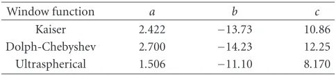
Table3: Estimate coefficients for parameterAcor.
Window function a b c
Kaiser 2.422 −13.73 10.86 Dolph-Chebyshev 2.700 −14.23 12.25 Ultraspherical 1.506 −11.10 8.170
Since differentiators amplify high-frequency errors such as instrumentation measurement errors, bandlimited diff er-entiators are quite useful. Practical bandlimited differentiator design can be accomplished in terms of a nonrecursive filter whose frequency response is required to satisfy the equations
jω−δp
≤HejωT≤jω+δp
for|ω| ∈0,ωp
,
−jδa
≤HejωT≤jδa
for|ω| ∈
ωa,ωs 2
.
(44) For a bandlimited differentiator, the ideal frequency response is taken as
Hid
ejωT=
jω for|ω| ≤ωc, 0 forωc<|ω| ≤ ωs
2
(45)
with ωc = (ωp+ωa)/2. Straightforward analysis gives the infinite-duration impulse response as
hid(nT)=
ωccos
nωc
nπ −
sinnωc
n2π forn=0,
0 forn=0.
(46)
The transition bandwidth in (33) is
Bt=ωa−ωp. (47)
In DDs, the passband ripple and stopband attenuation are dependant on the cutofffrequency of the differentiator. To account for this, a correction forAaof the form
Aa=Aa−Acor (48)
is required where Aa is the corrected design attenuation whose value replacesAainAlgorithm 1,Aais the desired de-sign attenuation, andAcoris a correction term given by
Acor=aω2c+bωc+c. (49) The values of the coefficients a, b, and c for the Kaiser, Dolph-Chebyshev, and ultraspherical windows are given in
Table 3. Examples of differentiators designed using the win-dow method and Remez algorithm can be found in [10].
5.2. Hilbert transformers
In some digital signal processing applications, it is neces-sary to form a special version of the input signalx(nT), des-ignated ˜x(nT), with a frequency spectrum equal to that of x(nT) for the positive Nyquist interval and zero for the neg-ative Nyquist interval [10]. Signals of this type are referred to asanalytic signalsand can be generated by a complex filter
with frequency response
HA
ejωT=1 +jHejωT, (50)
whereH(ejωT) is a Hilbert transformer which has an ideal frequency response given by
HejωT=
−j for 0< ω < ωs 2, j for −ωs
2 < ω <0.
(51)
Filters that perform this operation find application in frequency-division multiplexing systems using single-sideband modulation. Hilbert transformers can be designed in terms of a nonrecursive filter whose frequency response is required to satisfy the equations
j1−δp
≤HejωT≤ j1+δ
p
forω∈
ωp1,ωs
2
,
j−1−δp
≤HejωT≤ j−1+δp
forω∈
−ωs
2,−ωp1
.
(52)
Straightforward analysis gives the infinite-duration impulse response as
hid(nT)=
2 nπsin
2nπ
2 forn=0,
0 forn=0.
(53)
The transition bandwidth in (33) is
Bt=2ωp1. (54)
Like differentiators, it was found that Hilbert transformers require a correction forAaof the form
Aa=Aa+Acor, (55)
whereAais the corrected design attenuation whose value re-placesAa inAlgorithm 1,Aa is the desired design attenua-tion in dB, and Acor is a correction term given by Acor =
6.414, 5.236, and 6.457 for the Kaiser, Dolph-Chebyshev, and ultraspherical windows, respectively.
6. EXAMPLES
Example1. Design a lowpass filter withωp=1,ωa=1.2 rad/s, andAa=80 dB using the Kaiser, Dolph-Chebyshev, and ul-traspherical windows.
The adjustable parameters for the Kaiser, Dolph-Chebyshev, and ultraspherical windows were calculated as α = 7.857, β = 2.803, and β = 2.574, respectively. The additional parameter calculated for the ultraspherical win-dow was µ = 0.6173. The stopband attenuations achieved were 79.38, 82.27, and 79.36 dB with transition bandwidths 0.1987, 0.1994, and 0.1965 rad/s, respectively.
the estimated value ofβ. Thenβis reestimated using an ad-justed design attenuationAa=Aa−(Aar−Aa) whereAais the desired design stopband attenuation. With this modification, the recalculated parameters assume the values α = 7.926, β = 2.725, and β = 2.596, respectively. The stopband at-tenuations were 80.03, 79.96, and 79.83 dB with transition bandwidths 0.2005, 0.1923, and 0.1983 rad/s, respectively. The filter lengths required to achieve the specifications were N = 159 for the Kaiser window, N = 165 for the Dolph-Chebyshev window, andN=153 for the ultraspherical win-dow.Figure 7shows the amplitude responses of the designed filters.
Example2. Design a bandstop filter withωp1 = 0.5,ωa1 =
0.7,ωa2 = 2.0,ωp2 = 2.2 rad/s, andAa = 40 dB using the Kaiser, Dolph-Chebyshev, and ultraspherical windows.
The adjustable parameters for the Kaiser, Dolph-Chebyshev, and ultraspherical windows were calculated as α = 3.395, β = 1.471, and β = 1.391, respectively. The additional parameter calculated for the ultraspherical win-dow was µ = 0.5960. The stopband attenuations achieved were 41.34, 37.36, and 38.40 dB with transition bandwidths 0.1963, 0.2027, and 0.2033 rad/s, respectively. Using the modification discussed in Example 1 to improve stopband attenuation accuracy, the recalculated parameters assume the valuesα=3.235,β=1.554, andβ=1.420, respectively. The stopband attenuations were 39.92, 40.07, and 39.94 dB with transition bandwidths 0.1905, 0.2188, and 0.2125 rad/s, re-spectively. The filter lengths required to achieve the specifi-cations wereN =73 for the Kaiser window,N=73 for the Dolph-Chebyshev window, andN = 67 for the ultraspher-ical window.Figure 8shows the amplitude responses of the designed filters.
Example 3. Design a Hilbert transformer with ωp1 =
0.2 rad/s andAp=80 dB using the Kaiser, Dolph-Chebyshev, and ultraspherical windows.
The adjusted design attenuations from (55) for the Kaiser, Dolph-Chebyshev, and ultraspherical windows were calculated asAa =86.41, 85.24, and 86.46, respectively. The adjustable parameters were calculated as α = 8.564, β = 2.983, andβ =2.789, respectively, while the additional pa-rameter for the ultraspherical window was calculated asµ= 0.6445. The design attenuations achieved were 80.12, 79.59, and 79.39 dB with transition bandwidths 0.3941, 0.3889, and 0.3847 rad/s, respectively. Using the modification dis-cussed in Example 1 to improve design attenuation accu-racy, the recalculated parameters assume the values α = 8.550,β = 2.997, andβ = 2.809, respectively. The attenu-ations were 79.96, 80.01, and 79.93 dB with transition band-widths 0.3935, 0.3912, and 0.3879 rad/s, respectively. The fil-ter lengths required to achieve the specifications wereN=88 for the Kaiser window, N = 90 for the Dolph-Chebyshev window, andN=86 for the ultraspherical window.Figure 9
shows the amplitude responses of the designed Hilbert trans-formers.
Linear passband gain
0 0.5 1
0.9999 1 1.0001
0 0.5 1 1.5 2 2.5 3
Frequency (rad/s)
−120
−100
−80
−60
−40
−20 0
Gain
(dB)
(a)
Linear passband gain
0 0.5 1
0.9999 1 1.0001
0 0.5 1 1.5 2 2.5 3
Frequency (rad/s)
−120
−100
−80
−60
−40
−20 0
Gain
(dB)
(b)
Linear passband gain
0 0.5 1
0.9999 1 1.0001
0 0.5 1 1.5 2 2.5 3
Frequency (rad/s)
−120
−100
−80
−60
−40
−20 0
Gain
(dB)
(c)
0 0.5 1 1.5 2 2.5 3 Frequency (rad/s)
−70
−60
−50
−40
−30
−20
−10 0 10
Gain
(dB)
(a)
0 0.5 1 1.5 2 2.5 3
Frequency (rad/s)
−70
−60
−50
−40
−30
−20
−10 0 10
Gain
(dB)
(b)
0 0.5 1 1.5 2 2.5 3
Frequency (rad/s)
−70
−60
−50
−40
−30
−20
−10 0 10
Gain
(dB)
(c)
Figure 8: Example 2: amplitude responses of bandstop filters designed using various window functions. (a) Kaiser window. (b) Dolph-Chebyshev window. (c) Ultraspherical window.
Linear passband gain
1 2 3
0.9999 1 1.0001
0 0.5 1 1.5 2 2.5 3
Frequency (rad/s) 0
0.2 0.4 0.6 0.8 1
Linear
gain
(a)
Linear passband gain
1 2 3
0.9999 1 1.0001
0 0.5 1 1.5 2 2.5 3
Frequency (rad/s) 0
0.2 0.4 0.6 0.8 1
Linear
gain
(b)
Linear passband gain
1 2 3
0.9999 1 1.0001
0 0.5 1 1.5 2 2.5 3
Frequency (rad/s) 0
0.2 0.4 0.6 0.8 1
Linear
gain
(c)
7. CONCLUSIONS
An efficient method for designing nonrecursive digital fil-ters based on the ultraspherical window has been proposed. Economies in computation are achieved in two ways. First, through an efficient formulation of the window coefficients, the amount of computation required is reduced to a small fraction of that required by the standard methods. Second, the filter length and the independent window parameters that would be required to achieve prescribed specifications in lowpass, highpass, bandpass, and bandstop filters as well as in digital differentiators and Hilbert transformers are efficiently determined through empirical formulas. Experimental re-sults indicate that the ultraspherical window yields lower or-der filters relative to designs obtained using a variety of other known windows including the Kaiser, Dolph-Chebyshev, and Saram¨aki windows. Alternatively, for a fixed filter length the ultraspherical window can provide reduced passband ripple and increased stopband attenuation relative to these win-dows. The weighted-Chebyshev method yields designs that areL∞optimal but these designs require a large amount of
computation, which makes them impractical for applications where the design has to be carried out online in real or quasi-real time.
REFERENCES
[1] T. Saram¨aki, “Finite impulse response filter design,” in Hand-book for Digital Signal Processing, S. K. Mitra and J. F. Kaiser, Eds., Wiley & Sons, New York, NY, USA, 1993.
[2] J. F. Kaiser, “Nonrecursive digital filter design using theI0-sinh
window function,” inProc. IEEE Int. Symp. Circuits and Sys-tems (ISCAS ’74), pp. 20–23, San Francisco, Calif, USA, April 1974.
[3] T. Saram¨aki, “A class of window functions with nearly mini-mum sidelobe energy for designing FIR filters,” inProc. IEEE Int. Symp. Circuits and Systems (ISCAS ’89), vol. 1, pp. 359– 362, Portland, Ore, USA, May 1989.
[4] C. L. Dolph, “A current distribution for broadside arrays which optimizes the relationship between beamwidth and side-lobe level,”Proc. IRE, vol. 34, pp. 335–348, 1946. [5] R. Streit, “A two-parameter family of weights for
nonrecur-sive digital filters and antennas,”IEEE Trans. Acoust., Speech, Signal Processing, vol. 32, no. 1, pp. 108–118, 1984.
[6] A. G. Deczky, “Unispherical windows,” in Proc. IEEE Int. Symp. Circuits and Systems (ISCAS ’01), vol. 2, pp. 85–88, Syd-ney, NSW, Australia, May 2001.
[7] S. W. A. Bergen and A. Antoniou , “Generation of ultraspher-ical window functions,” inProc. 11th European Signal Process-ing Conference (EUSIPCO ’02), vol. 2, pp. 607–610, Toulouse, France, September 2002.
[8] S. W. A. Bergen and A. Antoniou, “Design of ultraspheri-cal window functions with prescribed spectral characteris-tics,”EURASIP Journal on Applied Signal Processing, vol. 2004, no. 13, pp. 2053–2065, 2004.
[9] D. Johnson and J. Johnson, “Low-pass filters using ultraspher-ical polynomials,”IEEE Trans. Circuits and Systems, vol. 13, no. 4, pp. 364–369, 1966.
[10] A. Antoniou,Digital Signal Processing: Signals, Systems, and Filters, McGraw-Hill, New York, NY, USA, 2005.
[11] T. Parks and J. McClellan, “Chebyshev approximation for nonrecursive digital filters with linear phase,”IEEE Trans. Cir-cuits and Systems, vol. 19, no. 2, pp. 189–194, 1972.
[12] J. McClellan and T. Parks, “A united approach to the design of optimum FIR linear-phase digital filters,”IEEE Trans. Circuits and Systems, vol. 20, no. 6, pp. 697–701, 1973.
[13] D. J. Shpak and A. Antoniou, “A generalized Remez method for the design of FIR digital filters,”IEEE Trans. Circuits and Systems, vol. 37, no. 2, pp. 161–174, 1990.
[14] S. H. Nawab, A. V. Oppenheim, A. P. Chandrakasan, J. M. Winograd, and J. T. Ludwig, “Approximate signal process-ing,”Journal of VLSI Signal Processing Systems, vol. 15, no. 1-2, pp. 177–200, 1997.
[15] J. T. Ludwig, S. H. Nawab, and A. P. Chandrakasan, “Low-power digital filtering using approximate processing,”IEEE J. Solid-State Circuits, vol. 31, no. 3, pp. 395–400, 1996. [16] C. J. Pan, “A stereo audio chip using approximate processing
for decimation and interpolation filters,”IEEE J. Solid-State Circuits, vol. 35, no. 1, pp. 45–55, 2000.
[17] M. Abramowitz and I. A. Stegun, Eds.,Handbook of Math-ematical Functions, vol. 55 ofNational Bureau of Standards Applied Mathematics Series, US Government Printing Office, Washington, DC, USA, 1964.
[18] L. R. Rabiner, J. F. Kaiser, O. Herrmann, and M. T. Dolan, “Some comparisons between FIR and IIR digital filters,” Bell System Technical Journal, vol. 53, no. 2, pp. 305–331, 1974.
[19] O. Herrmann, L. R. Rabiner, and D. S. K. Chan, “Practical design rules for optimum finite impulse response low-pass digital filters,”Bell System Technical Journal, vol. 52, no. 6, pp. 769–799, 1973.
[20] J. W. Adams, “FIR digital filters with least-squares stopbands subject to peak-gain constraints,”IEEE Trans. Circuits and Sys-tems, vol. 38, no. 4, pp. 376–388, 1991.
[21] W. Cheney and D. Kincaid,Numerical Mathematics and Com-puting, Brooks/Cole, Pacific Grove, Calif, USA, 1995. [22] F. J. Harris, “On the use of windows for harmonic analysis
with the discrete Fourier transform,”Proc. IEEE, vol. 66, no. 1, pp. 51–83, 1978.
[23] A. H. Nuttall, “Some windows with very good sidelobe be-havior,”IEEE Trans. Acoust., Speech, Signal Processing, vol. 29, no. 1, pp. 84–91, 1981.
[24] S. K. Mitra,Digital Signal Processing: A Computer-Based Ap-proach, McGraw-Hill, New York, NY, USA, 1998.
[25] M. I. Skolnik, Ed.,Radar Handbook, McGraw-Hill, New York, NY, USA, 1990.
[26] K. Ogata, Ed.,Modern Control Engineering, Prentice-Hall, Up-per Saddle River, NJ, USA, 4th edition, 2002.
Stuart W. A. Bergenwas born in Guildford, England, UK, on November 5, 1976. He re-ceived the B.S. degree in electrical engineer-ing from the University of Calgary, Calgary, Alberta, Canada, in 1999. Currently, he is pursuing the Ph.D. degree in electrical en-gineering at the University of Victoria, Vic-toria, British Columbia, Canada. From 1997 to 1998, he was a firmware/hardware de-signer at Wireless Matrix, Calgary, Alberta,
Andreas Antoniou received the B.S. (En-gineering Honors) and Ph.D. degrees in electrical engineering from the University of London in 1963 and 1966, respectively, and is a Fellow of the IEE and IEEE. He served as the Founding Chair of the Depart-ment of Electrical and Computer Engineer-ing, University of Victoria, Victoria, British Columbia, Canada, from July 1, 1983, to June 30, 1990, and is now Professor