Time-Frequency Analysis Using Warped-Based
High-Order Phase Modeling
Cornel Ioana
ENSIETA, E3I2 Research Centre, 2 rue Franc¸ois Verny, 29806 Brest, France Email:[email protected]
Andr ´e Quinquis
ENSIETA, E3I2 Research Centre, 2 rue Franc¸ois Verny, 29806 Brest, France Email:[email protected]
Received 7 June 2004; Revised 27 June 2005; Recommended for Publication by Douglas Williams
The high-order ambiguity function (HAF) was introduced for the estimation of polynomial-phase signals (PPS) embedded in noise. Since the HAF is a nonlinear operator, it suffers from noise-masking effects and from the appearance of undesired cross-terms when multicomponents PPS are analyzed. In order to improve the performances of the HAF, the multi-lag HAF concept was proposed. Based on this approach, several advanced methods (e.g., product high-order ambiguity function (PHAF)) have been recently proposed. Nevertheless, performances of these new methods are affected by the error propagation effect which drastically limits the order of the polynomial approximation. This phenomenon acts especially when a high-order polynomial modeling is needed: representation of the digital modulation signals or the acoustic transient signals. This effect is caused by the technique used for polynomial order reduction, common for existing approaches: signal multiplication with the complex conjugated exponentials formed with the estimated coefficients. In this paper, we introduce an alternative method to reduce the polynomial order, based on the successive unitary signal transformation, according to each polynomial order. We will prove that this method reduces considerably the effect of error propagation. Namely, with this order reduction method, the estimation error at a given order will depend only on the performances of the estimation method.
Keywords and phrases:high-order ambiguity function, polynomial phase signal, warping operator.
1. INTRODUCTION
It is well known that there is no distribution of the Cohen’s class which might produce the complete concentration along the instantaneous frequency law (IFL) when this one is a nonlinear function of time. Matching these types of signals
requires a new joint distribution with different instantaneous
frequency and group delay localization properties. One of the
most known techniques [5] is the unitary similarity
transfor-mation. Using this concept it is possible to construct, via the warping operators, distributions to match almost any one-to-one group delay or instantaneous frequency characteris-tics. More precisely, by warping the analyzed signal accord-ing to the nature of its IFL, it is possible to “linearize” the time-frequency content of the considered signal. Neverthe-less, this concept requires the knowledge of the nonlinearity type, necessary to design the warping operators.
An alternative way to better match the nonlinear time-frequency behavior of the analytical signals (i.e., whose phase can be expressed as a finite series expansion) is to use the high-order time-frequency distributions. Since the
polynomial phase signal constitutes a good model in a vari-ety of applications (e.g., radar imagery, mobile
communica-tion systems [2], etc.), the high-order time-frequency
meth-ods have been developed.
Nowadays, these two research fields—generalization of the classical time-frequency distribution and the data model-ing via the polynomial phase signal concept—have received
considerable attention in the literature [1,2,3,4] and the
references therein. It is primarily due to the number of pos-sible applications, especially for signals having a nonlinear time-frequency behavior: underwater signal processing, dig-ital modulations, radar signals, and so forth. Mathematically, a noiseless polynomial phase signal can be modeled as
s(t)=Aexpjφ(t)=Aexp
j
N
k=0 aktk
, (1)
where N is the polynomial order of the phase φ(t),
{ak}k=1,...,N are the polynomial coefficients, andAis the
One of the first approaches to estimate the parameters of
the PPSs is high-order ambiguity function (HAF) [1] which
provides good results for high signal-to-noise ratio. The un-derlying idea is the transformation of the signal in a nonlin-ear way in order to obtain a tone whose frequency is directly
related to the corresponding polynomial coefficient. The
es-timation accuracy of this method has been devised in [6].
Nevertheless, since the HAF is a nonlinear method, it suffers
from three basic problems: (1) noise-masking effects for low
signal-to-noise ratios (SNR), (2) cross-terms in the presence of multicomponent PPSs (mc-PPSs), and (3) propagation of the approximation error from an order to other.
Recently, different methods have been proposed in
or-der to eliminate the first two limitations. The key point is to use the multilag concept in the HAF computing
proce-dure [2]: using a set of distinct lags, it is possible to
elim-inate the cross-terms and to improve the noise robustness. Moreover, multiplying the HAFs obtained for some lag sets (Product HAF—PHAF), the performances related to noise
robustness and cross-terms effect are considerably improved
with respect to multilag HAF (mlHAF) [2].
Since the Wigner-Ville distribution constitutes the clas-sical tool for chirp signal processing, a natural way to esti-mate the nonlinear IFL of a PPS is based on the polynomial
Wigner-Ville distribution (PWVD) introduced in [3]. The
concept of this method is based on the creation, in the time-frequency domain, of a delta function around the IFL of the signal. Later, the L-Wigner distribution is introduced in or-der to provide a good concentration around the IFL, preserv-ing the interestpreserv-ing properties of the Wigner-Ville
distribu-tion. These two concepts have been generalized in [7]
start-ing with the definition of the high-order polynomial deriva-tives decompositions in terms of a linear combination of the translated version of the polynomial. The generalized ambi-guity function and the generalized Wigner distribution were also proposed.
An alternative way for the estimation of the PPS param-eters is the use of the Bayesian-like procedure. An interesting approach, based on Markov chain Monte Carlo methods for estimation of the a posteriori densities of the polynomial
pa-rameters, is proposed in [8]. The aim of this work deals with
a direct estimation of the polynomial coefficients, contrary
to the works previously mentioned.
In practical application, the use of the polynomial mod-eling procedures requires to set up some parameters. Namely, for the high-order ambiguity function computation, a lag set has to be defined. This problem has been the subject of
sev-eral works. In [5], the authors proposed a criterion based
on the minimization of estimation variances. This work has
been generalized in [2] in the case of PHAF. Alternatively, by
using two coprime lag values, we can improve both the es-timation accuracy and the evaluation of signal component
number [9].
In spite of the improved performances of these
ap-proaches, effect of propagation error remains a serious
draw-back when trying to estimate a high nonlinear IFL (underwa-ter transitory signals, digital modulations, etc.). More
specif-ically, this effect reduces drastically the approximation order
for which an accurate estimation of the IFL is furnished. This
effect, firstly analyzed in [5], is caused by the polynomial
or-der compensation, currently performed by multiplying the
signal with the reference exp{−jaktk}, whereakis the
esti-mation ofkth-order coefficient.
Thence, one way to reduce the error propagation effect
is to use a new method for polynomial order reduction. The method proposed in this paper is based on the polynomial order reduction by warping successively the analyzed signal.
Conventionally, a warping operator is designed to “lin-earize” the time-frequency behavior of the analyzed signal. For time-frequency analysis purposes, this “linearization” is taken into account by applying a classical time-frequency distribution (e.g., Wigner-Ville Distribution—WVD) on the warped signal. In this paper, we propose an alternative use of the warping operator concept.
We design a warping operator whose effect will be the
polynomial order reduction. In the context of the
polyno-mial phase modeling, this effect will be taken into account by
computing the mlHAF of the warped signal. Furthermore, through several examples and performance analysis, we will
prove that this method reduces considerably the effect of
er-ror propagation.
This paper is organized as follows. InSection 2, the
con-cept of the mlHAF is presented.Section 3describes the
ma-jor limitation of the mlHAF, related to the error propagation
effect. The main tools introduced in this paper—“unitary
operators”—will be shortly explained inSection 4.
Further-more, a new method for order compensation will be
de-picted in Section 5. Several signal processing examples will
be presented inSection 6.Section 7presents some remarks
and ideas for future works.
2. MULTILAG HIGH-ORDER AMBIGUITY FUNCTION
The high-order ambiguity function (HAF) was originally de-signed for estimation of a single component, constant
ampli-tude PPS, given by the relation (1). The HAF is defined as the
Fourier transform of the high-order instantaneous moments
(HIM) given, for a signals(t), by the following relation:
HIMK
s(t);τ
K−1
q=0
s(∗q)
(t−qτ)
K−1
q
, (2)
whereKis the HIM order,τis the lag, and (∗q) is an operator
defined as
s(∗q)(t)= s
(t), ifqis even,
s∗(t), ifqis odd, (3)
where q is the number of conjugate operator “∗”
applica-tions. From the computational point of view, the main
prop-erty of the HIM [1] states that theKth-order HIM can be
computed as the 2nd-order HIM of the (K−1)th-order HIM:
HIMK
s(t);τ=HIM2
HIMK−1
Another remarkable property, which makes HIM an at-tractive tool in the polynomial phase modeling context, is
that theNth-order HIM of a PPS given in (1) is reduced to
a constant amplitude harmonic with amplitude A2N−2
,
fre-quency ˜ωN, and phase ˜φN [1]:
HIMN
s(t);τ=A2N−1
expjω˜N·t+ ˜φN
, (5)
where
˜
ωN =N!τN−1aN,
˜
φN =(N−1)!τN−1aN−1−0.5N!(N−1)τNaN.
(6)
A natural idea to take advantage of this property is to
compute the Fourier transform of Nth-order HIM, which
leads to the HAF definition [1]:
HAFN[s;ω,τ]=
∞
−∞HIMN
s(t);τe−jωtdt. (7)
Obviously, taking into consideration the relation (5), the
Nth-order HAF of the signal given in (1) peaks at the
fre-quency ˜ωN. This property gives a practical method for
poly-nomial coefficients estimation [1]. Starting with the
highest-order coefficientaN, the maximum of the HAF is evaluated
at each order. TheNth-order polynomial coefficient is
esti-mated via
aN = 1
N!τN−1arg max
ω
HAFN(s;ω,τ). (8)
Using this estimation, the effect of the phase term of the
higher order is removed:
s(N−1)(t)=s(t)·e−jaNtN. (9)
Once theNth-order is reduced, the (N−1)th-order HAF
is computed. The coefficientaN−1is also estimated thanks to
relation (8). The algorithm is iterated through the inferior
orders until all polynomial coefficients are estimated.
As it was illustrated in [1,2], the classical procedure for
polynomial phase modeling, based on HAF method, is
prac-tically affected by some limitations regarding the noise
ro-bustness and the cross-terms presence. To overcome these problems, the multilag HAF (mlHAF) concept has been
ini-tially proposed in [2]. In fact, the mlHAF is based on the
gen-eralization of the high-order instantaneous moment HIM
[2], based on the property expressed in relation (4):
mlHIMN
s(t);τN−1
=mlHIMN−1
st+τN−1
;τN−2
×mlHIM∗N−1st−τN−1
;τN−2
,
(10)
where τN = (τ1,τ2,. . .,τN) is the set of lags. Applying the
Fourier transform, exactly as for the case of the HAF (7), we
obtain the mlHAF of the signals(t):
mlHAFN
s;ω,τN
= ∞
−∞mlHIMN
s(t);τN
e−jωtdt. (11)
In practical applications, the choice of the lags set (τ1,τ2,. . .,τN) is often difficult to do. One possible solution,
proposed in [2], isNi=−11τi=const=τN−1. Based on the
res-olution capability criterion [2], it can be shown thatτ=L/N
(L-signal length) represents the optimal choice.
Using the mlHAF computed for a lag set provided in this
manner, the polynomial coefficients are estimated with
rela-tion (8). In [2], the performances of the mlHAF-based
proce-dure are proved. Nevertheless, there are still some limitations related to the noise reduction and cross-terms. To surmount
these limitations, Barbarossa et al. [2] introduced the
prod-uct HAF (PHAF). The mlHAFs computed, via relation (11),
for different lag sets:
T=τ(l) N−1
1≤l≤P; τ (l) N−1=
τi
1≤i≤N−1, (12)
are multiplied, obtaining in this way a robust method and a cross-term free representation:
PHAF(f;T)=
P
l=1
mlHAFN
s; N−1
i=1 τ (l)
i N−1
i=1 τ (1)
i
f,τ(Nl)−1
, (13)
wherePis the number of the lags set used at each order.
The next example illustrates the PHAF superiority
(Figure 1b) with respect to mlHAF-based procedure. We
consider, as a test signal, a two component 3rd-order PPS:
s(t)=exp
j2π
0.25·t−0.05
L t 2+0.28
L2 t 3
+ exp
j2π
0.45·t+0.15
L t 2−0.12
L2 t 3
(L=306)
(14)
embedded in an additive white Gaussian noise (SNR =
10 dB).
In order to illustrate the differences between mlHAF and
PHAF, Figure 1 is structured in two parts associated with
both methods: Figure 1a—mlHAF and Figure 1b—PHAF.
Each part contains six subplots organized as follows: each subplot row is associated to a signal component and, inside the row, each subplot corresponds to mlHAF estimation of
order 3 (right subplot) to 1 (left subplot). Thex-axis of each
subplot corresponds to the frequency and they-axis to
mag-nitude. Values of estimated coefficients are also given. The
same rule is used throughout this paper.
As illustrated in this figure, in the mlHAF case, the
reduced number of lags affects the IFL estimation
qual-ity (Figure 1a). This result can be explained by the
spu-rious spectral peaks which appear in the mlHAF spectra
(Figure 1a—the subplots associated to each component at a
given order). Consequently, the estimation of the polynomial
coefficients becomes poor especially for lower orders.
On the other hand, the PHAF solves the noise robust-ness and multicomponent estimation problems, providing
also a correct IFL estimation (Figure 1b). The PHAF-based
estimated values of the polynomial coefficients are close to
the real ones. This is also illustrated inFigure 1b by a
0 0.2 0.4 0.6 0.8 1
Comp. no. 1: 1st-order mlHAF
N
o
rm
aliz
ed
mag
nitude
−0.5 0 0.5
f
Est. a1=0.2557
0 0.2 0.4 0.6 0.8 1
Comp. no.1: 2nd order mlHAF
N
o
rm
aliz
ed
mag
nitude
−0.5 0 0.5
f
Est. a2=0.0002953
0 0.2 0.4 0.6 0.8 1
Comp. no. 1: 3rd-order mlHAF
N
o
rm
aliz
ed
mag
nitude
−0.5 0 0.5
f
Est. a3=3.637e-006
0 0.2 0.4 0.6 0.8 1
Comp. no.2: 1st order mlHAF
N
o
rm
aliz
ed
mag
nitude
−0.5 0 0.5
f
Est. a1=0.4104
0 0.2 0.4 0.6 0.8 1
Comp. no. 2: 2nd-order mlHAF
N
o
rm
aliz
ed
mag
nitude
−0.5 0 0.5
f
Est. a2=0.002424
0 0.2 0.4 0.6 0.8 1
Comp. no. 2: 3rd-order mlHAF
N
o
rm
aliz
ed
mag
nitude
−0.5 0 0.5
f
Est. a3=1.576e-005
0 0.1 0.2 0.3 0.4 0.5
Fre
q
u
en
cy
(nor
maliz
ed)
−150−100−50 0 50 100 150 Theoretical Estimated Time (samples)
(a)
Figure1: (a) mlHAF-based procedure versus (b) PHAF-based procedure.
the associated polynomial coefficient. Namely, as illustrated
by the subplots associated to each polynomial order, the
co-efficients belonging to each signal component are accurately
estimated.
Still, this “nice” result was obtained for a signal having a smooth time-frequency behavior. If this condition is not ver-ified (the signals whose phases are modeled by a high
poly-nomial order, such as underwater transient signals [17]), a
limitation that cannot be neglected acts. It is related to the
error propagation effect evaluated in the next section.
3. ERROR PROPAGATION EFFECT IN POLYNOMIAL PHASE MODELING
The approach presented in this paper constitutes a
partic-ularization of the results obtained in [5]. In this section,
we will evaluate the dependence expression of the errors for two consecutive orders and for a particular value of the lag. The purpose is to provide a suggestive overview on the error
propagation effect.
We consider the signal given in (1) and we denote with
aN the estimation of theNth-order polynomial coefficient.
In real applications [1], since the mlHAF-based polynomial
coefficients evaluation involves a spectral estimation step (8)
of a discrete sequence, the estimated value differs from the
theoretic one by εN = aN −aN. This quantity denotes the
approximation error and it is directly related to the number
of Fourier points and the SNR [2]. Using this estimate, we
remove theNth-order coefficient via (9). Consequently, the
corresponding (N−1)th-order PPS becomes
s(N−1)(t)=Aej(Nk=−01aktk+(aN−aN)tN)=Aej
N−1
k=0aktk·ejεNtN.
(15)
For simplicity reasons we considerA=1. With relation
(2) and the notation ˜s(t)=ejkN=−01aktk, the (N−1)th-order
HIM is expressed as
HIMN−1
s(N−1)(t);τ
= N−1
q=0
˜
s(∗q)(t−qτ)
N−1
q
N−1
q=0
ejεN(−1)q(t−qτ)N N−1
q
.
(16)
According to the property stated by the relation (5), we
can write
HIMN−1
s(N−1)(t);τ=ej[(N−1)!τN−2aN−1t+φN−1], (17)
where φN−1 = (N − 2)!τN−2aN−2 − 0.5(N − 1)!(N
−2)τN−1a
0 0.2 0.4 0.6 0.8 1
Comp. no. 1: 1st-order PHAF
N o rm aliz ed mag nitude
−0.5 0 0.5
f
Est. a1=0.2482
0 0.2 0.4 0.6 0.8 1
Comp. no.1: 2nd order PHAF
N o rm aliz ed mag nitude
−0.5 0 0.5
f
Est. a2=0.0001629
0 0.2 0.4 0.6 0.8 1
Comp. no. 1: 3rd-order PHAF
N o rm aliz ed mag nitude
−0.5 0 0.5
f
Est. a3=3.117e-006
0 0.2 0.4 0.6 0.8 1
Comp. no. 2: 1st-order PHAF
N o rm aliz ed mag nitude
−0.5 0 0.5
f
Est. a1=0.4497
0 0.2 0.4 0.6 0.8 1
Comp. no. 1: 2nd-order PHAF
N o rm aliz ed mag nitude
−0.5 0 0.5
f
Est. a2=0.0004899
0 0.2 0.4 0.6 0.8 1
Comp. no. 2: 3rd-order PHAF
N o rm aliz ed mag nitude
−0.5 0 0.5
f
Est. a3=1.2676e-006
0 0.1 0.2 0.3 0.4 0.5
Fre q u en cy (nor maliz ed)
−150−100−50 0 50 100 150 Theoretical Estimated Time (samples)
(b)
Figure1: Continued.
This expression is the consequence of the main HAF
property previously presented: the (N−1)th-order HIM of a
given signal is a sinusoid with an angular frequency related,
via (6), to the (N−1)th-order polynomial coefficient.
Nev-ertheless, due to the measurement error which occurs for the
Nth order, the coefficientaN−1is not equal to the theoretical
(N−1)th-order polynomial coefficient,aN−1, of signals. To
find the relation between the errors at two successive orders,
N and (N−1), we evaluate the two products which appear
in relation (16).
With property (5) and observing that ˜s(t)=ejkN=−01aktkis
an (N−1)th-order PPS, which could be ideally obtained if
εN =0, the first product becomes
HIMN−1
˜ s(t);τ=
N−1
q=0
˜
s(∗q)(t−qτ)
N−1
q
=ej[(N−1)!τN−2a
N−1t+φN−1],
(18)
whereφN−1can be expressed, thanks to (6), as follows:
φN−1=(N−2)!τN−2aN−2−0.5(N−1)!(N−2)τN−1aN−1.
(19)
The second term of the product in (16) can be
writ-ten, applying the Newton’s binomial formula to the term
(t−qτ)N, as
N−1
q=0
ejεN(−1)q(t−qτ)N N−1
q
=exp
jεN N−1
q=0
(−1)qN−1
q
(t−qτ)N
=exp
jεN N−1
q=0
(−1)qN−1
q N
i=0
N
i
ti(−q)N−iτN−i
.
(20)
Since the peak corresponding to a polynomial coefficient
is extracted by the HAF (i.e., Fourier transform of the HIM), at a given order, in the expression of the corresponding HIM,
we always look for the term which weightst. Consequently,
from (20), we retain the term
exp
jNεNτN−1 N−1
q=0
(−1)qN−1
q
(−q)N−1
0 200 400 600 800 1000
Er
ro
r
1 2 3 4 5 6 7
Order
Figure2: Error propagation effect (N=8,L=10).
Introducing (17), (18), and (21) in (16) and identifying
the terms weightingt, we obtain the relation between the
es-timation of the (N−1)th-order polynomial coefficient (aN),
the theoretical (N−1)th-order polynomial coefficient (aN),
and the error at orderN(εN):
(N−1)!τN−2a
N−1
=(N−1)!τN−2a
N−1+NεNτN−1 N−1
q=0
(−1)qN−1
q
(−q)N−1.
(22)
With the notationεN−1=aN−1−aN−1, (22) becomes
εN−1= NεNτ
(N−1)!
N−1
q=0
(−1)qN−1
q
(−q)N−1
! "
Sq
. (23)
In [12], it is shown that the summationSq is (N−1)!.
With this result, the dependence between the errors existing for two successive polynomial orders is
εN−1=NεNτ (24)
and, using the optimal value of the lag previously defined,
that is,τ=L/N, we get
εN−1=LεN. (25)
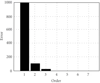
This relation shows that the error existing at a given order
is transmitted at the inferior order by multiplication ofL—
the number of samples of the signal.Figure 2illustrates this
dependence forL=10 samples.
From this figure, it can be observed that even if the
mea-surement error for the highest order is insignificant, its effect
through the lower orders becomes deeply disturbing.
On the other hand, we remark that this effect becomes
“visible” after the polynomial estimation at some orders. It
explains why the error propagation effect does not affect
the polynomial estimation when a small approximation or-der is required (3 or 4). Anyway, there are many situations which impose a high approximation order: digital modula-tions, transitory signals, and so forth. One example is given
in Figure 3 where we process, via the PHAF-based phase
modeling method, a sixth-order PPS whose analytical form is given by
s(t)=expj2π0.17·t−9.7·10−4·t2−2.35·10−7·t3
+ 3.8·10−8·t4+ 2.8·10−10·t5
−3.29·10−13·t6.
(26)
The theoretical IFL is plotted inFigure 3b. Note that the
SNR is about 30 dB.
The PHAF-based estimation procedure was applied, starting with order 6. The successive PHAF spectra are
de-picted inFigure 3a. The values of the estimated coefficients
are depicted in theTable 1. They are obtained via the relation
aN = 1/N!τN−1arg maxf|PHAFN(f;T)|, where τ = L/N
(Lis the signal length) andαN=arg maxf|PHAFN(f;T)|is
the normalized frequency coordinate associated to the most
energeticNth-order PHAF peak. This value ranges between
−0.5 and 0.5 and, for the considered example, they are given
inTable 1. Dividing such value byN!τN−1explains the very
small values of the polynomial coefficients at the high orders.
For higher orders (6, 5), PHAF performs quite well: the
propagation error is insignificant, but its effect is
accumu-lated and it becomes disturbing for lower orders (down to 5). The error propagation is materialized by a more accentuated
presence of spurious peaks with order decreasing (Figure 3a).
The estimated coefficients (Table 1) are different in
compar-ison with the real coefficients given in (26). Consequently,
the estimation of the polynomial coefficient is not correct
(Figure 3b); the evaluated IFL does not match the correct
time-frequency behavior of the analyzed PPS.
This example illustrates the error propagation effect that
was analyzed in this section. We have shown that this effect is
caused by the classical phase removing the step illustrated in
(15).
In the Section 5 we propose an alternative method to
reduce the polynomial order. This method is based on the warping technique concept briefly presented in the next sec-tion.
4. WARPING OPERATOR PRINCIPLE
Unitary similarity transformations furnish a simple powerful tool for generating new classes of joint distributions based
on concepts different from time, frequency, and scale [10].
These new signal representations focus on the critical charac-teristics of large classes of signals, and, hence, prove useful for representing and processing signals that are not well matched by current techniques. Actually, it is possible to construct (via unitary transformations) distributions to match almost any one-to-one group delay or instantaneous frequency
0 0.2 0.4 0.6 0.8 1
N
o
rm
aliz
ed
mag
nitude
−0.5 0 0.5
Normalized frequency 6th-order PHAF
0 0.2 0.4 0.6 0.8 1
N
o
rm
aliz
ed
mag
nitude
−0.5 0 0.5
Normalized frequency 5th-order PHAF
0 0.2 0.4 0.6 0.8 1
N
o
rm
aliz
ed
mag
nitude
−0.5 0 0.5
Normalized frequency 4th-order PHAF
0 0.2 0.4 0.6 0.8 1
N
o
rm
aliz
ed
mag
nitude
−0.5 0 0.5
Normalized frequency 3rd-order PHAF
0 0.2 0.4 0.6 0.8 1
N
o
rm
aliz
ed
mag
nitude
−0.5 0 0.5
Normalized frequency 2nd-order PHAF
(a)
0 0.2 0.4 0.6 0.8 1
N
o
rm
aliz
ed
mag
nitude
−0.5 0 0.5
Normalized frequency 1st-order PHAF
0 0.1 0.2 0.3 0.4 0.5
F
req
uency
(nor
m
aliz
ed)
−200 −100 0 100 200
Theoretical IFL Estimated IFL
Time (samples)
(b)
Figure3: PHAF-based phase modeling of a sixth-order PPS. (a) Classical phase removing. (b) Theoretical and estimated IFL.
Table1: Polynomial coefficients estimated by PHAF.
α1 α2 α3 α4 α5 α6
Values 0.425 −0.112 −0.0961 0.084 0.4714 −0.0817
a1 a2 a3 a4 a5 a6
Values 0.425 −3.634·10−4 −1.54·10−6 7.82·10−9 2.8·10−10 −3.29·10−13
transformation[10], defined for a signals(t) as an operatorU
onL2(R), whose effect is given by
(Us)(x)=w˙(x)1/2sw(x), (27)
wherewis a smooth, one-to-one function, including a large
subclass of unitary transformations [10]. The term ˙w(x)
de-notes the first-order derivative of the functionw. The
func-tions w(x) = ex andw(x) = |x|ksgn(x), k = 0, provide
examples of useful warpings [13,14]. Generally, these
func-tions are chosen to ensure the “linearization” of the signal time-frequency behavior. So, for a signal expressed as
s(t)=ej2π(f0t+βm(t)), (28)
wherem(t) is the frequency modulation law andβthe rate
modulation, the associated warping function is given by [10]
1 2 3 L−1 L x
1 2 3 L−1 L xe
usamples
Interpolation knowingw(x)
1 x
w
Figure4: Warping technique: implementation scheme.
As shown in [10], the application of this operator
pro-duces the linearization of the time-frequency content. Practically, the application of a warping operator is sim-ilar to the coordinate changing stated by the warping law.
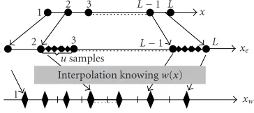
In [17] an efficient implementation scheme is proposed:
the warping operator application effect is done according to
stages depicted inFigure 4.
Firstly, the original axis of the signal, whose length isL,
is oversampled with a rate u. The new finest sampling grid
leads to a more accurate evaluation of the new coordinates
[17]. This operation is done in the second stage. Using the
discrete version of the warping function,w(x), we evaluate
the new coordinates. Since the warping function gives gener-ally a noninteger number, an interpolation procedure will be used to generate the appropriate integer coordinates. Then, the warped signal is generated by resampling the signal for these new coordinates.
Furthermore, the linearization of the time-frequency content is taken into account by computing the Wigner-Ville
distribution (WVD) of the warped signal [17]:
WVDUs(˜t, ˜f)=
(Us)
˜ t+τ
2
(Us)∗
˜ t−τ
2
e−j2πf τ˜ dτ.
(30)
The new time-frequency coordinates are related to the
standard ones via [16]
˜
t=w−1(t), f˜= fw˙w−1(t), (31)
wherew−1is the inverse function ofw(t). We note that this
relation is available in the case of time warping operators. An alternative formula can be devised for the frequency warping
operators [16,17].
The following example illustrates the property of warp-ing operators related to the linearization of the time-frequency behavior. For a signal given by
s(t)=ej2π(0.38t−0.02t1.3), (32)
the associated warping operator can be defined as [15]
U1/k:w(t)=t1/k, k=1.3,
˙ w(t)= 1
kt
(1/k)−1. (33)
According to this operator, the mathematical expression of the warped signal is
U1/ks
(t)=ej2π(0.38t1/1.3−0.02t)
. (34)
The evaluation of the WVD of this signal in original time and frequency coordinates leads to a complicate
time-frequency behavior as indicated inFigure 5.
Obviously, the nonlinear time-frequency content of the
original signal (Figure 5a) is transformed, via WVD
com-puted for conventional time-frequency coordinates, in a new nonlinear time-frequency form.
Therefore, in order to take advantage of the warped form of the oversampled signal, the WVD must be computed, via
(30), in the new time and frequency coordinates associated to
the warping operators. Thanks to (31) for the warping
func-tion devised in (33), the new time-frequency coordinates are
written as
˜
t=w−1(t)=tk,
˜
f = fw˙tk= f1 k
tk1/k−1= f kt
1−k (35)
and, fork=1.3,
˜
t=t1.3, f˜= f
1.3t
−0.3
. (36)
As indicated inFigure 4, in order to obtain a more
ac-curate evaluation of the warped time axis, an oversampling
procedure is applied to the original signal [17]. The
oversam-pled signal,su, represented in a finer time axis coordinates,
tu, is warped via (33). The WVD of the warped version of
the oversampled signal ((U1/ksu)(tu), u = 10) is plotted in
Figure 6b. Comparing this figure withFigure 5b, we remark
that the time-frequency content of (U1/ksu)(tu) is less
nonlin-ear than the one of the (U1/ks)(t) (Figure 5b). This is related
to the advantage of the warping application on the oversam-pled signal.
As we can see inFigure 6a, due to the term 0.38t1/1.3
u of the
warped signal (34), nonlinearity is still visible in the interval
of 0÷100 samples. That is, even if the signal is warped after
oversampling, this term is again visible. This nonlinearity is
eliminated by computing, using (30), the WVD for new time
and frequency coordinates depicted in (36). As illustrated in
Figure 6b, the result is a linear time-frequency structure.
This example illustrates the capability of the warping op-erator concept to linearize the time-frequency content of a
signal. As theoretically shown in [17], two steps are involved.
Firstly, the signal is warped according to its modulation na-ture. Secondly, the WVD of warped signal is evaluated, using the new time and frequency coordinates.
Both theoretical and practical issues, previously pre-sented, suppose some knowledge on the time-frequency
na-ture of the signal (the warping function w(t) has to be
0 0.1 0.2 0.3 0.4
f
0 200 400
t
(a)
0 0.1 0.2 0.3 0.4
f
0 200 400
t
(b)
Figure5: WVD of (a) original signal (WVDs(t,f)) and (b) warped signals in conventional time-frequency coordinates (WVDU1/Ks(t,f)).
0 0.5 1
fu
100 200 300 400 500
tu
(a)
0 0.5 1
#
f
0 200 400
#
t
(b)
Figure6: The effect of the warping operator in new time-frequency plane. (a) WVDU1/Ksu(t,f). (b) WVDU1/Ksu(˜t, ˜f).
information is not available (passive sonar and radar fields, recognition of digital modulations, etc.). In order to deal with these situations, many methods have been developed
[18,19]. The common used technique is the signal
decom-position on an extended dictionary composed of elemen-tary functions with nonlinear time-frequency behavior. Af-ter the signal decomposition with such dictionary, the ex-tracted elementary functions are optimally represented in a time-frequency plane, using the associated warping opera-tors. These methods, which constitute the generalization of
the chirplet-transform-based methods [20], are often
lim-ited in practical applications by a required huge dictionary size.
An alternative to characterize the nonlinear time-frequency behavior of an unknown signal is described in the next section. This method is based on the polynomial phase modeling associated with a new polynomial phase removing procedure. The objective is to reduce the error propagation
effect described inSection 3. Conceptually, a warping
oper-ator is designed to replace the polynomial order reduction
stage described in relation (9). This warping operator is
gen-erally defined as
Uk:wk(t)=
t
ak 1/k
, (37)
whereak is the estimation of thekth-order polynomial
co-efficient. The following example illustrates the effect of this
warping operator for a 3rd-order PPS given by
s(t)=ej2π(0.37t−4.6·10−4·t2+3·10−6·t3)
(38)
whose WVD is plotted inFigure 7a.
Applying the warping operator (37) (fork = 3 anda3
close to the real valuea3) to the oversampled version of the
signal (38), we obtain the warped signal
U3su
tu
≈ej2π[0.37(tu/a3)1/3−4.6·10−4(tu/a3)2/3+tu]
=ej2π[0.37(tu/a3)1/3−4.6·10−4(tu/a3)2/3]·ej2πtu, (39)
wheretuis the time axis issued after oversampling (u=10).
As shown in [17] and practically illustrated in the
ex-ample previously presented, the effect of the time-frequency
content linearization provided by a general warping opera-tor is “visible” by the evaluation of the WVD for new time-frequency coordinates.
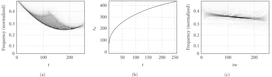
Alternatively, if the warping operator is designed to
re-duce the polynomial order of a signal, its effect will be
de-picted by computing the HIM corresponding to the new polynomial order. Knowing that the 2nd-order HIM is the classical instantaneous correlation function which appears in
the WVD definition [16], the effect of 2nd-order HIM
appli-cation is equivalent to the evaluation of the WVD. For this
reason, we illustrate, in Figure 7c, the WVD of that signal
(39). We remark that a linear time-frequency structure was
0 0.1 0.2 0.3 0.4
F
req
uency
(nor
m
aliz
ed)
0 100 200
t
(a)
0 100 200 300 400
tw
50 100 150 200 250
t
(b)
0 0.1 0.2 0.3 0.4
F
req
uency
(nor
m
aliz
ed)
0 100 200
tw
(c)
Figure7: Polynomial order reduction using the warping operator (37). (a) WVD of original signal. (b) Warping law. (c) WVD of warped signal.
above, that the warping operator defined by (37) has, in
as-sociation with the corresponding HIM, an order-reducing ef-fect.
Applying the warping procedure described inFigure 4,
some artifacts appear in practice (Figure 7c). They are caused
by the errors induced by numerical computations. As illus-trated in these figures, these artifacts are not disturbing since the main linear time-frequency component is much more energetic. However, these errors might be reduced by
increas-ing the oversamplincreas-ing rate u[17]. Nevertheless, from
com-putational tractability point of view, this rate cannot be ar-bitrarily high. In the case of the warping operator defined
by the expression (37), the method for the evaluation of the
value of oversampling parameter uis described in the
ap-pendix.
The polynomial order removing of the warping operator
defined in (27) is used in the following section. Also, we will
prove, in a more rigorous manner, that it is possible to suc-cessively reduce the order of the phase modeling by iterative applications of this warping operator.
5. WARPED-BASED POLYNOMIAL
ORDER REDUCTION
In this section, we will mathematically prove the property of
the warping operator (37) to reduce the polynomial order of
the signal.
We consider anNth-order PPS defined by the relation
(1). Using a modern version of the HAF-based polynomial
modeling procedure (PHAF operator or the approach
pro-posed in [11]), we can obtain an accurate estimate of the
Nth-order polynomial coefficient, denoted byaN. With this
estimation, we design, via (37), the corresponding warping
operator:
wN :t−→UN tw(N)=wN(t)= $
t
aN %1/N
. (40)
Some implementation issues associated to this warping operator are commented in the appendix. Mathematically,
the effect of the associated unitary operatorUon the PPS
is depicted, in the new time coordinate, as
UNs
t(wN)
=A˜exp
jaN $
t
aN
%1/NN
·exp
j
N−1
m=0 am
t(N)
w m
=A˜exp
j
N−1
m=0 am
t(N)
w m
! "
(N−1)th-order PPS(s(N−1))
·exp
jaN aNt
! "
residualr(t)
,
(41)
where
˜ A=A
& ' ' '
( 1
NaN $
t
aN %1/N−1
. (42)
Since all the terms in (42) are known and nonrandom,
the induced amplitude modulation can be compensated, for example, through an amplitude weighting using the inverse
of relation (42).
Therefore, the result of the warping transform of anN
th-order PPS consists in a (K−1)th-order PPS with a new
tem-poral variablet(wN). The (N−1)th-order PHAF of this signal,
with respect to the variablet(wN), peaks to a frequency
loca-tion related, via relaloca-tion (6), to theaN−1coefficient. To prove
that, we compute the (N−1)th-order HIM of theUNssignal:
HIMN−1
UNs(N);τ
=HIMN−1
s(N−1)t(N)
w
;τ·HIMN−1
r(t);τ. (43)
The first term of the product (43) is a sinusoid associated
to the (N−1)th-order polynomial coefficient:
HIMN−1
s(N−1)t(N)
w
;τ=A2N−2
ej(N−1)!aN−1τN−2t(wN) (44)
because it represents the (N−1)th-order HIM of the (N−
From property (4), it is easy to show that the second term
of (41) is 1 forN >2:
HIM2
r(t);τ=ej(aN/aN)t·e−j(aN/aN)(t−τ)=ej(aN/aN)τ,
HIM3
r(t);τ=ej(aN/aN)τ·e−j(aN/aN)τ=1, ..
.
HIMN
r(t);τ=1·1=1, N≥3.
(45)
Consequently, the (N−1)th-order HIM of theUNssignal is
HIMN−1
UNs(N);τ
tw(N)
=A2N−2ej(N−1)!aN−1τN−2t(wN). (46)
As stated by this relation, forN >2, the (N−1)th-order
HIM of the warped signal UNsdoes not contain any term
related to the residualrgiven by (41). Consequently, the
es-timated value of theNth-order coefficient does not act in the
estimation procedure of the (N−1)th order. Actually, from
a theoretical point of view, we could eliminate the|aN|from
the structure of the warping operator defined in (40). In this
case, we should have obtained the same results as in (45): the
Nth-order HIM ofr(t) is 1 forN >2. This proves the
inde-pendence of the estimation procedure at a given order on the
coefficients already estimated.
Hence, as shown in the appendix, the presence of|aN|
in the definition of the warping operator (40) is dictated by
practical reasons: the necessary values of the oversampling rate will have a reasonable value.
Then, we use the PHAF-based method to estimate the
co-efficientaN−1. Via (37), with this new value we construct a
new warping operator used to reduce the (N−1)th order as
described in (41).
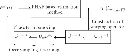
This procedure is iterated until all polynomial coeffi
-cients are estimated. Practically, the new polynomial
estima-tion method is depicted in the block diagram (Figure 8).
Unlike the classical order reduction technique (relation
(9)), the warping-based order reduction eliminates from the
expression of the warped signal the terms related to the es-timation at the higher orders. In consequence, as it is
the-oretically proved by the relations (41) and (46), the
perfor-mances of the PHAF-based estimation procedure
theoreti-cally dependonlyon the result at the given order. This fact,
proved by relations (43), (44), (45), and (46), constitutes the
main important feature of the warping operator (40) and its
use for order reduction (41).
However, as the error analysis (provided through simula-tions) will prove in the next section, the estimation error at a given order is practically independent of the errors which occur for higher orders.
6. SIMULATION RESULTS
To demonstrate the capabilities of the warping-based order reduction, some simulation results will be presented. The method proposed in the previous section will be compared with the conventional PHAF (i.e., the polynomial order
re-duction is done by the classical procedure depicted in (9)).
PHAF-based estimation method
s(m−1) U
ms(m) s(m−1) Ums(m)
s(m)(t) a#
m
m=1,N
Phase term removing
Construction of warping operator
Over sampling + warping
Figure 8: Polynomial coefficient estimation based on warping phase order removing.
Since the PHAF performing for a polynomial order larger
than 3 is influenced by the error propagation effect, we limit
our simulations to the third order. However, as shown in
Section 3, the error propagation effect becomes “visible”
af-ter three iaf-terations. Consequently, the choice of third-order phase modeling in our simulation should be enough to ob-jectively compare the second-order reducing procedures.
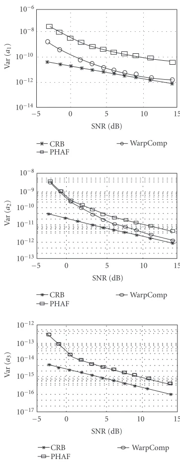
The performances of this new approach are firstly proved in terms of estimation error variances as a function of the SNR. We assumed a 3rd-order PPS, given by the
rela-tion (38), embedded in white Gaussian noise. Two
meth-ods have been compared—PHAF-based estimation method and PHAF-based estimation method with warping-based phase compensation (denoted by “WarpComp” method). Each variance was computed for 500 trials and, for each or-der, it was compared with the Cramer-Rao bound (CRB)
evaluated in [21].
The first plot proves that, for the highest-order, the per-formances of both methods are similar: the estimation of the
highest-order coefficient (a3) depends on the noise level. The
next two pictures show that, using the warping-based phase compensation, the estimation performances remain close to
the CRB as in the case of the highest-order coefficient.
Con-sequently, the performances of this method depend only on
the noise, whereas in the PHAF case they are affected also by
the error propagation phenomenon.
The statistical analysis provided by the Figure 9shows
clearly the reduction of the error propagation effect which
acts in the case of the classical phase order compensation
(re-lation (9)).
The cancellation of the error propagation effect is also
illustrated inFigure 10, using the signal proposed in (14).
The estimated values of the polynomial coefficients and
of the PHAF peaks are depicted inTable 2.
As the figure shows, the proposed method for polynomial order reduction provides a much more accurate estimation of the IFL than methods which use the classical phase order
reduction (for comparison seeFigure 3).
As pictured in the PHAF subplots at each order, the de-pendence between the errors occurred at these orders is prac-tically eliminated: there is a single prominent peak
corre-sponding to the polynomial coefficients. No spurious peaks,
independent of the considered order (Figure 10a), are
identi-fied. Accordingly, these coefficients are accurately estimated
10−14
10−12
10−10
10−8
10−6
Va
r
(
a1
)
−5 0 5 10 15 SNR (dB)
CRB PHAF
WarpComp
10−13
10−12
10−11
10−10
10−9
10−8
Va
r
(
a2
)
−5 0 5 10 15 SNR (dB)
CRB PHAF
WarpComp
10−17
10−16
10−15
10−14
10−13
10−12
Va
r
(
a3
)
−5 0 5 10 15 SNR (dB)
CRB PHAF
WarpComp
Figure9: The estimated variances versus SNR.
order reduction through the procedure based on the warp-ing operators improves considerably the performances of the PHAF-based estimation procedure.
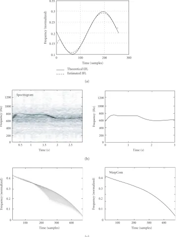
This property is also pointed up inFigure 11, in the case
of some signals of different types: sinusoidal frequency
mod-ulation (SFM) (Figure 11a), a signal emitted by a Diesel
en-gine [23] (Figure 11b), and a signal received from an
under-water mobile emitting a chirp (Figure 11c).
For each of those signal types, we note that the polyno-mial approximations provided by the proposed approach are correctly related to the theoretical IFL or with the informa-tion provided by a classical method (spectrogram). In the
case of the signal emitted by a Diesel engine (Figure 11b), the
polynomial phase approximation provided by the proposed
approach is expressed as
φ(t)=539·t+ 2.32·10−2·t2−1.32·10−6·t3
+ 3.67·10−11·t4−5.4·10−16·t5. (47)
InFigure 11c, we analyze the signal received from an
un-derwater moving source (having a velocity v = 6 m/s and
an accelerationa= 0.07 m/s2; the source moves away from
the receiver). We supposed that the source transmits a chirp
given by exp[j2π(410t+ 2.48t2)] and the receiver sampling
frequency isFs =1000 Hz. In this configuration, as shown
in [24], received signal phase becomes a fourth-order
poly-nomial. Its estimation, provided by the method proposed in this paper, is given by
φ(t)=0.41·t+ 3.82·10−4·t2
−3.15·10−6·t3+ 1.63·10−9·t4. (48)
Its representation is illustrated inFigure 11c. Using the
estimated values of the polynomial coefficients (relation
(48)) we can evaluate the motion parameters [24].
As illustrated by these examples, the warped-based phase modeling provides a high-order polynomial parametric in-formation about the analyzed process which consists in a set
of polynomial coefficients. This information could be used in
various applications such as modulation recognition process,
machinery diagnostic, or motion tracking [24].
The following example shows the capability of the pro-posed approach to deal with multicomponent real signals. As a test signal we have considered an emission of an underwater
mammal (Tursiop Marineland) (seeFigure 12) [22].
The IFLs of the time-frequency components of the ana-lyzed signal are superposed on the spectrogram of this signal. Two remarks can be made. Firstly, the approximation shapes given by the polynomial modeling are characterized by an improved resolution with respect to the spectrogram one. Secondly, the analytical description of the time-frequency
content offers useful information about the studied process.
These results have been obtained for an assumed highest polynomial order. Nevertheless, in practice, this assumption, based on a priori information, is often inappropriate to the studied processes. Two cases could be devised.
In the first case, the estimation of the highest order of polynomial approximation is directly related to the analyzed processes. For example, in the case of an underwater mobile emitting a chirp, a second-order motion law (characterized by a velocity and an acceleration) transforms the received
signal in a fourth-order PPS [19]. It is the case of the signal
studied inFigure 11cwhere the fourth-order warping-based
phase modeling provides the information about the motion law.
In the second case, if the analyzed processes cannot be the subject of any physical assumption or the signal cannot be assimilated to a PPS, the choice of the highest order is often accomplished after many tries and a postprocessing analysis.
Generally, the choice is based on a tradeoffbetween the
0 0.2 0.4 0.6 0.8 1
N
o
rm
aliz
ed
mag
nitude
−0.5 0 0.5
Normalized frequency 6th-order PHAF
0 0.2 0.4 0.6 0.8 1
N
o
rm
aliz
ed
mag
nitude
−0.5 0 0.5
Normalized frequency 5th-order PHAF
0 0.2 0.4 0.6 0.8 1
N
o
rm
aliz
ed
mag
nitude
−0.5 0 0.5
Normalized frequency 4th-order PHAF
0 0.2 0.4 0.6 0.8 1
N
o
rm
aliz
ed
mag
n
itude
−0.5 0 0.5
Normalized frequency 3rd-order PHAF
0 0.2 0.4 0.6 0.8 1
N
o
rm
aliz
ed
mag
n
itude
−0.5 0 0.5
Normalized frequency 2nd-order PHAF
0 0.2 0.4 0.6 0.8 1
N
o
rm
aliz
ed
mag
n
itude
−0.5 0 0.5
Normalized frequency 1st-order PHAF
(a)
0 0.1 0.2 0.3 0.4 0.5
F
req
uency
(nor
m
aliz
ed)
−200 −100 0 100 200
Theoretical IFL Estimated IFL
Frequency (samples)
(b)
Figure10: PHAF-based phase modeling using warping order reduction. (a) Warped-based phase removing. (b) Theoretical and estimated IFL.
Table2: Polynomial coefficients estimated by PHAF using warping order reduction.
α1 α2 α3 α4 α5 α6
Values 0.1719 −0.2987 −0.0147 0.381 0.4714 −0.0817
a1 a2 a3 a4 a5 a6
Values 0.1719 −9.762·10−4 −2.36·10−7 3.798·10−8 2.8·10−10 −3.29·10−13
an order higher than a real one. To illustrate this tradeoff,
we consider the high-order warping modeling of the signal
defined in (26), embedded in a white Gaussian noise (SNR=
10 dB).
If the approximation order is 4, inferior to the real one
(N = 6), the 5th- and 6th-order coefficients are ignored.
Consequently, the estimated IFL does not contain all the real
IFL details (Figure 13a). Alternatively, if the approximation
order is superior to 6 (Figure 13b), the estimation of the
7th-and 8th orders is strongly affected by the noise. More
pre-cisely, since the 6th-order PPS is noise corrupted, the
esti-mations of 7th- and 8th-order coefficients are given by the
spectral peaks associated to the noise. These ones are plotted
0.1 0.15 0.2 0.25 0.3 0.35
F
req
uency
(nor
m
aliz
ed)
0 100 200 300
Time (samples)
Theoretical IFL Estimated IFL
(a)
0 200 400 600 800 1000 1200
F
requency
(Hz)
0.5 1 1.5 2 2.5 Time (s)
Spectrogram
0 200 400 600 800 1000 1200
Fre
q
u
en
cy
(H
z)
0 1 2 3
Time (s)
(b)
0 0.1 0.2 0.3 0.4
F
req
uency
(nor
m
aliz
ed)
100 200 300 400
Time (samples)
0 0.1 0.2 0.3 0.4
F
req
uency
(nor
m
aliz
ed)
100 200 300 400 Time (samples) WarpCom
(c)
Figure11: Several signal-type characterizations by warped-based high-order phase modeling. (a) SFM characterization via WarpComp. (b) Characterization, via WarpComp, of a diesel engine sound. (c) Characterization, via WarpComp, of a received signal from a moving target.
The estimated values of the polynomial coefficients are
given inTable 3.
These coefficients, which ideally (noise free signal)
should be 0, have nonzero values as indicated inFigure 14.
Using the proposed approach, these nonzero values do not
affect the lower-order estimations. This is proved by the
position of PHAFs peaks which are almost similar to the ones obtained when the correct highest order has been used
(see Figure 10). Nevertheless, the 7th and 8th polynomial
coefficients introduce some artifacts in the IFL structure
(Figure 13b).
In practice, the problem becomes more difficult since the
signal is not analytical (its phase cannot be expressed in a polynomial form). However, since the general purpose of the polynomial phase modeling is to provide a more detailed and accurate description of the time-frequency content, an arbi-trary order, even if it is not the “optimal” one, gives better re-sults than the conventional methods (Cohen’s class, warping-based TFRs, etc.) do.
The proposed method (warping-based phase modeling)
allows, by reducing the error propagation effect, to increase