R E S E A R C H
Open Access
Adaptive highly localized waveform design for
multiple target tracking
Ioannis Kyriakides
1*, Darryl Morrell
2and Antonia Papandreou-Suppappola
1Abstract
When tracking multiple targets, radar measurements from weak targets are often masked by the ambiguity function (AF) sidelobes of the measurements from stronger targets. This results in deteriorated tracking performance and lost tracks. In this study, we consider the design of configurable waveforms whose AF sidelobes can be positioned to unmask weak targets. Specifically, we construct multicarrier phase-coded (MCPC) waveforms based on Bj ¨orck constant amplitude zero-autocorrelation (CAZAC) sequences. The MCPC CAZAC waveforms exhibit wide regions in their AF surface without sidelobes and allow for selective positioning of sidelobes. We apply these waveforms in the context of a target tracker by selecting waveform parameters that minimize the expected tracking error. We show that this is accomplished by selecting the position of AF sidelobes to unmask weak targets. The target tracker is based on an independent partitions likelihood particle filter that is capable of processing the high-resolution measurements resulting from the Bj ¨orck CAZAC sequences and tracks a fixed and known number of targets. Using simulations, we demonstrate the improvement in tracking performance when we adaptively select the MCPC CAZAC waveforms over tracking using non-adaptive waveform configurations or single-carrier phase-coded CAZAC waveforms.
Introduction
When tracking multiple targets using radar sensors, weak targets are often difficult to observe in the presence of strong targets. This is because the ambiguity function (AF) sidelobes of measurements from strong targets are higher than the AF mainlobe of measurements originating from weak targets. As a result, the joint tracking perfor-mance of a multitarget tracker, expressed either in terms of mean-squared error (MSE) or percentage of lost tracks, is poor. The location and magnitude of the AF measure-ment sidelobes in the delay-Doppler plane are directly related to the location and magnitude of the AF sidelobes of the transmitted waveform. The AF is in turn defined by the type of transmitted signal and its parameters [1-3]. Therefore, there is a need to design configurable radar waveforms and develop an adaptive radar sensor configuration technique to position sidelobes from strong target returns away from the predicted locations of weak targets.
*Correspondence: [email protected]
1School of Electrical, Computer and Energy Engineering, Arizona State University, Tempe, AZ, USA
Full list of author information is available at the end of the article
In [2,3], the processing of the return signal was per-formed by partitioning the delay-Doppler plane into resolution cells with fixed locations. These cells were con-structed in such a way as to approximate a probability of detection contour that depends on the signal type and its parameters, which were assumed to be fixed. A detection in a resolution cell was declared based on the thresholded output of a matched filter placed on the centroid of the cell. However, the shape of the probability of detection contour is often not well approximated by a tessellating shape, resulting in measurement errors. Instead of using a fixed waveform, adaptive waveform techniques were used to minimize either the tracking error or validation gate volume in [4,5]. Moreover, in [6,7] waveform parameter adaptation was used to minimize track loss in the presence of clutter. In [8], the probability of track loss and a function of estimation error covariance was minimized by select-ing both waveform parameters and detection thresholds for range and range rate tracking in clutter. In [9], the time to detect new targets was minimized by posing the prob-lem as a partially observed Markov decision probprob-lem. In addition, in [10], the one step ahead expected information from the target kinematic model was maximized using the appropriate waveform selection.
The methods mentioned above rely on linear obser-vation models that do not accurately represent physical systems with nonlinear characteristics. In [11,12], iter-ative adaptive waveform techniques were developed for nonlinear system models with a single target and using frequency-modulated waveforms. These adaptive wave-form techniques assume that the measurements are pro-cessed using matched filters on a fixed grid.
In this study, we develop a tracker that selectively col-lects measurements based on the predicted target state (instead of a fixed grid for linear systems) to track a known and fixed number of targets. We implement the tracker using a new method that does not require the collection of measurements exhaustively on a fixed grid in the AF plane. The new independent partitions likelihood particle filter (IP-LPF) tracker adaptively configures multicarrier phase-coded (MCPC) waveforms [1] so that their AF side-lobes can be positioned in such a way as to not mask weak targets in the presence of strong targets. We also develop an adaptive configuration strategy to select the MCPC waveform parameters based on the relative positioning of the targets in the delay-Doppler plane. In contrast to pre-vious methods [11,12], the proposed adaptive waveform selection method is not iterative; in contrast, waveform parameters are directly selected based on the state infor-mation on the weak target relative to the strong targets. The new IP-LPF tracker uses a proposal distribution that is based on the independent partitions algorithm [13,14] and the likelihood particle filter [15]. The particle filtering framework accommodates the propagation of resolution cells to locations of interest in the delay-Doppler plane based on prior information on the target state. It can also use the exact shape of the probability of detection contour as a resolution cell instead of the simplified tessellating shape. With this approach, we do not need to exhaustively collect measurements on all points of a fixed grid. Instead, the matched filter is matched to locations that are likely, given the belief about the target state; these locations are represented by each of the particles of the particle filter.
We employ MCPC waveforms in our work as their AFs can exhibit both wide regions with zero magnitude as well as non-zero sidelobes that can appropriately be positioned based on how the waveform parameter values are cho-sen. In order to construct these MCPC waveforms, we use multicarrier modulation and equal-length Bj¨orck constant amplitude zero-autocorrelation code (CAZAC) sequences [16-18] that are cyclic-shifted versions of one another. A Bj¨orck CAZAC sequence provides higher-resolution measurements than a linearly frequency-modulated chirp [2,3] due to its highly concentrated AF. The high con-centration in the AF plane results in improved tracking performance as we demonstrated in [19] for the single target case. For the multitarget case, measurements from single-carrier phase-coded (SCPC) CAZAC sequences
exhibit sidelobes that are spread in the delay-Doppler plane and could mask weak targets. Our proposed use of configurable MCPC CAZACs, on the other hand, can adaptively position the waveform sidelobes to not mask weak targets.
We configure the MCPC CAZAC parameters at each time step of the tracking scenario to minimize the pre-dicted tracking error. The waveform parameters selected are the cyclic shift in frequency used to generate the waveform, the number of CAZAC sequences used, and the length of the CAZAC sequences. We present a com-putationally feasible method of selecting parameters to position sidelobes that accounts for the predicted relative positioning of the targets. Furthermore, our simulations demonstrate that the minimization of the predicted track-ing error, achieved by selecttrack-ing the MCPC waveform parameters, can be achieved by positioning the AF side-lobes such that a weak target is not masked in the presence of strong targets.
The rest of the article is organized as follows. In the following section, we present the MCPC CAZAC wave-forms and investigate the properties of their AFs. In Section “IP-LPF algorithm”, we provide a detailed descrip-tion of the IP-LPF algorithm and its applicadescrip-tion in mini-mizing the predicted tracking error. In Section “Adaptive waveform selection”, we integrate the IP-LPF with a wave-form configuration algorithm and demonstrate its perfor-mance in tracking multiple targets in Section “Simulation results”.
MCPC CAZAC sequences Bj ¨orck CAZAC sequences
A CAZAC sequenceξ(m)with finite lengthM, has con-stant magnitude, |ξ(m)| = 1, m = 0,. . .,M− 1, and zero-autocorrelation,(1/M)Mm=−01ξ(n+m),ξ∗(m)=0, forn = 0, where the addition is moduloM[17,20]. An example of a CAZAC sequence with quadratic phase is the Bj¨orck CAZAC sequence. For prime length M = 1, mod 4, it is given by [16,17]
ξ(m)=ej2πarccos(1/(1+ √
M))[(m/M)] m=0,. . .,M−1,
(1)
wherem, modM(ormmoduloM) is the remainder of the divisionm/M, and [(m/M)] is the Legendre symbol that is given by
[(m/M)]= ⎧ ⎨ ⎩
1, if m(M−1)/2=1 modM
−1, if m(M−1)/2= −1 modM
1, if m=0 modM
.
also exhibit very tight localization in the delay-Doppler plane that can enhance the range resolution and range-rate resolution of the measurements. The discrete AF of a Bj¨orck CAZAC sequence is given by [21]
AFξ(n,ν)=
1 M
M−1
m=0
ξ(m−n)ej2πmν/Mξ∗(m), (2)
wherenandνare the discrete delay and Doppler parame-ters, respectively. Specifically, the AF exhibits a large spike at the origin(n,ν) = (0, 0)of the discrete delay-Doppler plane, with very small sidelobes. An example of the AF of a Bj¨orck CAZAC of lengthM=1, 741 is shown in Figure 1.
MCPC Bj ¨orck CAZAC sequences
As the AF of a Bj¨orck CAZAC sequence is very highly localized, we want to exploit its properties to position AF sidelobes for multiple target tracking. In particular, we use the fact that a cyclic frequency-shifted CAZAC is also a CAZAC [20] and also that a sum of cyclic frequency-shifted sequences has an AF surface whose sidelobe loca-tions depend on the difference in cyclic frequency shift, number of sequences, and sequence length. Note that, although cyclic permutations of CAZACs are possible in both time and frequency, we restrict our attention to fre-quency shifts as they result in wide zero regions in the AF plane and can better facilitate the adaptive positioning of the AF sidelobes.
The MCPC scheme combines multiple waveforms that are modulated by orthogonal carriers; the carriers are sep-arated in frequency using orthogonal frequency division
multiplexing [1]. The phase coding is required to reduce the bandwidth of the CAZAC sequence so that it meets transmission requirements. We use this scheme to form the MCPC CAZAC waveform by combiningQcyclically permuted Bj¨orck CAZAC sequences. Specifically, if we cyclic frequency shift ξ(m) in (1) using the frequency shiftζq(assumed modM) to obtain theqth SCPC cyclic
frequency-shifted CAZAC waveform
ξq(m)=ξ(m)ej2πmζq/M, q=0,. . .,Q−1, (3)
then the MCPC CAZAC waveform, modulated with car-rier frequencyζc, is given by
s(m)= Q−1
q=0
ξq(m/Q)e−j2πm q/Qej2πmζc/(Q M), (4)
wherem=0,. . .,MQ−1, and·denotes rounding down to the nearest integer. Note that we restrictζq=qζ (mod M) in (3) as this selection of cyclic frequency shift causes the positioning of the sidelobes of the AF to depend on ζ, thus facilitating adaptive waveform configuration in our proposed algorithm. Thus, = (Q,M,ζ )in (4) defines the three parameters of the MCPC CAZAC waveform.
When processing the SCPC CAZAC waveform in (3) using the AF in (2), the narrowband assumption is used that states that the transmitted waveform does not expe-rience any time scale changes due to target motion. This assumption is valid since the time-bandwidth product of the waveform can be shown to be much less thanc/(2r˙) as the speed of propagation in the airc is large, where
˙
r is the target range rate ([22], p. 241). As we restrict
the time-bandwidth product of an SCPC sequence and an MCPC sequence to be the same, the narrowband assump-tion also holds for MCPC CAZACs. Note also that we double the number of possible AFs by taking the Fourier transform (FT) of each of the MCPC CAZAC waveforms that we construct. The AF of the transformed wave-form is equal to the AF of the original wavewave-form with the delay and Doppler variables interchanged. This offers a convenient method of producing additional sidelobe positioning options with little effort.
AF surface of MCPC CAZAC waveforms
The AF surface of the unmodulated MCPC CAZAC wave-form in (4) is given byAs(n,ν) = |AFs(n,ν)|2. Using (2), (3), and (4), the AF is given by
AFs(n,ν) = 1
Es MQ−1
m=0
s(m−n)ej2πmν/(M Q)s∗(m)
= E1 s
MQ−1
m=0
ξ((m−n)/Q)ej2πmν/(M Q)ξ∗(m/Q)
· Q−1
q=0
ej2π ((m−n)/Q)qζ /Me−j2πq(m−n)/Q
Q−1
˜
q=0
e−j2π (m/Q)q˜ζ /Mej2πq m˜ /Q (5)
whereEs=(1/MQ)mMQ=−01s(m)s∗(m)is the energy of
s(m)that is normalized to have the same energy asξ(m).
Next, we consider two separate cases of cyclic frequency shifts:ζ =0 andζ >0.
Zero cyclic frequency-shift
When ζ = 0, two of the exponential terms in (5) cancel out. We can also simplify the summations Q−1
˜
q=0ej2πq m˜ /Q = Qδ(m− ˜mQ) and
Q−1
q=0ej2πq n/Q =
Qδ(n− ˜nQ) where m˜ and n˜ are integers (see [23] for the derivation details). The resulting AF of the MCPC CAZAC with=(Q,M, 0)becomes
AFs(nQ,˜ ν)= 1 Es
Q2
M−1
˜ m=0
ξ(m˜ − ˜n)ej2πm˜ν/Mξ∗(m˜). (6)
We can see that the AF in (6) is non-zero only ifn= ˜nQ is a multiple ofQ, thus resulting in zero AF surface regions of widthQ. Although these regions can be used to reveal weak targets at selected areas in the AF plane, we also need to reduce the sidelobes near the origin of the AF. The area in the delay-Doppler measurement plane near the AF origin is the area that is most commonly interro-gated by the IP-LPF tracker when accurately tracking a target, as we will see in Section “IP-LPF algorithm”. Since we already have zero AF surface regions in the interval n= 1,. . .,Q−1, we need to investigate the shape of the
AF surface along the Doppler axisνatn=0. Settingn˜=0 in (6), we obtain the AF surface as
As(0,ν)= 1 Es
Q2
M−1
m=0
ξ(m)ej2πmν/Mξ∗(m)
2
.
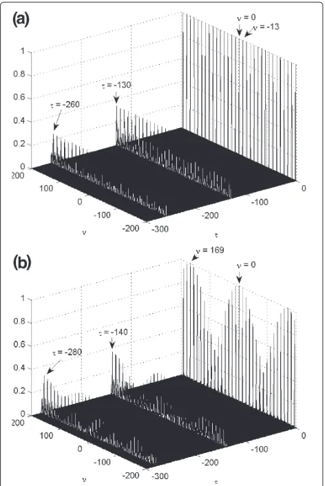
Since|ξ(m)| =1 for allm, we conclude that the AF sur-face is non-zero only whenνis an integer multiple ofM. Therefore, the location of the sidelobes whenn = 0 can also be chosen by adjusting the value ofM. An example of this is shown in Figure 2 that depicts the AF surface of an MCPC CAZAC waveform with = (130, 13, 0); all non-zero sidelobes exist whennis an integer multiple of Q=130.
Positive cyclic frequency-shift
When ζ > 0, we obtain higher diversity in the loca-tions of the AF sidelobes. Specifically, when ζ = 0 in (5), we observe that the terms ej2π((m−n)/Q))qζ /M and e−j2π(m/Q)q˜ζ /Mrepeat multiple times in the summation
in Equation (5). This is due to the summation of these
terms overq=1,. . .,Q−1 and the moduloM/ζeffect of the two exponential functions which is due toM/ζ < Q. Therefore, we can factor the repeating terms and rewrite (5) as
AFs(n,ν) = 1
Es MQ−1
m=0
ξ((m−n)/Q)ej2πmν/(QM)ξ∗(m/Q))
β−1
α=0
ej2π((m−n)/Q)ζ α/M
·
Q/β−1
q=0
e−j2π(βq+α)(m−n)/Q β−1
˜ α=0
e−j2π(m/Q)ζα/˜ M
Q/β−1
˜
q=0
ej2π(βq˜+ ˜α)m/Q. (7)
Note thatqandq˜ now vary from 0 toQ/β −1. We chooseQ,Mandζ such thatβ = (M−1)/ζ +1 is approximately a multiple of Qfor most choices of ζ = 1,. . .,M−1. This eliminates the summation terms forq andq˜ that fall between the values of(β(Q/β −1)+ β−1)andQ−1. These terms were omitted in (7), which explains the use of the approximation symbol, as they only cause a negligible variation of sidelobes in the AF surface compared to the exact expression. The accuracy of the above approximation can be verified using a numerical-based analysis, i.e., the generation of the AF surface using the Matlab code used in this work which is available to the reader upon request. The summation with respect to q˜ can be simplified using q˜Q=/β0−1ej2πqm˜ /(Q/β) = (Q/β) δ(m− ˜m(Q/β)), wherem˜ = 0,. . .,(βM−(β/Q)) is an integer. We then letm = ˆmQ+ ˇm(Q/β), where
ˆ
m = 0,. . .,M − 1 and mˇ = 0,. . .,β − 1. Also, Q/β−1
q=0 ej2πqn/(Q/β)=(Q/β) δ(n− ˜n(Q/β)), wheren˜is
an integer. We letn= ˆnQ+ ˇn(Q/β)withnˆan integer and
ˇ
n=0,. . .,β−1. This simplifies Equation (7) to
AFs(n,ν) = 1
Es Q2 β2
M−1
ˆ
m=0 β−1
ˇ
m=0 ξ(mˆ − ˆn
+(mˇ − ˇn)/β)ej2π(mˆβ+ ˇm)ν/(βM)ξ∗(m)ˆ
· β−1
α=0
ej2π(mˆ−ˆn+(mˇ−ˇn)/β)ζ α)/Me−j2π(mˇ−ˇn)α/β
β−1
˜ α=0
e−j2πmˆζα/˜ Mej2πmˇα/β˜ . (8)
This expression shows that non-zero values of the AF exist fornˆinteger andnˇ=0,. . .,β−1, i.e.,n= ˜nQ/βfor integern. This provides for controlled size valleys in the˜ AF surface.
We also examine what happens along the Doppler axis νat zero delay andζ >0. If we setn= 0 ornˆ = ˇn= 0 in (8), then the termej2π(mˆβ+ ˇm)ν/(βM)reveals that the AF surface As(0,k) has sidelobes that periodically repeat
with periodβM. Evaluating the above expression at the in-between intervals, we can obtain the AF surface side-lobe values. We then choose to use only waveforms with parametersQ,M, andζwith relatively low sidelobe levels in their AF surface withn=0.
Whenζ = 1,β = M, larger valleys appear in the AF surface. Specifically, the AF in (8) becomes:
AFs(n,ν) = 1 Es
Q2 β2
β−1
ˆ m=0
β−1
ˇ m=0
ξ(mˆ − ˆn
+(mˇ − ˇn)/β)ej2π(mˆβ+ ˇm)ν/β2ξ∗(mˆ)
· β−1
α=0
ej2π(mˆ− ˇm−(nˆ−ˇn)+(mˇ−ˇn)/β)α/β
β−1
˜
α=0
e−j2π(mˆ− ˇm)α/β˜ .
Using βα˜−=01e−j2π(mˆ− ˇm)α/β˜ = βδ(mˆ − ˇm) since 0 ≤ ˆ
m ≤ β − 1, 0 ≤ ˇm ≤ β −1 and, therefore, having m= ˆm= ˇmabove expression becomes
AFs(n,ν) = 1 Es
Q2 β2
β−1
m=0
ξ(m− ˆn
+(m− ˇn)/β)ej2π(mβ+m)ν/β2ξ∗(m)
· β−1
α=0
ej2π(−(nˆ−ˇn)+(m−ˇn)/β)α/β.
Then we note that the factor(m− ˇn)/βcan only take the values of 0 ifm= ˇnand−1 ifm<nˇsince bothmand
ˇ
ntake values less thanβ. This implies that non-zero values of the AF surfaceAs(n,ν)only exist at delay locations
such thatnˆ− ˇnornˆ− ˇn+1 are multiples ofβ. For(m−
ˇ
n)/β = −1 which restrictsnˆ− ˇn+1 to be a multiple of β withm < n, and sinceˇ nˇ < M << MQ,M < Qthen indices of the waveform in the AF expression summation are very limited compared to the waveforms’ lengthMQ (i.e.,m< M). Therefore, the case where(m− ˇn)/β = −1 in the AF expression appears in a very small number of additive terms and is omitted in the following analysis. Letting(m− ˇn)/β =0, and usingαβ−=10e−j2π(nˆ−ˇn)α/β = β δ(nˆ− ˇn), we obtain (for details, see [23])
As(n,ν) = AFs(n,ν)
2
≈ 1
Es
Q2
M−1
m=0
ξ(m− ˆn)ej2π(mβ+m)ν/β2
×ξ∗(m) δ(nˆ− ˇn) 2
.
surface appear at intervals ofQ+(Q/M)in the delay. This is demonstrated in the AF surface of the MCPC CAZAC waveform with=(130, 13, 1), as shown in Figure 2b.
In summary, the possibility of choosing the parameters = (Q,M,ζ )of an MCPC CAZAC waveform, and also rotating the entire AF surface by choosing to take the FT of the waveform, enables us to position sidelobes in order to minimize the predicted MSE, as we will show in Section “Adaptive waveform selection ’’.
IP-LPF algorithm Tracking model
We considerLtargets moving in a two-dimensional (2D) plane, where the number of targets is fixed and known. The target dynamics are modeled by a linear, constant velocity model [24] given by
xl,k=Fxl,k−1+vl,k, l=1,. . .,L, k=1,. . .,K, (9)
where xl,k =
xl,kx˙l,kyl,ky˙l,k T is the state vector for
thelth target at timek,T denotes vector transpose,xl,k,
yl,k andx˙l,k, y˙l,k are the position and velocity in
Carte-sian coordinates, respectively, the matrix F is given by
F =[ 1 t 0 0; 0 1 0 0; 0 0 1 t; 0 0 0 1] (with each row in square brackets), t is the time difference between observations, and vl,k is a zero-mean, additive
white Gaussian process with diagonal covariance matrix
Q = diagσx2,σy2,σx˙2,σ˙y2 that models target devia-tions from constant velocity. The model in (9) can be used to determine the kinematic prior probability distribution function pxl,k|xl,k−1
for the lth target. The multitar-get state vector is expressed in terms of the state vectors
of each target as Xk =
xT1,kxT2,k . . .xTL,k
T
. Following [13], we refer to each componentxl,kofXkas a partition.
Since we assume that the targets move independently, the multitarget kinematic prior distribution is given by pXk|Xk−1
=L
l=1p
xl,k|xl,k−1
.
A radar sensor collects information on the range and range rate of the targets in the scene relative to the sen-sor by transmitting pulses and processing the returns after they are reflected by the targets. The return wave-form provides range inwave-formation, in the wave-form of time delays, and range rate information, in the form of fre-quency shifts of the return waveforms relative to the transmitted waveform. Assuming point targets, the range and range rate for partition l at time stepk, relative to the uth sensor, u = 1,. . .,U are given, respectively, by
[11] rl,u,k =
χu−xl,k
2
+ψu−yl,k
2
and ˙rl,u,k =
˙
xl,k
xl,k−χu
+ ˙yl,k
yl,k−ψu
/rl,k, where(χu,ψu)are
the Cartesian coordinates of the location of theuth sen-sor, and theUsensors are assumed to transmit and receive waveforms independently. The discrete time shift value and discrete Doppler shift value at theusensor, due to the
lth target, are given by [11]nl,u,k =round
2rl,u,k/ (c Ts)
and νl,u,k = round−2fc˙rl,u,kTs/(c M)
, respectively, where round (·) transforms the real number to the nearest integer,cis the velocity of propagation in the medium,fc
is the carrier frequency,Tsis the sampling period, andM
is the total number of waveform samples.
Matched filter statistic
At every time stepk, a signals(m),m = 0,. . .,M−1, is simultaneously transmitted from each sensor in different frequency bands to avoid interference. The received signal at theuth sensor after demodulation is a linear combina-tion of the refleccombina-tions from allLtargets, and it is given by
du,k(m)= L
l=1
Al,ks
m−nl,u,k
ej2πmνl,u,k/Me−j2πnl,u,kζc/M
+vu,k(m).
Here, ζc = fcTs is the discrete carrier frequency of
the transmitted waveform. The sum of random complex returns, Al,k, from many different target scatterers on
target l are zero-mean, complex Gaussian with known variance 2σA,l2 and follow the Swerling I model [25]. Each target is assumed to have a different radar cross section (RCS) [26] and thus its return signal has a differ-ent strength that is represdiffer-ented by the variance ofAl,k. It
is also assumed that the return signal strength depends only on the target RCS and not on the distance between the sensor and the target; the distance is compensated for by amplifying returns that arrive later in time. The noise termsvu,k(m),u=1,. . .,U, are assumed to be zero-mean
complex Gaussian with variance 2N0 and independent
for each sensor. The SNR is given by SNR = σA,l2
wEs/N0
[2], wherelwis the index of the weakest target and Esis
the energy of the transmitted waveform from each sensor. When no target is present,du,k(m)=vu,k(m).
At the receiver, the return signal is matched filtered with a signal representing returns fromtargets, at different time shiftsn˜λ,u,kand different frequency shiftsν˜λ,u,k,λ=
1,. . .,. These time-frequency shifts are derived from the belief in target state using a particle filtering approach. The matched filter output is thus given by
˜
yu,k =
Md−1
m=0
du,k(m)
λ=1
s∗m− ˜nλ,u,k
e−j2πmν˜λ,u,k/M
= L
l=1
λ=1
Al,kEsAFs
˜
nλ,u,k−nl,u,k,νl,u,k
−˜νλ,u,k
e−j2πnl,u,kζc/M
+ Md−1
m=0
vu,k(m)
λ=1
s∗m− ˜nλ,u,k
e−j2πmν˜λ,u,k/M,
whereMd > Mshould be large enough to accommodate
a maximum delay in the signal due to a reflection from the target. Moreover,in (10) equals 1 when independently proposing one partition and = Lif particles ofL par-titions are proposed. The matched filter statistic that we will use for estimation isyu,k=y˜u,k2, and it is written in
terms of the AF ofs(m)in Equation (2).
Measurement likelihood
The statistical properties of the matched filter statisticyu,k
depend on the fact thatAl,kandvu,k(m)are independent,
zero-mean, and complex Gaussian. It can be shown that
˜
yu,kin (10) is also complex Gaussian with zero mean and
yu,kis exponentially distributed both under hypothesisH0
(not target is assumed present) and under hypothesisH1
(Ltargets are assumed present). The two hypothesis for-mulation for the measurement likelihood is thus given by
H0:p0yu,k|xk
= 1
2σ02e −yu,k/
2σ2
0
, if no target is present
H1:p1
yu,k|xk
= 1
2σ12e −yu,k/
2σ2
1
, ifLtargets are present (11)
where (see [23] for derivation)
σ02=2N0Es
λ=1
ρ=1
AFs
˜
nλ,u,k− ˜nρ,u,k,ν˜ρ,u,k− ˜νλ,u,k
σ12=2E2s
L
l=1 σA,l2
λ=1
ρ=1
AFs
˜
nλ,u,k−nl,u,k,νl,u,k
−˜νλ,u,k
AF∗sn˜ρ,u,k−nl,u,k,νl,u,k− ˜νρ,u,k
+2N0Es
λ=1
ρ=1
AFsn˜λ,u,k− ˜nρ,u,k,ν˜ρ,u,k− ˜νλ,u,k
.
(12)
When using the MCPC CAZAC waveforms to com-pute the measurement likelihoods in (11), we can reduce the computational complexity by approximating the above variance expressions. In particular, since the AF sidelobes of MCPC CAZAC waveforms are zero at the locations where, according to the belief in target state, the targets are expected to be we can set AFs(n,ν)to be 0 forn=0
andν = 0 in the above expressions. In addition, for the SCPC waveforms the above holds only approximately due to their non-zero, however, very low AF surface sidelobes. Also, using the fact that AFs(0, 0)=1, we can letσA,l2 =σA2
for alll(whereσA2is a nominal value that we choose, since we assume the target strength to be unknown). Based on
this, we can then setσ02=2N0EsLandσ12=2Es2LσA2+
2N0EsLin (12).
Likelihood partition sampling
The highly concentrated AF of a Bj¨orck CAZAC sequence provides a highly concentrated likelihood proposal distri-bution and a high measurement accuracy. However, the proposal process needs to be modified to sample parti-cles from the likelihood instead of the kinematic prior since the former is much more localized than the latter. To achieve this, we use a likelihood particle filter [15], where the importance density depends on the measurements rather than the kinematic prior.
We propose to integrate the use of the likelihood pro-posal with the independent partition (IP) particle filtering [13,14] concept to efficiently propose particles. In the IP, we propose individual partitions of the multitarget state vector, each representing the state of a single target. We then combine the more accurate partition proposals into particles. The IP algorithm is an approximation to the joint multitarget probability density particle filter [14]; the approximation is accurate when the targets are well sepa-rated in the observation space. When targets are close in measurement space, their partitions cannot be indepen-dently proposed as described above. Due to our use of the Bj¨orck CAZAC sequences that have sharply peaked AFs, the measurements can be well approximated as indepen-dent [27]. Our resulting algorithm, the IP-LPF, belongs to the class of sequential partition algorithms [28]. Algo-rithms of this class propose partitions sequentially and then combine them into particles.
Specifically, we first independently evaluate likelihood values at discrete delay-Doppler bins for each partition. Using these values, we create histograms and sample par-tition states. Note that we narrow our bin selection to a region of probability of almost one in the kinematic prior partition sample. This is necessary to ensure a mini-mum number of bins to build the histogram and to ensure that the sample from the measurements is consistent with the kinematic prior. We then evaluate partition weights by combining measurements from the different sensors using the kinematic prior. Using the normalized partition weights, we independently sample values for each parti-tion. We combine the sampled partitions into particles, compute the weights of the particles, and estimate and resample the particles.
one of which can be selected that agrees with the kine-matic prior information. For multiple targets, there are multiple of these circles for each sensor and each target, and multiple intersection points that do not correspond to true coordinate locations. Therefore, the use of three sensors can help clear the ambiguity by providing fewer intersections of three circles. In order to avoid compli-cated geometry, we first process the returns of two sensors and sample Cartesian coordinate target locations using the likelihood. We then weight the sampled locations with measurements from the third sensor. Our method is for a general number of sensors equal or greater than three; in this work, we kept the number of sensors to a minimum of three.
The partitions sampling based on the likelihood is per-formed in two stages. In Stage 1, we utilize information from only two of the sensors in order to propose a prelim-inary set of partitions. This avoids the complex geometry required to sample Cartesian locations from range and range rate information obtained from three or more sen-sors. In Stage 2, we refine our partitions selection by sampling from the preliminary set of partitions created in the first stage using information from all the sensors.
Stage 1: partitions sampling
We start by propagating each state partition without noise. We let λdenote the proposed partition at timek andldenote the partition that represents the true state of thelth target. Assuming that we use a sequential impor-tance resampling particle filter [15], theith state particle,
i = 1,. . .,N, is given byxˇ(λi,k) =
ˇ
x(λi,k),yˇ(λi,k),xˇ˙(λi,k),yˇ˙(λi,k)T =
Fx(λi,k)−1. Usingxˇ(λi,k), we obtain
ˇ
r(λi,u,k) =
χu− ˇx(λi,k)
2
+ψu− ˇy(λi,k)
21/2
.
We want to determine a region of delay-Doppler bins that could contain observations if the true state is xˇ(λi,k). This region is obtained from the spread of the kinematic prior that determines the possible states of partition λ. If we assume for simplicity that the variancesσx2andσy2 of the kinematic prior in the 2D (x,y) dimensions are equal, then with probability of almost one, the proposed particle will fall within 3σxfromxˇ(λi,k) and within 3σyfrom ˇ
y(λi,k). The maximum and minimum possible sampled x andycoordinates will then yield the maximum and min-imum range. That is, if we assume that the target is at angle π/2 with the sensor, thenrmin,(i) λ,u,k, rmax,(i) λ,u,k =
ˇ
rλ(i,u,k) −3√2σx, rˇ(λi,u,k) +3√2σx
. The range would
then increase/decrease by the amount 3√2 σx =
(3σx)2+(3σx)21/2. The delay would also assume
minimum and maximum index values given by
n(min,i) λ,u,k, n(max,i) λ,u,k = 2rmin,(i) λ,u,k/ (c Ts),
2rmax,(i) λ,u,k/ (c Ts)
.
Similarly, the minimum and maximum values can be obtained for the range rate and thus the Doppler
νmin,(i) λ,u,k,νmax,(i) λ,u,k
= −2fc˙rmin,(i) λ,u,kTs/(cM),
−2fc˙rmax,(i) λ,u,kTs/(cM)
,
wherer˙(min,i) λ,u,k = ˇ˙r(λi,u,k) −3√2σx˙andr˙(max,i) λ,u,k = ˇ˙rλ(i,u,k) + 3√2σx˙.
We form all combinations of indices for delay and Doppler that lie within the minimum and maximum delay and Doppler values using
n(ji)
n,λ,u,k = n (i)
min,λ,u,k+jn, jn=0,. . .,J (i) n (13)
νj(i)
ν,λ,u,k = ν
(i)
min,λ,u,k+jν, jν =0,. . .,J (i)
ν , (14)
whereJn(i) = n(max,i) λ,u,k−n (i)
min,λ,u,k andJ (i)
ν = νmax,(i) λ,u,k −
νmin,(i) λ,u,k. Then, we evaluate the matched filter output at each of these values and for sensoru,
y(ji) n,jν,λ,u,k=
Md−1
m=0
du,k(m)s∗
m−n(ji)
n,λ,u,k
e−j2πmν
(i)
jν,λ,u,k/M
2 = L
l=1
Al,kEsAFs
n(ji)
n,λ,u,k−nl,u,k,νl,u,k
− νj(i)
ν,λ,u,k
e−j2πnλ,u,kζc/M
+ Md−1
m=0
vu,k(m)s∗
m−n(ji)
n,λ,u,k
×e−j2πmν (i)
jν,λ,u,k/M
2
. (15)
Note that we have used only one delay-Doppler pair
n(ji)
n,λ,u,k,ν (i) jν,λ,u,k
in the template signal representing a single partitionλ. The single partition likelihood for this delay-Doppler bin is given by:
p(1i)y(ji) n,nν,λ,u,k|n
(i) jn,λ,u,k,ν
(i) jν,λ,u,k
= 1
2σλ2,1e −y(i)
jn,jν,λ,u,k/
2σ2
λ,1
,
if target λpresent
p(0i)y(ji) n,jν,λ,u,k|n
(i) jn,λ,u,k,ν
(i) jν,λ,u,k
= 1
2σλ2,0e −y(i)
jn,jν,λ,u,k/
2σ2
λ,0
,
We evaluate the likelihood ratio for each delay-Doppler bin as
ˇ βj(i)
n,jν,λ,u,k=
p(1i)y(ji) n,jν,λ,u,k|n
(i) jn,λ,u,k,ν
(i) jν,λ,u,k
p(0i)y(ji) n,jν,λ,u,k|n
(i) jn,λ,u,k,ν
(i) jν,λ,u,k
. (17)
We then obtain
ˇ
B(λi,u,k) =
Jn(i)
jn=0
Jν(i)
jν=0
ˇ βj(i)
n,jν,λ,u,k (18)
and the normalized distribution
ˇ
b(ji)
n,jν,λ,u,k = ˇβ
(i) jn,jν,λ,u,k/Bˇ
(i)
λ,u,k, (19)
from which we sample κj(i)
n,u,k, κ (i) jν,u,k ∼ ˇb
(i)
jn,jν,λ,u,k, jn = 0,. . .,Jn(i), jν = 0,. . .,Jν(i), for each particle i and
each sensor u = 1, 2. The resulting sampled range and range rate and the bias are, respectively, rj(i)
n,jν,λ,u,k = c n
(i)
κjn,λ,u,kTs/2, r˙ (i)
jn,jν,λ,u,k = −c Mν
(i) κjν,λ,u,k/
(2fcTs), b(ji)
n,jν,λ,u,k = ˇb
(i)
κjn,κjν,λ,u,k. The values ofr
(i) jn,jν,λ,u,k and r˙(ji)
n,jν,λ,u,k, in turn, yield proposed state values x˜
(i) λ,k.
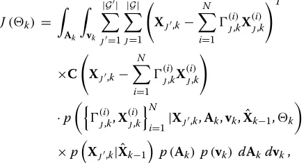
This is accomplished by taking the intersection of two circles in the 2D Cartesian plane and choosing the inter-section point that mostly agrees with the kinematic prior information. This process is illustrated in Figure 3. We note that the sampled partitions x˜(λi,k) from Stage 1 are based on information provided from only two sensors. Therefore, some of these partitions may be incorrect, as previously explained. However, the value of x˜(λi,k) can be used in Stage 2 to evaluate likelihoods for three sensors in order to sample proposal partitions and help remove partitions that have incorrectly been sampled.
Stage 2: partitions sampling
During Stage 1, we propose partitionsx˜(λi,k),i = 1,. . .,N, from delay-Doppler bins associated with sensors u=1, 2. In Stage 2, we utilize the return signals transmitted by U≥3 sensors to refine our choice of partitions and to more accurately represent the target state. We first describe the complexity in calculating the partition weights and the approxi-mation we use to make the computation tractable before we provide the details on the sampling process.
After matched filtering, and using the locations in the delay-Doppler plane derived from the proposed partitions, the measurements from sensorsu = 1,. . .,U are given by
y(λi,u,k) =
Md−1
m=0
du,k(m)s∗
m− ˜n(λi,u,k) e−j2πmν˜λ(i,)u,k/M
2 = L
l=1
Al,kEsAFs
˜
n(λi,u,k) −nl,u,k,νl,u,k
−˜νλ(i,u,k)
e−j2πnl,u,kζc/M
+ Md−1
m=0
vu,k(m)s∗
m− ˜n(λi,u,k) e−j2πmν˜λ(i,)u,k/M
2 , (20) where ˜
n(λi,u,k) , ν˜λ(i,u,k)
is the delay-Doppler pair that
cor-responds to the state x˜(λi,k) and the uth sensor, and
nl,u,k,νl,u,k
is the true target state xl,k. Therefore,
the single partition likelihood function for each pro-posed partition λ of particle i¯ = 1,. . .,N is given by U
u=1p (i¯) λ
y(λi,u,k)
N
i=1|˜x 1 λ,k,. . .,x˜
(i¯)
λ,k,. . .,x˜Nλ,k
. Here, the
hypothesis of particle i¯ and partition λ is that the par-tition state equals x˜(λi¯,k) and not x˜(λi,k) for i = i¯, while
y(λi,u,k) ,i = 1,. . .,N,u = 1,. . .,U are the measurements obtained from matched filters at the delay-Doppler loca-tion defined by the particle proposed target state vectors
˜
x(λi,k),i = 1,. . .,N. However, each likelihood for sensoru is a multivariate exponential distribution [29] that grows in dimensionality as the number of particlesNincreases. We approximate the likelihood for each partition to be U
u=1p (i¯) 1
y(λi¯,u,k) |˜x(λi¯,k)
N i=1,i=i¯p
(i) 0
y(λi,u,k) |˜x(λi,k)
, where
p(1i)
y(λi,u,k) |˜x(λi,k)
denotes the likelihood that a target exists
at x˜(λi,k) andp(0i)
y(λi,u,k) |˜x(λi,k)
denotes the likelihood that a
target does not exist at x˜(λi,k). In [27], we show that the
covariance between measurementsy(λi¯,u,k) andy(λi,u,k) , i¯=i,
depends on the filter proximity (i.e., the closeness ofn˜(λi¯,u,k) ,
˜
νλ(i¯,u,k) andn˜(λi,u,k) ,ν˜λ(i,u,k) ) relative to the AF spread. There-fore, the measurement independence approximation for the Bj¨orck CAZAC is reasonable due to its concentrated AF. Using this approximation, the weights for partitionλ of particle i¯=1,. . .,Nare
˜ βλ,(i¯k) ∝
U u=1p
(i¯) 1
y(λ,i¯u),k|˜x(λ,i¯k)
N i=1,i=i¯p(0i)
y(λ,i)u,k|˜x(λ,i)k
2 u=1b
(i¯) jn,jν,λ,u,k
×p
˜
x(λ,i¯k)|˜x(λ,i¯k)−1
If we divide the right-hand side by the constant U
u=1
N i=1p
(i) 0
y(λi,u,k) |˜x(λi,k)
, and we use (17)–(19), we obtain
˜ βλ(i¯,k)∝
2
u=1 ˇ
B(λi¯,u,k) p(1i¯)
y(λi¯,3,k) |˜x(λi¯,k)
p(0i)
y(λi¯,3,k) |˜x(λi¯,k)
p
˜
x(λi¯,k)|˜x(λi¯,k)−1
,
where the likelihood probability functions are given in (11) for a single target. This is then normalized
˜
bλ(i¯,k)= ˜βλ(,ki¯)/B˜λ,k, (22)
where
˜
Bλ,k = N
i¯=1 ˜
βλ(i¯,k). (23)
We finally perform partition resampling, where we
sam-ple a partition index κ i¯ ∼ ˜b
(i¯)
λ,k, i¯ = 1,. . .,N, from
the distribution of b˜(λi¯,k) with replacement. The resulting
selected partition has value x(λi,k) = ˜x (κ
i¯)
λ,k and selection
probabilityb(λi,k) = ˜b
(κ
i¯) λ,k .
Particle weighting
After partition resampling, we assemble particles from the
sampled partitions asX(ki)=
x(1,ki)T. . .x(L,ki)T
T
. We weigh these particles with weights that incorporate prior and measurement information. To find the weight equation, we start by defining a measurement matrix Yk that is
composed of measurements fromX(ki)and contains mea-surements from each of theUsensors. Specifically,
Yk =
y(u,ki)
, i=1,. . .,N, u=1,. . .,U,
where
y(u,ki) =
Md
m=0
du,k(m)
λ=1
s∗
m−n(λi,u,k)
e−j2πmνλ(i,)u,k/M
2
=
L
l=1
λ=1
Al,kEsAFs
n(λi,u,k) −nl,u,k,νl,u,k
−νλ(i,u,k)
e−j2πnl,u,kζc/M
+ Md
m=0
vu,k(m)
λ=1
s∗
m−τλ(i,u,k)
e−j2πmν(
i) λ,u,k/M
2
.
(24)
Figure 3Schematic of the likelihood proposal process.Each particlexˇλ(i,)k= ˇxnλ,kis deterministically propagated forward (left top figure, arrows 1, 2), the observation points for sensors 1 and 2 are defined (right top and right bottom), one point is sampled from each observation set of each sensor (arrows 3, 4), and one of the two statesx˜(λi,)k= ˜xn
The likelihood function (for a single partition case) for each proposed particle i¯ = 1,. . .,N is given by p(i¯)
y(u,ki)|X1k,. . .,X(ki¯),. . .,XNk
, i = 1,. . .,N, u =
1,. . .,U. Here, the hypothesis of particle i¯ is that the state
equals X(ki¯), while y(u,ki) are the measurements obtained from matched filters at the delay-Doppler location defined by the particle proposed target state vectors X(ki). Note that this likelihood is a multivariate exponential distri-bution [29]. Using similar arguments as for the single partition case, we approximate the likelihood for each
par-ticle to be Uu=1p(1i¯)
y(u,ki¯)|X(ki¯)
N
i=1,i=i¯p(0i)
y(u,ki)|X(ki)
,
wherep(1i)yu,k(i)|X(ki)is the likelihood given that the target
state equalsX(ki)andp(0i)y(ki)|X(ki)is the likelihood given
that no targets exist having stateX(ki).
The weight of particle i¯ [15] using the aforementioned assumptions is given by
w(ki¯) = w(ki¯−)1 U
u=1p (i¯) 1
y(u,ki¯)|X(ki¯)
N
i=1,i=i¯p(0i)
y(u,ki)|X(ki)
λ=1b (i¯) λ,k
×p
X(ki¯)|X(ki¯−)1
.
Dividing by the constantUu=1Ni=1p(0i)
y(u,ki)|X(ki)
, using the likelihood in (11), and normalizing the weights by
Wk=Ni¯=1wki¯, we obtain the normalized weighs
k(i¯)= (i¯) k−1
Wk
U u=1p
(i¯) 1
y(u,ki¯)|X(ki¯)
p
X(ki¯)|X(ki¯−)1
U
u=1p (i¯) 0
y(u,ki¯)|X(ki¯)
λ=1b
(i¯) λ,k
. (25)
The state estimate is thus given byXˆk =
N i¯=1
(i¯) k X
(i¯) k .
The algorithm is outlined next.
IP-LPF algorithm
For each partitionλ=1,. . .,and for each particle
i=1,. . .,N
Stage 1: Likelihood Partition Sampling
✶ Letxˇ(λi,k) =Fx(λi,k)−1
✶ For each sensoru=1,. . .,U
∗ Forjn=0,. . .,Jn(i)and forjν =0,. . .,Jν(i)
♦ Formn(ji)
n,λ,u,kusing (13) andν
(i)
jν,λ,u,kusing (14)
♦ Evaluatey(ji)
n,jν,λ,u,kusing (15) andbˇ
(i)
jn,jν,λ,u,kusing (19)
♦ Sampleκj(i)
n,u,k,κ (i) jν,u,k ∼ ˇb
(i) jn,jν,λ,u,k ♦ Letr(ji)
n,jν,λ,u,k =c n
(i)
κjn,λ,u,kTs/2
♦ Letr˙(ji)
n,jν,λ,u,k = −
cνκ(i)
jν,λ,u,kM
/2fcTs
and
b(ji)
n,jν,λ,u,k = ˇb
(i) κjn,κjν,λ,u,k
✶ Calculatex˜λ(i,k) fromr˜(ji)
n,jν,λ,u,kand˜˙r
(i) jn,jν,λ,u,k
Stage 2: Likelihood Partition Sampling
✶ For each particle i¯=1,. . .,N
∗ Evaluatey(λ¯i,3,k) using (20) andb˜(λ¯i,k)using (22)
∗ Sampleκi
¯∼ ˜b
(¯i) λ,k
✶ Letx(λi,k) = ˜x (κi
¯)
λ,k andb (i) λ,k = ˜b
(κi
¯)
λ,k
Particle Weighting
For each particlei=1,. . .,N
✶ Assemble particlesX(ki)=
x(1,ki) . . .x(L,ki)
✶ EvaluateYk =
y(u,ki)
U
u=1using (24)
✶ For each particle i¯=1,. . .,N
∗ Evaluate particle weights:
(k¯i)=
(¯i)
k−1
Wk
U u=1p
(¯i) 1
y(u,k¯i)|X(k¯i)
p
X(k¯i)|X(k¯i−)1
·1/
U u=1p
(i¯) 0
y(u,k¯i)|X(k¯i)
λ=1b
(¯i) λ,k
EstimateXˆk=Ni
¯=1
(¯i) k X
(i¯) k
Incrementk by 1
Adaptive waveform selection
In order to further improve tracking performance, we adaptively select the parameters of the MCPC CAZAC transmit waveform at each time step k so that we can minimize the predicted tracking root mean-squared error (RMSE). The three MCPC CAZAC parameters we con-sider arek =(Qk,Mk,ζk)in (4), whereQkis the number
of cyclically permuted Bj¨orck CAZAC sequences at time k,Mkis the length of the sequences at timek, andζkis a
parameter that controls the cyclic frequency shift at time k. The expected RMSE is given by the cost function
J(k)=EXˆk,Xk,Ak,vk| ˆXk−1,k
Xk− ˆXk
T
C
Xk− ˆXk
(26)
where the weighting matrix C makes the units of the cost function consistent by compensating for the differing units of the state vector. The subscript in the expecta-tion operatorE·[·] shows the dependance of the expected RMSE on the random target strength vectorAk, the
ran-dom noise matrixvk, the unknown true target stateXk,
and the estimateXˆk, given the multitarget state estimate ˆ
Xk−1atk−1 and the choice ofk.
Next, we identify the set of values that the multitar-get state estimate Xˆk can take in terms of the
we have considered a discrete finite set of delay-Doppler locations for each partition and each particle. This set cor-responds to Cartesian coordinate locations that are most likely to occur according to the kinematic prior and the set of particlesX(ki−)1, i = 1,. . .,N generated at the pre-vious time stepk −1. The set is given in (13) and (14) asn(ji)
n,λ,u,k,ν (i) jν,λ,u,k
,jν = 0,. . .,Jν(i)andjn = 0,. . .,Jn(i),
forλ = 1,. . .,,u = 1,. . ., 2 andi = 1,. . .,N. We use indexj to denote a member of the setG, of cardinality
|G|, consisting of the N particles that could be sam-pled by the IP-LPF proposal and subsequently weighted. Therefore,G is a large set including all combinations of possible delay-Doppler locations from two of the sensors for each target and particle. The process of forming par-titions from sampled delay-Doppler locations is explained in Section “Stage 1: partitions sampling” and illustrated in Figure 3. Subsequently, one possible outcome of the likeli-hood sampling process and particle weighting isN weight-particle pairs
j(i,k),X(ji,k)
,n=1,. . .,Ncorresponding to
delay-Doppler locations
n(ji,)λ,u,k,νj(i,)λ,u,k
,λ = 1,. . .,, u =1,. . .,U,i= 1,. . .,N. Similarly, based on the target motion model, we can identify a discrete finite set of pos-sible true target statesXk. Each possible true target state
Xj,k with index j is a member of the set G, of
cardi-nality|G|.Xj,kis related to corresponding delay-Doppler
locationsnj,l,u,k,νj,l,u,k
,l=1,. . .,L,u=1,. . .,U. From the above, we may rewrite the cost function in (26) as
J(k) =
Ak
vk
|G|
j=1 |G|
j=1
Xj,k−
N
i=1
(ji,k)X(ji,k)
T
×C
Xj,k−
N
i=1
j(i,k)X(ji,k)
·p
(ji,k),X(ji,k)
N
i=1|Xj,k,Ak,vk,Xˆk−1,k
×pXj,k| ˆXk−1
p(Ak) p(vk) dAkdvk,
where the probability distributions p
Xj,k| ˆXk−1
, p(Ak), andp(vk)are defined in the context of the motion
and measurement models in Sections “Tracking model” and “Matched filter statistic”.
In order to minimize the cost function, we need to minimize the probability
p
(ji,k),X(ji,k)N
i=1|Xj,k,Ak,vk,Xˆk−1,k
and the
par-ticle weights j(i,k) in (25) for particles (i) such that
Xj,k =X(ji,k). As thejth set of particles
X(ji,k)
N
i=1results
from sampling by the IP-LPF, we will follow the sam-pling process of the IP-LPF and identify the selection
probability for each partition of particles
X(ji,k)
N
i=1.
According to Section “Stage 1: partitions sampling”, we obtain values x˜(λi,k) for each partition λ = 1,. . .,and each particlei=1,. . .,Nby sampling delay-Doppler bins from sensors u = 1, 2 with probability 2u=1b(ji)
n,jν,λ,u,k given by (19). The values x˜(λi,k) allow us to evaluate the likelihoods for the U sensors in order to sample par-titions. In Section “Stage 2: partitions sampling”, we obtain partitions x(λi,k) with selection probability b(λi,k) given by (22). These sampled partitions are combined into particles into particles X(ki) in Section “Particle weighting”. From the sampling process of each particle
X(ki), we conclude that the probability of each particle being selected isλ=1b(ji,)λ,k2u=1b(ji,j)
n,jν,λ,u,k. Therefore, any set of particles X(ji,k)N
i=1 appears with
probabil-ity p
(ji,k),X(ji,k)N
i=1|Xk,Ak,vk,
X(ki−)1N
i=1,k
=
N i=1
λ=1b (i) j,λ,k
2 u=1b
(i)
j,jn,jν,λ,u,k. Furthermore, from (21), (22), forb(ji,)λ,k and from (17), (19) forb(ji,j)
n,jν,λ,u,k we observe that the above sampling probabilities depend on the single partition likelihood ratio which using (16) is
proportional to exp
σλ2,1−σλ2,0 2σλ2,1σλ2,0
N
i=1
U
u=1y (i) j,λ,u,k
. Since
σλ2,0 < σλ2,1, the selection probability monotonically
increases with the matched filter statisticy(ji,)λ,u,k. There-fore, in order to minimize the above selection probability the matched filter statistic needs to be minimized for the delay-Doppler values in (13) and (14) with the additional constraint thatn(ji,)λ,u,k = nj,l,u,k,νj,l,u,k = νj(i,)λ,u,k for all
partitionsλ, particlesiand sensorsu. These sets of delay-Doppler locations correspond to the belief on target state as explained previously and only include delay-Doppler locations that imply erroneous target statesXj,k = X(ji,k)
(i.e., AF sidelobes). Since the matched filter statistic is a random variable it is minimized by minimizing its variance, given in (12) with = 1, with respect to the waveform parameters.
Next, we observe that the particle weightsj(i,k) in (25) contain the likelihood ratio both in the numerator and denominator. This, together with the fact that the prior has a wide spread compared to the likelihood, makes the particle weights nearly constant. Therefore, particle weights cannot be significantly reduced by adjusting the waveform parameters.
Therefore, the focus is on minimizing the matched fil-ter statistic variance in (12) with respect to the waveform parameters specifically for the delay-Doppler values in (13) and (14) and such thatn(ji,)λ,u,k = nj,l,u,k,νj,l,u,k =