New algorithm for mode shape estimation based on ambient signals considering model order selection

R E S E A R C H

Open Access

New algorithm for mode shape estimation based

on ambient signals considering model order

selection

Chao Wu

, Chao Lu

and Yingduo Han

Abstract

Using time-synchronized phasor measurements, a new signal processing approach for estimating the

electromechanical mode shape properties from ambient signals is proposed. In this method, Bayesian information criterion and the ARMA(2n,2n–1) modeling procedure are first used to automatically select the optimal model order, and the auto regressive moving averaging models are built based on ambient data, then the low-frequency oscillation modal frequency and damping ratio are identified. Next, Prony models of ambient signals are presented, and the mode shape information of multiple dominant interarea oscillation modes are simultaneously estimated. The advantages of the new ARMA-P method are demonstrated by its applications in both a simulation system and measured data from China Southern Power Grid.

Keywords:Electromechanical dynamics, Mode shape, Ambient signal, Model order selection, ARMA-P method

Introduction

Modal frequency, modal damping ratio, mode shape magnitude, and mode shape angle are the key para-meters describing the electromechanical modal prop-erties of a power system [1]. Similar to former two, the mode shape properties that describe the participa-tion of state variables in a particular mode are of vital importance for the safety and reliable operation of the system. Near real-time knowledge of mode shape characteristics provide critical information for the optimization of generators and/or load shedding, in order to improve the damping of the dangerously low-damped modes of power systems.

In general, the analysis of mode shape properties can be accomplished using two basic approaches: the eigen-analysis of a small signal model [1], or as shown in this article, signal processing of the time-synchronized mea-surements. One important advantage of the signal-based method is that the identification is dependent on the large, complex system model. In this category, the Prony method [2,3] and the Eigensystem Realization Algorithm

[4,5] are widely used. However, their applications are generally limited only for ringdown signals, which are relatively few in actual power grids. Ambient signals, caused by low-level stochastic disturbances, are more frequently and easily collected in real systems. Some publications have offered algorithms for identifying the modal frequency and damping ratio from ambient data [6-9], which fully demonstrate that this kind of signal includes abundant information about the system. Only recently the mode shape has been considered [10-14]. Based on the relationship between the cross- and power spectral densities and mode shapes, an approach for es-timating the mode shapes using spectral method is pre-sented in [10]. Liu and Venkarasubramanian [11] applied the frequency domain decomposition method to the mode shape identification. Then, the channel matching method was introduced in [12] and refined in [13], in which a narrowband bandpass filter must firstly be used to extract one single mode from multiple modes. In this case, the changes of operation modes in actual power system would inevitably cause the ineffect-iveness of the prefixed filter, and influence the estima-tion accuracy. In [14], the transfer funcestima-tion method was proposed which showed that mode shape could be cal-culated by evaluating a transfer function, constructed

* Correspondence:wuchao@szu.edu.cn

1

College of Mechatronics and Control Engineering, Shenzhen University, Shenzhen 518060, China

Full list of author information is available at the end of the article

between a pair of system outputs, at the mode of inter-est. However, as the key factors of transfer function, the selection of model order are not taken into account in these articles, this will directly affect the accuracy of the mode shape analysis results.

In this article, in order to identify the low-frequency oscillation mode shape properties based on ambient sig-nals, a new multiple modes estimation method called the auto regressive moving averaging-Prony (ARMA-P) is proposed. In addition, the problem of optimal model order selection in ARMA modeling is considered, which would improve the efficiency and accuracy of the new ARMA-P method.

The remainder of this article is organized as fol-lows. Section 2 describes the feasibility and the the-oretical basis of using the ARMA and Prony models together to extract the mode shapes from ambient data. In Section 3, different model order selection criteria are comparatively discussed, and ARMA (2n,2n – 1) modeling procedures are adopted to optimize the order selection path. To estimate the mode shape characteristics based on ambient signals, the equations of ARMA-P method are derived in Section 4. Sections 5 and 6 provide the simulation and actual system examples, respectively. The results demonstrate that the new ARMA-P method can ef-fectively estimate the mode shape properties from ambient data. Conclusions are provided in Section 7.

Theoretical basis of ARMA-P method

It is well known that under small-signal disturbance conditions, the power system may be linearized and represented in state space form [1],

_ x tð Þ ¼A

x tð ÞþB

q tð Þ ð1Þ

where x is the n× 1 system state vector, including ma-chine rotor angles and velocities. Input vector q (order

m× 1) is a hypothetical random-noise source vector per-turbing the system. Under ambient conditions, inputqis typically conceptualized as noises produced by random loads switching in power systems.A(ordern×n) is the state matrix and B (order n × m) is the input matrix. Measurement-based electromechanical mode estimation assumes that the power system is in the steady-state condition described by (1).

It has been well established that the eigensolution of the state matrix Ain (1) provides all the required infor-mation to completely describe the modal properties of power system. The reader can refer to [1] for more de-tail. A brief review of these properties is described here.

The eigenvalues and eigenvectors associated withAare

λkIA

j j ¼0 ð2aÞ

A u

k¼λkuk ð2bÞ

vkA¼λkvk ð2cÞ

where λk is the kth eigenvalue (k = 1. . .n), uk = [u1,k, u2,k, . . . un,k]T is the kth right eigenvector, vk = [vk,1, vk,2, . . .vk,n] is the kth left eigenvector.

Then the linear transformation defined in (3) is ap-plied to the system (1), and the system state xiis calcu-lated, shown in (4).

x1

⋮

xn 2 4

3

5_¼ u_⋮1;1 . . ._⋱ u_⋮1;n

un;1 . . . un;n 2

4

3

5 zM1

zn 2 4

3

5 _ð3Þ

xi¼

Xn

k¼1

ui;keλkt zkð Þ þ0 Xn

l¼1 Xm

j¼1

νk;lbl;j Z t

0

eλkτ_qð Þτ _dτ

" #

( )

ð4Þ

wherebl,j is thelth rowjth column element in the input matrixB,zl(0) is the initial value ofzk.

Equation (4) provides information on how the modes are combined to create the system states. The element

ui,k (the ith element of uk) provides critical information on how the ith state (generators and other dynamic devices) participates in the kth oscillation mode. The magnitude of ui,k determines the intensity level for the state variable xi to participate thekth oscillation mode, and the angle ofui,kdetermines the oscillation phase of the state variablexiin thekth oscillation mode.

Thus, comparing the elements ui,k and uj,k describes the mode shape information between statesi andj. The mode shape magnitude is then defined as the ratio of the magnitudes ofui,kanduj,k

Magnitude¼ ui;k

uj;k

ð5Þ

and the mode shape angle is the difference between the angles ofui,kanduj,k

Angle¼∠ui;k∠uj;k ð6Þ

Then rewrite (4) as

xið Þ ¼t

Xn

k¼1

Φi;kð Þt eλkt ð7Þ

where

Φi;kð Þ ¼t ui;k zkð Þ þ0

Xn

l¼1

Xm

j¼1 νk;lbl;j

Z t

0

eλkτ_qð Þτ _dτ

" #

ð8Þ

weighted exponential components to fit the sampled sig-nal, Prony model is adopted to describe the approximate signal as follows

^xið Þ ¼κ

Xn

k¼1

Ψi;kð Þκ eλkTκ ¼

Xn

l¼1

Ai;kejθi;keðαkþj2πfkÞTκ

ð9Þ

where κ = 0,1. . .N – 1, N is the data length, n is the number of oscillation modes.

Each term in (9) has four elements: the damping factor

αk, the frequencyfk, the magnitudeAi,k, and the angleθi,k. Each exponential component with a different frequency is viewed as one unique mode of the original signal.

From (7) and (9), it can be deduced that on the sample point

Xn

k¼1

Φi;kð ÞκT eλkTκ¼

Xn

k¼1

Ψi;kð Þκ eλkTκ ð10Þ

Obviously

Ψi;kð Þ ¼κ Φi;kð ÞκT ð11Þ

Taking (8) into consideration, Ψi,k is time-varying, defined as

Ψi;kð Þ ¼κ Ψi;k0þΔΨi;kð Þκ ð12Þ

where

Ψi;k0¼ui;kzkð Þ0 ð13aÞ

ΔΨi;kð Þ ¼κ ui;k

Xn

l¼1

Xm

j¼1 νk;lbl;j

Z t

0

eλkτ_qð Þτ _dτ ð_13bÞ

It can easily be found that Ψi,k0is time-invarying, and it is proportional to the right eigenvectors ui,k with a constant zk(0), whereas ΔΨi,k(κ) is time-varying due to the change of the input vectorq.

Thus, considering (5), (6), and (13a), the mode shape information of kth oscillation mode between the signals

iandjcan be estimated by

Magnitude¼ ui;k

uj;k

¼ Ψi;k0

Ψj;k0

ð14aÞ

Angle¼∠ui;k∠uj;k¼∠Ψi;k0∠Ψj;k0 ð14bÞ

Assuming for the moment that all signals are time-synchronized samples, and a reference state or signal is chosen as the state having the high observability in the

kth oscillation mode, the theoretical feasibility of ARMA-P method estimating mode shape properties of multiple modes based on ambient signals is certified.

Model order selection

In the ARMA modeling of ambient signal, the model order selection is an important step. The applicability of model order will influence the accuracy and efficiency of oscilla-tion modal frequency and damping ratio analysis, and fur-ther affect the mode shapes identification. In addition, the mode shape characteristics are relevant to multiple nodes in power grids, that is to say, we have to build the ARMA models of multiple signals. Obviously, it is time-consum-ing. And for the online application of ARMA-P method, it is best to automatically select the model order. Therefore, the model order selection is studied in this section. Differ-ent model order selection criteria are comparatively dis-cussed, and the modeling procedure is considered to improve the calculation efficiency.

Model order selection criteria

Model order is a key factor in the ARMA model of am-bient signal. A model with too high an order will include too much irrelevant oscillation information, and a model with too low an order may not include enough essential information about the system. Only, the ARMA model, with an optimal model order, can precisely describe the dynamic characteristics of power grids.

Information criteria (IC), which are generally used to determine the model order, are referred to as penalized log-likelihood criteria where the penalized term depends on the number of free parameters in the model and/or the number of observations [15]. They can be written in a generalized form

ICð Þ ¼ p 2X N

i¼1

logf xi^θp

þpC Nð Þ

ð15Þ

wheref(xi|θk),i= 1,. . .,Ndescribes the conditional prob-ability density of the observations x1,. . .,xN, C(N) is an increasing function of the observations numberN, ^θp is the estimator for the unknown model parameter based on the observations, and the optimal order choice is such that^p =argmin IC(p).

Obviously that the second term grows as the para-meters becomes complex, while the first term has the opposite variation, so the minimization of IC realizes a compromise between the data fitting and the complexity of the chosen parameter.

For the model order selection, the most known criter-ion is surely the Akaike’s information criterion (AIC) [16], written as follows

AICð Þ ¼ p 2X N

i¼1

logf xi^θp

þ2p

ð16Þ

since it asymptotically leads to a strictly positive over parameterization probability of the model order [17].

In order to overcome the inconsistency of AIC, Schwarz [18] suggests the widely known Bayesian information cri-terion (BIC) based on the Bayesian justification

BICð Þ ¼ p 2X N

i¼1

logf xi^θp

þplogN

ð17Þ

And a different approach was introduced by Rissanen [19]. This approach suggested using the minimization of the length of a code. This code is required to encode observations. This criterion is referred to as minimum description length (MDL), defines as

MDLð Þ ¼ p 2X N

i¼1

logfxi^θp

þplogN

þðpþ2Þlogðpþ2Þ ð18Þ

Theoretical research has found that BIC and MDL cri-teria are almost surely convergent in that they help in finding the appropriate model order when the observa-tions numberN→∞(strong consistency) and penalized the term of likelihood more than AIC [15]. Because of the similarity of the two criteria, we choose to discuss the performance of BIC in this article.

Another strongly consistent criterion, referred to as ϕ_β, was introduced by El and Hallin [20]. It is a generalization of Rissanen’s work on stochastic complexity [21], written as follows

ϕβð Þ ¼ p 2

XN

i¼1

logf xi^θp

þpNβlog logN

ð19Þ

with the refined conditions shown in (20) [18], which allows for β to be adjusted according to the number of observationsN.

0< log logN logN ≤β≤1

log logN

logN <1 ð20Þ

In this article, we proposed to apply AIC, BIC, andϕ_β, to the estimation of the order of ARMA models shown in (21).

ARMA model is a representative with the assumption that the input is approximately white over the frequency band of interest [22], and it is applicable to describe the characteristics of ambient signals in power grids.

xið Þ ¼κ ς1xiðκ1Þ þ⋯þςnxiðκnÞ φ1aðκ1Þ ⋯φmaðκmÞ

það Þκ ð21Þ

wherea(κ) is the stochastic disturbance input,ςh(h =1. . .n) and φg (g = 1. . .m) are the coefficients of AR and MA parts,Nis the observations number,κ=1. . .N.

The orderpin the criteria above is defined asp=n+m. Omitting terms that do not depend on the model orderp, it is well known that the first terms in these formulae be-come Nlog σ^_a2, where σ^a is the variance estimate of dis-turbance inputashown in (21). Thus, we obtain

ICð Þ ¼p Nlogσ^_a2þpC Nð Þ ð22aÞ

AICð Þ ¼p Nlog^σ_a2þ2p ð22bÞ

BICð Þ ¼p Nlog^σ_a2þ2 logN ð22cÞ

ϕβð Þ ¼p Nlog^σa

2_þkNβ_{log logN ð22dÞ}

The selected model order verifies^p =argmin IC(p).

ARMA(2n,2n–1) modeling procedure

One immediate disadvantage of using the model order selection criterion is that since it is aimed at finding the optimal order among optional items. That is to say, a great many of ARMA models with different orders have to be built first. Obviously, it is time consuming and not good for the online application of the new ARMA-P method. In order to improve the calculation efficiency, the modeling procedure that specifies the search path of the optimal model order is considered in this article.

The ARMA(2n,2n–1) modeling procedure proposed by Wu and Pandit [23] is employed. In this approach, first the ARMA(2n,2n – 1) model with the initial value n = 1 is modeled, then let n = n + 1. Only when the order is ad-equate as judged by the model order selection criterion, this step stops. Following that, the order of the AR and MA parts are reduced, respectively, and the model order selection criterion is applied until the optimal order is found. As shown in Figure 1, comparing with the trad-itional box modeling procedure, the computation efficiency is highly improved using the ARMA(2n,2n–1) modeling procedure. It is better for the online application of the ARMA-P method in identifying the mode shape properties in interconnected power grids.

ARMA-P algorithms

Based on the theoretical deduction of the ARMA-P method in Section 2, the equations of this new approach for extracting the mode shape information from ambient signals are derived in this section.

Estimating the oscillation modal frequency and damping by ARMA model

power grids. This kind of disturbance is assumed to rela-tively be statistically stationary for a block of data over the frequencies of interest [22,24].

The ARMA model of ambient signalxiis shown in (21). First, the optimal model order is selected using IC and the ARMA(2n,2n– 1) modeling procedure. Then when

k = m +1, m +2. . .m + M(M > n), a matrix equation is formed as follows

Rmþ1 Rmþ2

⋮

RmþM 2 6 6 4

3 7 7

5¼

Rm Rm1 ⋯ Rmnþ1 Rmþ1 Rm ⋯ Rmnþ2

⋮ ⋮ ⋮ ⋮

RmþM1 RmþM2 ⋯ RmþMn 2

6 6 4

3 7 7 5

ς1

ς2

⋮

ςn 2 6 6 4

3 7 7 5

ð23Þ whereRkis the autocorrelation function of signalxi.

Rk¼ 1

N

XN

l¼kþ1

xið Þl xiðlkÞ

Equation (23) is called the Modified Yule-Walker equation. The solution of (23) is the estimated coeffi-cient vector of AR part.

A new time series yi(κ) is defined based on the infor-mation of the observationsx1,. . .xNand the AR part co-efficient estimation^ς1;. . .^ςn.

yið Þ ¼κ xið Þ κ ^ς1xiðκ1Þ ⋯^ςnxiðκnÞ ð24Þ And

yið Þ ¼κ að Þ κ φ1aðκ1Þ ⋯φmaðκmÞ ð25Þ And the spectral density function ofyiis calculated

Syiyið Þ ¼ω σ 2

aφð ÞB

2

B¼eiωT ¼σ2 a

Ym

j¼1

1η_i;jB

2

B¼eiωT

ð26Þ whereφ(B) is the polynomial of MA part,Bis the back-ward operator, andTis the sample time.

Obviously whenB =1/ηi,j, (26) equals to zero.

On the other hand, based on the definition of spectral density, the spectral density function of the signal yi is obtained

Syiyið Þ ¼ω

Xm

k¼0

Ryi;kBkjB¼eiωT ð27Þ

whereRyi,kis the autocorrelation function ofyi. Deduced from (26) and (27), we obtained

Xm

k¼0 Ryi;k

1

ηi;j

!k

¼0 ð28Þ

Thenηi,jare calculated from (28), and substituted into the MA polynomial.

Ym

j¼1

1η_i;jB

¼1X

m

j¼1

φjBj ð29Þ

By comparing the homogenous exponential coeffi-cients of operator in (29), the coefficoeffi-cients of MA part are obtained. Thus, the ARMA model of ambient signal is built up.

The conjugate eigenvalues λk, λk* can be calculated by solving the AR polynomial. And the low-frequency oscillation modal frequency fk and damping ratio ξk are calculated

fk¼

ffiffiffiffiffiffiffiffiffiffiffiffiffiffiffiffiffiffiffi lnλklnλk p

2πT :

ffiffiffiffiffiffiffiffiffiffiffiffiffi 1ξ2_k q

ξk¼

lnj jλk ffiffiffiffiffiffiffiffiffiffiffiffiffiffiffiffiffiffiffi

lnλklnλk p

8 > > < > >

: ð30Þ

where k = 1. . .nd, nd is the number of dominant oscil-lation modes.

AR order

1 2 3 4 5 6

1 2 3 4 5

0

MA order

MA order

AR order

0 _{1 2 3 4 5}

1 2 3 4 5

6 (a) ARMA(2n,2n-1) modeling procedure (b) Box modeling procedure

Estimating the mode shape magnitude and angle by Prony model

The approach of Prony model to estimate the electromech-anical properties of power grids can be broken down into two parts [2,3]: first, calculating the eigenvalues of discrete model for estimating the modal frequency and damping ratio; second, computing the weights or coefficients to fur-ther extract the mode shapes properties.

In this part, the dominant oscillation modes, which play important roles in describing the dynamic characteristics of power system, are primarily studied. In general, the en-ergies of the dominant modes take up large proportions in ambient signals. So in this case, the rest modes can be

omitted in this article. Moreover, since the eigenvalues cor-responding to one oscillation mode are conjugate, in the following part only the complex pair eigenvalues are con-sidered. Consequently, based on the dominant modal in-formation shown in (30), the eigenvalues of discrete model in Prony algorithm are calculated as

γk;γk¼ exp 2πfk ffiffiffiffiffiffiffiffiffiffiffiffiffiξk 1ξ2_k

q j2πfk

0 B @

1 C

AT

2 6 4

3 7

5 ð31Þ

wherek =1. . .nd,ndis the number of dominant oscillation modes.

1 1 1

2 1 2 2

1

m m m n

m m m n

m M m M m n

R R R

R R R

R R R

, ,

1 1 1

ˆ =

p p p

l l l l l l

l l l

x z z z

* 2

* ln ln

1 2

ln | |

ln ln

l l

l l

l l

l l

f

T

*

2

, exp ( 2 2 )

1

l

l l

l l

l

f j f T

*

1 1

1 1

( ) ( ) ( )

d d

n n

l l

l l

p p

p

z z z

z a z a 1

( ) (0 )

ˆ ( )

ˆ ( ) ( 1)

i p i

l i

l

x p

x

a x l p N

0 ˆ

i i xi

, , 0

, , 0

i k i k

j k j k

u Magnitude

u

, , , 0 , 0

i k j k i k j k

Angle u u

And the characteristic polynomial of discrete model is built

φð Þ ¼z Y nd

l¼1

zγ_l

_:Ynd

l¼1

zγ_l

¼zp_þa

1zp1þ. . .þap

ð32Þ

Then the coefficients al (l = 1. . .p, p = 2×nd) are obtained from (32).

Following that, the approximate signal^xis calculated

^xið Þ ¼κ

xið Þκ ð0≤κ≤pÞ

X

p

l¼1

al^xiðκlÞðp<κ≤N1Þ 8

> < >

: ð33Þ

In Prony algorithm, the signal^xi is used to fit the true signal xi. Following its principle shown in (9) and (12), the approximate signal^xican be described as

^xið Þ ¼κ

Xp

l¼1

Ψi;lγlκ¼

Xp

l¼1

Ψi;l0γlκþ

Xp

l¼1

ΔΨi;lð Þκ γlκ

ð34Þ

Defining an itemεias follows

εið Þ ¼κ

Xp

l¼1

ΔΨi;lð Þκ γlκ ð35Þ

Considering (13b), the item εi is a weighted sum of disturbance inputs. In this article, the inputs are assumed to relatively be statistically stationary over the frequencies of interest, so the itemεican also be termed as relatively statistically stationary.

Then a matrix equation is created.

1 . . . 1 γ1

1 . . . γ1p

⋮ . . . ⋮

γN1

1 . . . γNp1

2 6 6 4

3 7 7 5

Ψi;10 Ψi;20

⋮

Ψi;p0

2 6 6 4

3 7 7 5þ

εið Þ0 εið Þ1

⋮ εiðN1Þ

2 6 6 4

3 7 7 5¼

^ xið Þ0 ^ xið Þ1

⋮ ^ xiðN1Þ

2 6 6 4

3 7 7 5

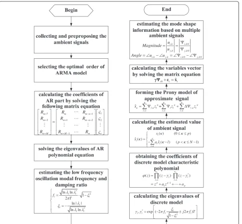
ð36Þ It is rewritten in short as

γΨi0þεi¼^xi

A least square solution of (36) yields the variables vec-tor as shown in (37).

^

Ψi0¼ γTγ

1

γT^x

i ð37Þ

~

~

~

~

~

~

~

~

BUS1 BUS24

BUS25

BUS11

BUS51

BUS9

BUS20

BUS14

BUS21 BUS19

BUS4 BUS23

BUS2

BUS22

BUS3

BUS30

BUS7

BUS31

BUS8

BUS33 BUS5

BUS18

BUS16

BUS50 BUS34

BUS11

BUS29 BUS26

BUS52 BUS12

BUS27 BUS28

BUS6

BUS13

Thus, the mode shape magnitude and angle informa-tion of multiple dominant interarea modes in power grids can be estimated from the variables Ψ^i0 according

to (14).

Therefore, based on ambient signals synchronously collected from power grids, following these steps shown in Figure 2, the system’s mode shape properties are identified.

Simulation examples

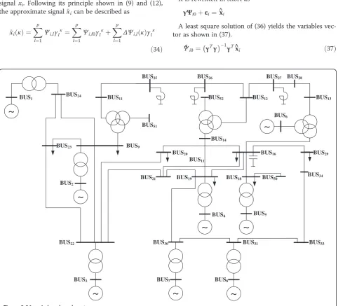
A 36-node benchmark system shown in Figure 3 is used to demonstrate the performance of the ARMA-P method, using the Power System Analysis Software Package as the simulation tool. The system contains eight generators at major generation buses 1 through 8. The generators are represented using detailed two-axis transient models. Each load in this system is split into a portion consisting of constant power and random power. The random portion of both the real and reactive loads is obtained by passing independent Gaussian white noise through low pass filters.

The dominant interarea low-frequency oscillation modes shown in Table 1 are calculated by conducting an eigenalaysis of the entire system’s small-signal model under nominal steady-state operating conditions.

In this article, Mode I (0.778 Hz, 1.123%) is mainly discussed. The mode shape magnitude and angle infor-mation of this mode is given in Table 2. Taking Gen8 as the reference, the eight generators in 36-node bench-mark systems can be classified into two groups: Group A (including Gen1, Gen2), Group B (including Gen3, Gen4, Gen5, Gen6, Gen7, and Gen8). Among them, Gen1, Gen7, and Gen8 have high degrees of participa-tion in Mode I.

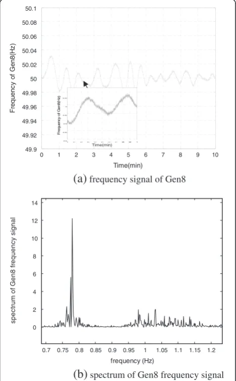
For the examples that follow, a typical time-domain simulation is comprised of driving the sys-tem with random load variations. The syssys-tem’s responses consist of small random variations in the system states. As an example, Figure 4a describes the resulting random variations of Gen8 frequency signal for a 10-min simulation. The spectrum of this signal shown in Figure 4b illustrates that the ambi-ent signal includes rich information about the dom-inant oscillation modes in 36-node benchmark system, especially Mode I.

ARMA-P method is applied to estimate the mode shape properties from the frequency signals of the eight generators in the simulation system. First, these ambient signals are preprocessed. Considering the frequency range of electromechanical mode (generally

0 1 2 3 4 5 6 7 8 9 10 49.9

49.92 49.94 49.96 49.98 50 50.02 50.04 50.06 50.08 50.1

Time(min)

F

requenc

y

of

G

en8(

H

z

)

(a)

0.7 0.75 0.8 0.85 0.9 0.95 1 1.05 1.1 1.15 1.2 0

2 4 6 8 10 12 14

frequency (Hz)

spect

rum

of

G

e

n8 f

requenc

y si

gnal

(b)

49.98 49.985 49.99 49.995 50 50.005

Time(min)

F

reque

nc

y

of

G

e

n

8

(H

z

)

6.8 6.9 7

Figure 4Frequency signal of Gen8 in 36-node benchmark system. (a)Frequency signal of Gen8.(b)Spectrum of Gen8 frequency signal.

Table 2 Mode shape information of mode I in 36-node benchmark system

Gen Magnitude (p.u.) Angle (rad)

1 0.683 3.156

2 0.120 3.076

3 0.474 6.096

4 0.425 −0.050

5 0.597 6.140

6 0.426 −0.067

7 0.983 0.016

Table 1 Dominant low-frequency oscillation modes of 36-node benchmark system

Mode Eigenvalue Frequency (Hz) Damping ratio (%)

[0.1 Hz, 2.5 Hz]) in power systems, the signals are low pass filtered with a cutoff frequency of 3 Hz, then decimated from 50 samples per second to 5 samples per second, and finally high pass filtered to remove any low-frequency trends.

Then according to the procedure of ARMA-P method shown in Figure 2, the model order must be determined first. In order to fully compare the performances of the three typical criteria in power grids, AIC, BIC, and ϕβ are, respectively, applied to select the optimal order of ARMA model based on the simulative ambient data. And the ARMA (2n,2n – 1) modeling procedure is employed to specify the search path.

In this part, the frequency signal of Gen8, which includes rich information about the dynamic characteris-tic of system, is chosen to be the analysis object. The number of observations isN= 3000. According to (20), the bounds on the valueβinϕβcriterion are calculated,

βmin= 0.2598,βmax= 0.7402. So in this case, the ϕβ cri-terion has been calculated for values of β equal to 0.3, 0.4, and 0.5.

The research on the model order selection is based on 50 experiments. The eigenvalues results of different model order selection criteria are plotted in Figure 5, and the average value of the order for the 50 experi-ments is given in Table 3. The oscillation mode proper-ties in each case are also calculated.

We can notice that AIC leads to over-parameterization whileϕ_β(β=0.4, 0.5) under-parameterize because of the high penalty. The order results of BIC andϕ_β(β=0.3) are similar. Considering the relatively limited system dy-namic information that include in ambient data, a small change in model order would lead to a large variation in estimated modal parameters and influ-ence the identification accuracy. So, the oscillation mode characteristic results corresponding to BIC and ϕ_β (β = 0.3) are further compared, in order to discuss the applicability of these criteria in power systems. Comparing with the eigenanalysis results shown in Table 1, the accuracy of the modal infor-mation corresponding to BIC are much better. Con-sidering Occam’s Razor [25], BIC is appropriate to select the optimal order of ARMA model, and its feasibility is testified.

Table 4 Analysis results of Mode I based on frequency signals of eight generators

Gen Frequency (Hz) Damping ratio (%)

1 0.778 0.995

2 0.774 2.014

3 0.772 1.331

4 0.771 1.566

5 0.775 1.136

6 0.779 1.400

7 0.775 1.341

8 0.776 1.270

Table 3 Oscillation modes results of three typical model order selection criteria

Criterion Model

order

Mode I Mode II

Frequency (Hz)

Damping ratio (%)

Frequency (Hz)

Damping ratio (%)

AIC (16,15) 0.774 1.702 0.959 4.905 BIC (12,11) 0.776 1.270 0.963 4.549

ϕ0.3 (11,9) 0.774 1.553 1.016 5.699 ϕ0.4 (8,7) 0.773 1.541 1.089 8.858 ϕ0.5 (7,5) 0.776 1.819 1.127 10.749

-0.8 -0.6 -0.4 -0.2 0

4.5 5 5.5 6 6.5 7 7.5

Real

Im

a

g

-0.8 -0.6 -0.4 -0.2 0

4.5 5 5.5 6 6.5 7 7.5

Real

Im

a

g

(a)

(b)

-0.8 -0.6 -0.4 -0.2 0

4.5 5 5.5 6 6.5 7 7.5

Real

Im

a

g

-0.8 -0.6 -0.4 -0.2 0

4.5 5 5.5 6 6.5 7 7.5

Real

Im

a

g

(c)

(d)

-0.8 -0.6 -0.4 -0.2 0

4.5 5 5.5 6 6.5 7 7.5

Real

Im

a

g

(e)

Then BIC and the ARMA(2n,2n – 1) modeling pro-cedure is applied to process the frequency signals of the eight generators in 36-node benchmark system, and the estimated modal information of Mode I are listed in Table 4. Obviously, the analysis results are basically close to the eigenanalysis results.

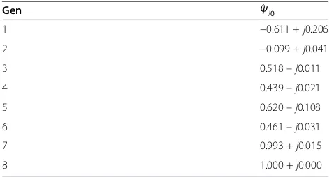
Based on the dominant oscillation mode information above, the eigenvalues of discrete model are calculated. And following the procedure of ARMA-P method shown in Figure 2, the variables vector Ψ^i0 are solved. Using

Gen8 as the reference, the analysis results of Mode I are shown in Table 5.

And the mode shape magnitude and angle are extracted by (14), listed in Table 6.

The ARMA-P method results closely approximate the eigenanalysis results shown in Table 2. The relative errors are mostly no more than 10%, the accuracy of mode shape angle is somewhat better than that of magnitude, and the effectiveness of model order selection is verified again. The mode shape properties can be estimated accurately using the ARMA-P method based on ambient data.

In actual operating condition, noise disturbances such as measurement errors exist continuously in power sys-tems. Since the fluctuation amplitude of ambient signal is relatively small, this type of disturbance cannot be ignored. In order to testify the feasibility of ARMA-P

method in this case, colored noises with certain ampli-tude are added to the original ambient signals. And the identified mode shape results of Mode I from ambient data with 20-dB signal-to-noise ratio (SNR) and 12-dB SNR are indicated in Table 7.

It can be seen from the table that the relative errors of angle results are all less than 11%, which means that the mode shape angle can be identified accurately from am-bient data; the relative errors of magnitude results are a little bigger, yet still less than 15%, which also meets the accuracy requirements of engineering.

Moreover, to test the statistical accuracy of the ARMA-P method, 100 Monte Carlo simulations are run, the mean and root mean square error (RMSE) are calcu-lated. Monte Carlo trials work as to take several inde-pendent measurements on the power system in order to get a sense of the method’s statistical performance. Table 7 Mode shape results of Mode I from ambient signals with different SNR values

SNR (dB) Gen Magnitude (p.u.) Error (%) Angle (rad) Error (%)

20 1 0.647 5.324 3.229 2.318 2 0.135 12.510 3.369 9.523 3 0.530 11.648 5.428 10.970 4 0.458 7.878 −0.044 10.890 5 0.588 1.422 6.282 2.319 6 0.375 11.942 −0.073 8.444 7 0.974 0.851 0.014 10.798 12 1 0.601 12.019 3.169 0.431

2 0.131 8.971 2.783 9.538 3 0.407 14.211 5.468 10.312 4 0.372 12.426 −0.054 9.959 5 0.517 13.430 6.352 3.458 6 0.387 9.045 −0.060 10.424 7 0.861 12.383 0.014 10.364

Table 8 Mode shape with mean and RMSE value of Mode I based on ambient signals

Gen Magnitude (p.u.) Angle (rad)

Mean RMSE Mean RMSE

1 0.717 0.056 3.390 0.051

2 0.109 0.009 3.355 0.055

3 0.517 0.032 5.930 0..070

4 0.440 0.024 −0.048 0.032

5 0.566 0.040 6.177 0.062

6 0.457 0.033 −0.069 0.029

7 0.971 0.010 0.0170 0.031

Table 6 Mode shape results of Mode I in 36-node benchmark system

Gen Magnitude (p.u.) Error (%) Angle (rad) Error (%)

1 0.645 5.564 2.817 10.741

2 0.108 10.000 2.751 10.566

3 0.518 9.283 6.263 2.740

4 0.439 3.294 −0.048 4.000

5 0.629 5.360 6.111 0.472

6 0.462 8.451 −0.066 1.493

7 0.993 1.017 0.015 6.250

Table 5 Results of variables vectorΨ^i0of Mode I

Gen Ψ^i0

1 −0.611 +j0.206

2 −0.099 +j0.041

3 0.518–j0.011

4 0.439–j0.021

5 0.620–j0.108

6 0.461–j0.031

7 0.993 +j0.015

The results of the Monte Carlo trials are listed in Table 8. Obviously, there is a good agreement be-tween the new ARMA-P method and the traditional eigenanalysis. The feasibility of AMRA-P method is further verified.

Actual system example

Now consider the ambient data from China Southern Power Grid as shown in Figure 6. The system contains several interarea modes including two dominant modes, one is the Yunnan-Guizhou mode, about 0.6–0.7 Hz, and another is the Yunnan&Guizhou-Guangdong mode, about 0.4–0.5 Hz. The angle relationship of generators in the Yunnan-Guizhou mode is shown in Figure 7, where the ones on the left are the generators in Yunnan Province, and the ones on the right are the generators in Guizhou Province.

For demonstration purposes, five locations spread across the power grid are selected, including Anshun substation, Gaopo converting plant, and Xingren

converting plant in Guizhou province, and Luoping substation in Yunnan Province, Luodong substation in Guangdong Province.

Ten-minute frequency data were collected from 02:10 to 02:20, on June 14th, 2009. The frequency signal of Luoping substation is shown in Figure 8. Owing to the limitation of phasor measurement, the accuracy of frequency signal shown is limited, and since the power flow was regulated during the data-collecting process, this signal has apparent fluctuations. However, they would not influence the identi-fication of oscillation mode information.

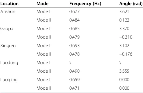
The ARMA-P method is used to identify the mode shape properties from ambient signals. Luoping sub-station was selected as the reference. The analysis results in Table 9 and Figure 9 show the mode shape angle in-formation in China Southern Power Grid.

From Table 9, it can be seen that the system includes two dominant interarea oscillation modes, with the Figure 6Structure diagram of China Southern Power Grid.

Generators in Yunnan Province

Generators in Guizhou Province

Figure 7Angle relationship of generators in Yunnan-Guizhou mode.

0 2 4 6 8 10

49.9 49.92 49.94 49.96 49.98 50 50.02 50.04 50.06 50.08 50.1

Time(min)

F

requency of Luoping substation(Hz)

frequency of mode I at about 0.47 Hz, and the fre-quency of mode II at about 0.68 Hz. Anshun, Gaopo, Xingren, Luoping all participate in the two modes, whereas Luodong only participates in mode I. The plots in Figure 9 indicate that in mode I Anshun, Gaopo, and Xingren swing together against Luoping, which conforms to the angle relationship shown in Figure 7, and in mode II Anshun, Gaopo, Xingren, and Luoping swing together against Luodong. It can be deduced that mode I is the Yunnan-Guizhou mode, and mode II is the Yunnan&Guizhou-Guangdong mode. The analysis results

conform to the mode shape characteristics information that analyzed in advance. The ARMA-P method per-forms well in estimating the mode shape of multiple modes simultaneously based on actual ambient signals in China Southern Power Grid.

Conclusion

A methodology considering the model order selection called ARMA-P, used for estimating the mode shape properties from time-synchronized phasor measure-ments, is presented. Based on its theoretical analysis basis, the approach is applied to a simulation system and measured data from China Southern Power Grid. The results demonstrate that the optimal model order can be selected automatically and efficiently using BIC and the ARMA(2n,2n – 1) modeling procedure. This method works well in estimating the mode shape information of multiple oscillation modes simultaneously based on am-bient signals with different SNR value. And further based on Monte Carlo studies, it is shown that the ARMA-P method can estimate mode shapes with rea-sonably good accuracy.

The algorithm proposed in this article shows great promise for estimating the mode shape properties of power systems. Future work will more rigorously investi-gate its performance including the data length required and the calculation speed.

Table 9 Results of mode shape angle in China Southern Power Grid

Location Mode Frequency (Hz) Angle (rad)

Anshun Mode I 0.677 3.621

Mode II 0.484 0.122

Gaopo Mode I 0.685 3.370

Mode II 0.479 −0.310

Xingren Mode I 0.693 3.102

Mode II 0.478 −0.176

Luodong Mode I \ \

Mode II 0.490 3.555 Luoiping Mode I 0.659 0.000 Mode II 0.471 0.000

30

210

60

240

90

270 120

300 150

330

180 0

30

210

60

240

90

270 120

300 150

330

180 0

(a)

mode I

(b)

mode II

Gaopo Xingren Luoping

Anshun Gaopo Xingren Luodong Luoping

Competing interests

The authors declare that they have no competing interests

Acknowledgment

This study was supported in part by the National Natural Science Foundation of China 51207093 and 51037002, the Natural Science Foundation of Guangdong Province, China S2011040000995, the Foundation for Distinguished Young Talents in Higher Education of Guangdong, China LYM11108, and the Shenzhen Technology Research and Development Foundation JC201105130407A and GJHS20120621154628775.

Author details

1_{College of Mechatronics and Control Engineering, Shenzhen University,}

Shenzhen 518060, China.2_{Department of Electrical Engineering, Tsinghua}

University, Beijing 100084, China.

Received: 29 November 2011 Accepted: 23 December 2012 Published: 26 January 2013

Reference

1. P. Kunder,Power System Stability and Control(McGrawHill, Inc., New York, 1994)

2. J.F. Hauer, C.J. Demeure, L.L. Scharf, Initial results in Prony analysis of power response signals. IEEE Trans. Power Syst.5(1), 80–89 (1990)

3. D.J. Trudnowski, J.W. Pierre,Signal processing methods for estimating small-signal dynamic properties from measured responses, in Analysis of Nonlinear and Non-stationary Inter-area Oscillations: A Time Frequency Perspective

(Springer, New York, 2009)

4. I. Kamwa, G. Trudel, L. Gerin-Lajoie,Low-order black-box models for control system design in large power systems, in IEEE Proceeding of Power Industry

Computer Application Conference(Salt Lake City, 1995), pp. 190–198

5. J.J. Sanchez-Gasca, J.H. Chow, Performance comparison of three

identification methods for the analysis of electromechanical oscillations. IEEE Trans. Power Syst.14(3), 995–1002 (1999)

6. J.W. Pierre, D.J. Trudnowski, M.K. Donnelly, Initial results in electromechanical mode identification from ambient data. IEEE Trans. Power Syst.12(3), 1245–1251 (1997)

7. IEEE Task Force Report,Identification of electromechanical modes in power

systems(The Institute of Electrical and Electronics Engineers, Inc, 2012)

8. L. Vanfretti, L. Dosiek, J.W. Pierre, D.J. Trudnowski, J.H. Chow, R. García-Valle, U. Aliyu, Application of ambient analysis techniques for the estimation of electromechanical oscillations from measured PMU data in four different power systems. Eur. Trans. Electr. Power21(4), 1640–1656 (2011)

9. C. Wu, C. Lu, Y.D. Han, Closed-loop identification of power system based on ambient data. Math. Probl. Eng. (2012). Article ID 632897, 16 (2012) 10. D.J. Trudnowski, Estimating electromechanical mode shape from

synchrophasor measurements. IEEE Trans. Power Syst.23(3), 1188–1195 (2008)

11. G. Liu, V. Venkatasubramanian,Oscillation monitoring from ambient PMU measurements by frequency domain decomposition, in IEEE Proceeding of

Symposium Circuits and Systems(Seattle, 2008), pp. 2821–2824

12. L. Dosiek, D.J. Trudnowski, J.W. Pierre,New algorithm for mode shape estimation using measured data, in IEEE Proceeding of PES General Meeting

(Pittsburgh, 2008), pp. 1–8

13. L. Dosiek, J.W. Pierre, D.J. Trudnowski, N. Zhou,A channel matching approach for estimating mode shape, in IEEE Proceedings of PES General

Meeting(Calgary, 2009), pp. 1–8

14. N. Zhou, Z.Y. Huang, L. Dosiek, D.J. Trudnowski, J.W. Pierre,Electromechanical mode shape estimation based on transfer function identification using PMU

measurements, in IEEE Proceedings of PES General Meeting(Calgary, 2009),

pp. 1–7

15. S. Patrick,Optimization in Signal and Image Processing(Wiley, New Jersey, 2009)

16. H. Akaike,Information theory and an extension of the maximum likelihood principle, in Proceeding of 2nd International Symposium on Information Theory

(Budapest, 1973), pp. 267–281

17. R. Shibata, Selection of the order of an AR model by AIC. Biometrika

63, 117–126 (1976)

18. G. Schwarz, Estimating the dimension of a model. Ann. Stat.6, 461–464 (1978)

19. J. Rissanen, Modeling by shortest data description. Automatica14, 465–471 (1978)

20. M. El, M. Hallin,Order selection, stochastic complexity and Kullback–Leibler information, in Athens Conference on Applied Probability and Time Series

Analysis, vol. II (1995), volume 115 of Lecture Notes in Statist(Springer, New

York, 1996), pp. 291–299

21. J. Rissanen,Stochastic Complexity in Statistical Inquiry(World Scientific, New Jersey, 1989)

22. B.E.P. George, G.M. Jenkins, G.C. Reinsel,Time Series-Forecasting and Controls

(Wiley, New Jersey, 2008)

23. S.M. Pandit, S.M. Wu,Time-Series and System Analysis with Applications

(Krieger Publishing Company, FL, 2006)

24. H. James Douglas,Time Series Analysis(Princeton University Press, Princeton, 1994)

25. A. Blumer, A. Ehrenfeucht, D. Haussler, M. Warmuth, Occam’s Razor. Inf. Process. Lett.24, 377–380 (1987)

doi:10.1186/1687-6180-2013-8

Cite this article as:Wuet al.:New algorithm for mode shape estimation

based on ambient signals considering model order selection.EURASIP

Journal on Advances in Signal Processing20132013:8.

Submit your manuscript to a

journal and benefi t from:

7 Convenient online submission 7 Rigorous peer review

7 Immediate publication on acceptance 7 Open access: articles freely available online 7 High visibility within the fi eld

7 Retaining the copyright to your article