The accuracy of estimation procedures based
on the imputation of plausible values
H. Geerlings
Supervisors:
The accuracy of estimation procedures based
on the imputation of plausible values
H. Geerlings
September 6, 2005
Supervisors: Prof. dr. C.A.W. Glas
ACKNOWLEDGEMENT
I would like to thank Cees Glas and Hans Vos, from the Department of Mea-surement and Data Analysis (MD) at the University of Twente, for their enthousiasm in introducing their field of work to me. They were willing to give me an answer to every question I could come up with during this gradu-ation project. I also greatly appreciate the support I received from my family and friends.
ABSTRACT
In large-scale international educational surveys, such as TIMSS and PISA, data are often collected using complex item administration designs. Usually, Item Response Theory (IRT) models are used to compare the students’ per-formances in such incomplete designs. In many instances, countries want to use the measurements for secondary analyses. One could, for instance, be interested in the relation between achievement in mathematics and predictor variables such as SES or IQ. Some or all variables may be measured using an incomplete design in combination with an IRT model. The most advanced way to analyse these data would be to concurrently estimate the item and person parameters and the regression coefficients using Marginal Maximum Likelihood (MML) or Markov Chain Monte Carlo (MCMC) estimation (see, for instance, Hendrawan, 2004). However, this involves using complex soft-ware in combination with the original responses. An alternative is to use the estimates of the persons latent parameters in a regression analysis. The problem with this approach is that the unreliability of the estimated latent ability parameters must be taken into account. The unreliability has two related sources. The first one is the estimation or standard error; the second one is measurement error. The first one could be typified as random noise. The second one may be typified as bias, for instance, bias caused by the attenuation effect which is the decrease of manifest correlations due to test unreliability (see, for instance, Glas, 1989). To account for these forms of unreliability, practitioners are provided with so-called plausible values, which are random draws from a person’s estimated ability distribution.
distrib-8 Abstract
ution of the multivariate ML estimate or drawing plausible values from this distribution appeared to give the best results. Estimation based on plausible values drawn from the sample distributions of the univariate estimates re-sulted in estimates that displayed the highest attenuation. The method based on computing the expected value of the sample distribution of the multivari-ate posterior estimmultivari-ate and the method drawing plausible values from this distribution resulted in overestimates.
CONTENTS
1. Introduction . . . 11
2. IRT models and estimation procedures . . . 15
2.1 Measurement models . . . 15
2.1.1 Dichotomous models . . . 16
2.1.2 Polytomous models . . . 20
2.2 Estimation procedures . . . 21
2.2.1 Estimation of item parameters . . . 21
2.2.2 Estimation of person parameters and imputation of plausible values . . . 25
3. Simulation study . . . 27
3.1 Data generation . . . 27
3.2 Results . . . 28
4. Application to a real data set . . . 35
4.1 The data set . . . 35
4.2 Results . . . 36
5. Conclusion and discussion . . . 39
5.1 Conclusion . . . 39
5.1.1 Simulation study . . . 39
5.1.2 Application to a real data set . . . 40
5.2 Discussion . . . 40
Appendix 45 A. ML and EAP derivations . . . 47
A.1 ML derivation . . . 47
A.2 EAP derivation . . . 48
1. INTRODUCTION
Classical Test Theory (CTT) has been the main test theory available before the rise of Item Resonse Theory (IRT). The limitations of CTT provided the rationale for developing a new test theory that did not have these dis-advantages. With CTT the item characteristics are population-dependent and person-scores are test-dependent (Hambleton, Swaminathan, & Rogers, 1991). This makes the comparison of test scores of different groups who were administered different tests difficult. Furthermore, it means that a person can have a different estimated true score when making the test as a part of a different group. This is because the estimate of the true score regresses to the mean of the group.
IRT does not have these disadvantages. In IRT, the influence of persons and items on the responses are modelled by different sets of parameters: person and item parameters. The person and item parameters are placed on the same scale, so that direct comparison of person scores is possible. Also, the parameters have the property of invariance: if the model holds, item parameters estimated in one sample are within a linear transformation equivalent to those estimated in a different sample. This means that two tests can be calibrated on the same scale after which the scores of the two tests can be compared. This calibration requires that there is overlap between the tests, for instance, by means of an anchor item design or some persons answering questions of both tests. Another advantage of the property of invariance of IRT is that the trait of an individual is, apart from sampling and measurement error, independent of the group in which the person was measured. The problem mentioned with regard to CTT that one person can score differently on a test when placed in a different group does therefore not occur in an IRT scored test.
12 1. Introduction
uncorrelated with answering any other item correctly, when controlling for item and person parameters (Embretson, & Reise, 2000). However, there do exist IRT models that do not make this assumption (Jannarone, 1986; Verhelst, & Glas, 1993).
In the current research, the measurement precision of eight procedures developed to estimate the item and person parameters of IRT models are investigated. The two most widely used procedures to estimate person pa-rameters are Maximum Likelihood (ML) estimation and Expected A Pos-teriori (EAP) estimation. These two estimation procedures resulted out of respectively a frequentist and a Bayesian approach to estimation. The main difference between these two approaches is that inferences in the latter case are based on the posterior distribution and that the latter makes use of prior distributions. The prior distribution is a beforehand notion about the para-meters, for instance about the mean and variance of the population, often based on some theoretical ground. The posterior distribution incorporates both this prior information and the information from the data. An often noted disadvantage of Bayesian statistics is that the choice of the prior in the parameter estimation procedure is in some way subjective. However, as the sample size increases the weight of the data far outweights that of the prior (Gelman, Carlin, Stern, & Rubin, 1995). Although the forementioned procedures are most widely used and are reported to achieve good results, research has also been directed towards estimation methods that have not yet shown their accuracy but are easier to use in secondary analyses. For exam-ple, a secondary analysis could entail investigating the relationship between two variables, like achievement in mathematics and IQ. Unfortunately, prac-titioners often do not have the software needed to do these analyses with complex methods like MML or MCMC. As an alternative, they are often provided with plausible values. These are values drawn from a distribution describing the estimated ability of a person and the variability around this estimate. Plausible values are used by NAEP (Allen, Carlson, & Zelenak, 1999), PISA (Adams, & Wu, 2002), and TIMSS (Martin, Gregory, & Stem-ler, 2000), among other projects. The aim of this research is to compare the performance of eight estimation procedures and to investigate whether four procedures based on imputation of plausible values can function as reason-able substitutes for using the ML and EAP estimates, taking the uncertainty into account. The investigated procedures and their labels are listed in Table 1.1.
13
Logistic (2PL) model. The results will be described in the next chapter. In this context, an accurate method will be defined as one in which the atten-uation effect does not occur in such a degree that it lowers the estimation of the true correlation. The attenuation effect is caused by the unreliability of tests, and can cause the observed correlation values to be considerably lower than the correlations between the true scores or latent abilities (Scheerens, Glas, & Thomas, 2003). In CTT, corrections for this attenuation have been developed. Spearman’s correction for attenuation (Spearman, 1904) has been employed to estimate a correlation which would be expected if the tests were perfectly reliable. Williams’ general correction for attenuation is similar to Spearman’s, but does not depend upon the assumption that the error scores are uncorrelated with true scores and other sets of error scores (Williams, 1974). It is well known, that applying these corrections using estimates of variance components often leads to correlations above one. In IRT, latent cor-relations can be viewed as corcor-relations corrected for attenuation. Therefore, it is important that an estimation procedure gives results that are relatively unbiased by attenuation. The accuracy of eight estimation procedures is therefore the object of investigation in this study.
The next step has been to apply the procedures that gave the best results in the simulation study to a real data set that has been obtained in a large survey research investigating the health of the Swiss population. The data set consisted of scales with multiple response possibilities and therefore a polytomous IRT-model has been used. The Graded Response Model (GRM; Samejima, 1969) has been used to describe the data. The measurement precision of the procedures under investigation have been compared to that of MCMC estimation and estimation by means of total scores. This report will end with a conclusion and discussion.
Tab. 1.1: Labels and descriptions Label Description
ML U Expected value univariate ML estimate ML M Expected value multivariate ML estimate EAP U Expected value univariate posterior estimate EAP M Expected value multivariate posterior estimate PV ML U Plausible values univariate ML estimate
2. IRT MODELS AND ESTIMATION PROCEDURES
This chapter will start with a description of the most common IRT models for dichotomous and polytomous data. Dichotomous data have two scored re-sponse categories: correct or incorrect, succes or failure, 1 or 0; while polyto-mous data have multiple response categories. In IRT, the probability is mod-elled that a person with a certain ability answers an item correctly, given the item parameters (Hambleton, Swaminathan, & Rogers, 1991). Since these person and item parameters are unknown, they have to be estimated from the data. In this study, both frequentist and Bayesian estimation procedures will be used. The estimation procedures will be described in detail.
2.1 Measurement models
Logistic IRT-models, which model the probability that a person with a cer-tain ability answers an item correctly or answers in a cercer-tain item category, are special cases of the general logistic regression model. Ifxis an observation and λ are parameters then
P(x;λ) = exp (x
Tλ)
1 +exp (xTλ). (2.1)
16 2. IRT models and estimation procedures
parameters. Therefore, the improvement of fit of a more complex model has to be weighted against the fit of the less complex model.
2.1.1 Dichotomous models
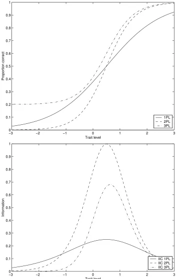
Unidimensional models The 1PL has only one item parameter: the difficulty of the item, β. The two parameter logistic model (2PL) extends this model by adding a discrimination parameter,α, and the 3PL further adds a pseudo-guessing parameter,γ(Hambleton, Swaminathan, & Rogers, 1991). The 3PL is given by
P(Xis = 1|θs, βi, αi, γi) =γi+ (1−γi)
exp[αi(θs−βi)]
1 +exp [αi(θs−βi)]
, (2.2)
in which θs is the ability of person s and βi, αi and γi are the difficulty,
discrimination and pseudo-guessing parameter of item i, respectively. From this formula, the 2PL can be obtained by setting γ to zero and the 1PL by setting α to one. The nominator of the formula denotes the odds of a person s scoring 1 on item i; the denominator adds to this the odds that the same person scores at least 0. The result is the probability of person s scoring 1 rather than 0. It can be seen that when a person has a high ability, for example θ = 1.5, and the difficulty of the item is low, β = −0.5, the difference will be larger than when a person has a lower ability and the item is more difficult. This leads to a formula in which the probability of scoring 1 for this person outweights the probability of scoring 0, leading to a high probability of scoring 1 rather than 0. The pseudo-guessing parameter, γ, results in a probability with a lower asymptote, denoted byγi in (2.2). As an
illustration, the Item Response Curves (IRCs) of the 1PL, 2PL, and 3PL are given in Figure 2.1a, withβ set to 0.5,α to 2.0, andγ to 0.2. IRCs are plots of the Item Response Functions (IRFs), which give the proportion correct score over the ability range, given the item parameters. It can be seen from Figure 2.1a that when the trait level equals the difficulty, the probability of answering an item correctly is 50% for the 1PL and 2PL. This probability is higher for the 3PL, because of the ’guessing’-probability that adds to the 50% chance probability.
2.1. Measurement models 17
−3 −2 −1 0 1 2 3
0 0.1 0.2 0.3 0.4 0.5 0.6 0.7 0.8 0.9 1
Trait level
Proportion correct
1PL 2PL 3PL
−3 −2 −1 0 1 2 3
0 0.1 0.2 0.3 0.4 0.5 0.6 0.7 0.8 0.9 1
Trait level
Information
IIC 1PL IIC 2PL IIC 3PL
18 2. IRT models and estimation procedures
Each of the three logistic models has an equivalent normal ogive version of the model. The normal ogive models (1PNO, 2PNO, and 3PNO) predict very similar probabilities to the 1PL, 2PL and 3PL, respectively (Embretson, & Reise, 2000). Though the latter have more computational simplicity and are more often used than the former, the normal ogive models have the advantage of bearing a relationship to CTT. The 3PNO is given by
P(Xis = 1|θs, βi, αi, γi) =γi+ (1−γi)
Z αi(θs−βi)
−∞
1
(2π)1/2exp(−t
2/2)dt. (2.3)
In this section, until now only the probability of a person answering a single item correctly has been described. Under the assumption of local independence, the probability of a complete response pattern can be com-puted simply by multiplying these probabilities (Mislevy, Johnson, & Muraki, 1992). This point will be returned to later, when discussing the Marginal Maximum Likelihood estimation procedure.
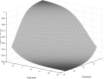
Multidimensional models The singleθ in the formulas described in the pre-vious paragraph signifies that model fit can only be obtained when there is only one dominant underlying latent trait. However, this is not always the case, as with for example mathematics items that also have a reading component that can influence the probability that a person answers the item correctly. In such a case, a multidimensional model will be more appropriate. Also these models are generalizations of the Rasch model. The multidimen-sional versions of the 3PLM and 3PNO are given by
P(Xis = 1|θs, βi, αi, γi) =γi+ (1−γi)
exp (Pmαimθsm+δi)
1 +exp (Pmαimθsm+δi)
, (2.4)
and
P(Xis = 1|θs, βi, αi, γi) =γi+ (1−γi)
Z ∞
−zis
1
(2π)1/2exp(−t
2/2)dt, (2.5)
respectively, in which zis is defined as Pmαimθsm +δi and where δi is the
easiness intercept for itemi. This intercept relates to the item difficulty and discrimination parameter as
βi =
δi
q
1 +Pmαim2
, (2.6)
2.1. Measurement models 19 −4 −2 0 2 4 −3 −2 −1 0 1 2 3 0.2 0.3 0.4 0.5 0.6 0.7 0.8 0.9 1 Trait level Trait level Proportion correct
Fig. 2.2: Item response surface for a multidimensional IRT model
Models incorporating item content factors There have been developed both uni- and multidimensional models that incorporate item content factors into the model. These models are appropriate when there are more than one item content factor defined in the test. A uni- and a multidimensional case of this kind of models are respectively the linear logistic latent trait model (LLTM; Fischer, 1973), given by (2.7), and the general component latent trait model (GLTM; Embretson, & Reise, 2000), given by (2.8). That is,
P(Xis = 1|θs, τk) =
exp (θs−Pkτkqik)
1 +exp(θs−Pkτkqik)
, (2.7)
and
P(Xis = 1|θs, τk) =
Y
m
exp (θsm−Pkτkmqikm)
1 +exp (θsm−Pkτkmqikm)
. (2.8)
In (2.7) and (2.8), qik indicates the value of stimulus factor k in item i and
20 2. IRT models and estimation procedures
2.1.2 Polytomous models
In polytomous models, it is not the probability that a person answers an item correctly that is modelled, but the probability that this person answers in one of the categories indexed j = 1, ..., mi. The generalized partial credit
model (GPCM; Muraki, 1992), like the partial credit model (PCM; Masters, & Wright, 1997), models this probability by means of the item parameter δij that governs the probability of scoring x rather than x-1 on item i. The
resulting model is
Pix(θs) =
exp [Px
j=0αi(θs−δij)]
Pmi
r=0exp[Prj=0αi(θs−δij)]
, (2.9)
withδi0 = 0. From (2.9), the PCM can be obtained by setting αi to one, and
the result will be a generalization of the 1PL as described in the previous section. In that case, the item parameters can be estimated using Conditional Maximum Likelihood (CML). Although the GPCM has desirable properties, caution should be taken when interpreting the item parameters. Becauseδij
is not equivalent to the difficulty parameter of category j alone, but is also related to categoryj-1, this parameter cannot be interpreted as the difficulty parameter in for example the 1PL (Verhelst, Glas, & De Vries, 1997).
The same problem is encountered when using the Graded Response Model (GRM; Samejima, 1969). This model considers the probability of scoring in category j as the difference between the probability of scoring at least in categoryj and the probability of scoring at least in category j+ 1.
In order to overcome this difficulty, Verhelst, Glas, and De Vries (1997) developed the steps model to analyze partial credit. This model assumes that every item consists of several item steps,h= 1, ..., mi, that a person can take
or can stumble upon. These item steps then can be viewed as dichotomous Rasch items. The number of item steps taken within item i can be denoted as
ris = mi
X
h=1
dishyish (2.10)
in whichdishis the indicator variable which takes the value 1 if the item step
was taken by personsand the value 0 if this was not the case. Ifdish = 1,yish
can take the value of 1 if a correct response was given to this item step, and 0 if an incorrect response was given. If the item step was not taken,dish= 0,
yish takes the value of a dummy, an arbitrary constant. The probability of
answering an item in a certain category can then be given by
P(yis|θs, βi) =
exp(risθs−Prhis=1βih)
Qmin(mi,ris+1)
h=1 (1 +exp(θs−βih))
2.2. Estimation procedures 21
This model has the advantage that, in contrast to the PCM, the item pa-rameters can be interpreted as the difficulty of one category, unrelated to other categories. Another advantage is that this model can be estimated us-ing every computer package for dichotomous items that can handle missus-ing data.
In this section only the most widely used IRT models have been described to explain which factors can be included in IRT models. Therefore, it should be noted that there are many more models and generalizations of these mod-els available. For a more extended overview of IRT modmod-els the reader is referred to Embretson and Reise (2000).
2.2 Estimation procedures
Three classes of estimation procedures will be described. The first class en-tails estimation of item parameters using all data, also called the calibration phase of an estimation process. The methods of this class that will be de-scribed here are Marginal Maximum Likelihood (MML) and Markov Chain Monte Carlo (MCMC) estimation. The second class entails estimation of person parameters, and the methods of this class that will be described are Maximum Likelihood (ML) and Expected A Posteriori (EAP) estimation. The methods based on imputation of plausible values form the third class. Although these methods make use of drawings from the ability distributions of persons, these methods can not be used to estimate the abilities of single persons, because of the randomness of the drawings. However, they can be used to compute population statistics. Each of the methods in the second and third class will be discussed in the context of estimating the correlation between two or more variables, for example, the scores on a mathematics and an IQ test. In both a frequentist and a Bayesian framework, it is possible to draw plausible values for each variable seperately and from a combined estimated distribution of the variables.
2.2.1 Estimation of item parameters
Marginal Maximum Likelihood estimation A frequentist approach to
22 2. IRT models and estimation procedures
1−p, over all items:
L(p;x1, x2, ...xk) = k
Y
i=1
pxi(1−p)1−xi. (2.12)
The former probability is then given by one of the probability models as were described in the previous sections. It can be seen from (2.12) that when a person answers an item correctly the part that declares the probability of an incorrect response, 1−p, vanishes from the equation, and similarly that when a person answers an item incorrectly, the probability of a correct response vanishes from the equation. The likelihood function is maximized to obtain that value of p for which the data have the highest likelihood of occuring (Eggen, & Sanders, 1993). It is generally known that one can obtain the maximum of a function by setting the derivative of this function to zero, and this is also how the maximum likelihood functions are derived. To make the derivations easier, the logarithm of the likelihood function is taken to compute the derivative, because this changes a product into a sum and results in the same maximum. Application to the likelihood function gives
lnL(p;x1, x2, ...xk) = k
X
i=1
xilnp+ (1−xi) ln (1−p), (2.13)
and results in the equations
dlnL(p;x1, x2, ...xk)
dp = k X i=1 xi p − 1−xi
1−p = 0. (2.14)
There are three ML-estimators: Joint Maximum Likelihood (JML), Con-ditional Maximum Likelihood (CML), and Marginal Maximum Likelihood (MML) estimation. JML estimates the person and item parameters simulta-neously through an iterative process in which each time the parameters are improved in order to approach the final solution closer each time (Eggen, & Sanders, 1993). There are two problems with this approach. First, it is impossible to obtain parameter estimates when a person scores in an ex-treme way; that is, when a person answers all questions right or all questions wrong. Secondly, the estimators of the item parameters are inconsistent. A consistent estimator improves the accuracy of the estimation of the parame-ters, by means of augmenting the information on the parameter through a larger sample. The problem here is that with every new person a new ability parameter has to be estimated, and that the number of parameters that have to be estimated grows as fast as the sample size does.
2.2. Estimation procedures 23
that for the 1PL, when computing the probability of a certain response pat-tern, and conditioning on the score groups denoted byθ, theθ’s are removed from the equation. This has the advantage that this estimator is independent on the population sample. A different sample of the same size can though provide a different estimation precision (Eggen, & Sanders, 1993). After having estimated the item parameters, the person parameters can be easily obtained by imputing the item parameters in the IRT-model.
A different way of removing the person parameters from the likelihood is provided by MML estimation. MML assumes the θ’s to be from a certain distribution, for example the normal distribution. The conditional probabil-ities of a certain response pattern x can be obtained by multiplying these probabilities with the probability that a certain θ occurs, and adding these probabilities. When there areW different values that θ can take, this can be described as
P(x, θj) = W
X
j=1
P(x|θj)P(θj). (2.15)
By making this function continuous overθ, so with an infinitely large number W, the problem of solving this equation becomes easier. The function can be made continuous by, for example, assuming that the values of θ come from the normal distribution, which will be denoted here asg(θ). The probability of a certain response pattern then becomes
P(x) = Z +∞
−∞ P(x|θ)g(θ)dθ (2.16)
It can be seen thatP(x) is no longer dependent on θ, having been integrated out, but on the item parameters and the mean and standard deviation of the normal distribution. Taking the product over the values of (2.16) for all observed response patterns and taking the logarithm of this leads to a mar-ginal likelihood and the MML estimator. Although MML is computationally heavy due to the integral, it produces consistent parameter estimates. This means that the estimates approach the true parameters asymptotically. A disadvantage of this method is that when the assumption of a certain distri-bution of the person parameters is not correct, errors in the item parameter estimates can occur.
Markov Chain Monte Carlo estimation A different approach to
24 2. IRT models and estimation procedures
model in the parameter vector φ to account for the uncertainty that ac-companies the estimation (Gelman, Carlin, Stern, & Rubin, 1995). A prior distribution for φ is furthermore defined, unconditional on the data, as a prediction of howφ is distributed. As a prior distribution forθ, for example, it can be assumed that θ is normally distributed with µ= 0 and σ = 1. To find a posterior distribution for the parameter that describes the data, x,
data augmentation is used. In this process, latent parameters Z are added to the model. Z consists of draws from the normal distribution according to the response pattern, x. If x= 1, a draw is taken from the left part of zero in N(µ,1). Similarly, if x = 0, a draw is taken from the right part of zero. The new parameter Z is added to φ.
The prior distribution is combined with the information provided by the data by means of Bayes’ rule to obtain the posterior distribution (Gelman, Carlin, Stern, & Rubin, 1995). This can be written as
P(φ|y) = P(φ)P(x|φ)
P(x) . (2.17)
In this equation the likelihood of the data, given a certain φ is multiplied with the prior, and the result is divided by the marginal likelihood. It can be seen that when the sample size increases the influence of the prior decreases. Since in many cases it is not feasible to perform calculations on the pos-terior distribution directly, inferences are made through simulation from this distribution (Gelman, Carlin, Stern, & Rubin, 1995). In the second study, described in chapter four, one particular MCMC method has been used to estimate the correlations between variables: the Gibbs sampler. The Gibbs sampler starts with initial guesses at the parameter values of the posterior distribution. Then a cycle of sampling begins, in which each iteration con-sists of a few steps in which one of the parameters is being sampled from the posterior distribution conditional on the other parameters (Albert, 1992). Applied to an IRT model with parameters φ = (θ, β, µ, σ,Z), the algorithm becomes:
Step 1: P(θ|β, µ, σ,Z,Y) Step 2: P(β|θ, µ, σ,Z,Y) Step 3: P(µ, σ|β, θ,Z,Y) Step 4: P(Z|β, θ, µ, σ,Y)
2.2. Estimation procedures 25
2.2.2 Estimation of person parameters and imputation of plausible values
There are several ways to estimate the person parameters when the item parameters of an IRT model have already been estimated. In this study, the correlation between two variables has been computed by taking the expected values of the univariate and multivariate ML and posterior estimates. The first two are based on the ML estimates of θ and their standard errors, the second are based on the posterior expectation and posterior variance of θ. So, in total, four methods have been used that are based on computing the expected value of a certain estimate. The first two, ML U and ML M, use the univariate and multivariate ML estimates, respectively. The derivation of the multivariate ML estimates can be found in Appendix A. The univariate ML estimate is a special case of this estimate and can be obtained by inserting only one variable in the equation. The second two procedures, EAP U and EAP M, use the univariate and multivariate posterior estimates, as given by equations (2.17) and (A.6), respectively. For the computation of the variance of the estimates, we used
V ar(θ) =E(V ar(θ|x)) +V ar(E(θ|x)), (2.18) where E(V ar(θ|x)) is the expected measurement error, or within persons variance, and V ar(E(θ|x)) is the between persons variance (see, Scheerens, Glas, & Thomas, 2003).
Four other procedures have been used in this study, using the same esti-mates. Instead of computing the expected values, plausible values were drawn from these estimated distributions. Plausible values are random draws from a person’s estimated distribution, h(θ|x). Usually five draws are taken from the posterior distribution for each person to account for the uncertainty of the estimates. These values can not be used to estimate a single person’s ability, since in that case an estimation based on only five values would give unreliable results. However, the values can be used to estimate population characteristics. To this end, the weighted mean and the variance of each of the five vectors of plausible values is computed. Additionally, the vari-ance among the five weighted means can be computed and added to the average sampling variance of the vectors. However, this last step is omitted in the practice of NAEP, because of the excessive computation that would be required. Therefore, only the average sampling variance of the first set of plausible values is used in NAEP analyses (Mislevy, Johnson, & Muraki, 1992).
26 2. IRT models and estimation procedures
the plausible values from the multivariate ML or posterior estimates, in which the correlation between the variables is already taken into consideration. This can be seen as estimating the parameters of one single test with multiple dimensions, instead of estimating the parameters of several tests, with each one measuring a different dimension.
In a frequentist framework, the plausible values method (PV ML U) im-plies draws from a normal distribution with µ = ˆθ and σ2(ˆθ) estimated by means of ML. To compute the correlation between two or more variables, separate draws for each variable are needed. The second plausible values method (PV ML M) draws the plausible values from the sample distribution of the multivariate estimate. With m= 1, ..., u dimensions, the likelihood of this distribution can be written as
L(θ1, ..., θu) = u
Y
m=1 [
KYm
i=1
Pi(θm)xim(1−Pi(θm))1−xim]N(θ1, ..., θu|Σ). (2.19)
Taking the logarithm and the derivative over θ of this likelihood results in the multivariate ML estimate,
dlogL dθ =
"
−s1+PKi=1mP(θs1)
−s2+PKm
i=1P(θs2)
#
−Σ−1θ. (2.20)
of which the complete derivation can be found in Appendix A. This is a case of a so called shrinkage estimator, meaning that shrinkage occurs towards the mean of the normal distribution.
The following two plausible values methods are used in a Bayesian frame-work. The first, PV EAP U, draws values from a person’s univariate posterior estimate, as was given in (2.17). The second, PV EAP M, draws values from a person’s multivariate posterior estimate, which can be given by
P(θ1, ..., θm|x,Σθ) = T
Y
t=1
P(xt|θt)N(θ1, ..., θm|Σ), (2.21)
where xt and θt are the response pattern and ability of a person on test t,
3. SIMULATION STUDY
The aim of this simulation study was to investigate the accuracy of several estimation methods based on imputation of plausible values as a substitute for more statistically grounded methods, like the ML estimation method. The accuracy of these methods was measured by the amount of attenuation in the observed correlation between two variables, relative to the true correlation. Since the effect of attenuation also depends on the test length and the sample size, multiple values for these variables were used. The 1PL and 2PL models were used to generate the data and the item parameters were randomly drawn. The difficulty parameters were drawn from the standard normal distribution, and the discrimination parameters were drawn from the uniform distribution on (0.5,1.5).
3.1 Data generation
A program has been made using the Fortran language to retrieve the corre-lation of two variables of which the true correcorre-lation was known in advance. These matrices were estimated in the program by means of the total scores, ML, EAP, and four methods based on imputation of plausible values in a fre-quentist and Bayesian framework. In each framework, plausible values were drawn from univariate and multivariate estimates. A discrepancy between the true correlation and the correlation estimated by any of these methods was interpreted as bias caused by the attenuation effect.
28 3. Simulation study
were drawn in a frequentists framework. The other four vectors of plausible values were randomly drawn in a Bayesian framework: from the univariate and multivariate posterior estimates, respectively. Also, the expected values of both the frequentist and Bayesian uni- and multivariate estimates were computed. The mean was taken of each of these vector valued θ’s, and used to compute the correlations. Similarly, the true correlation and the correlation between the total scores were computed.
Two different sample sizes were used, N = 200,and 1000; three different test lengths, K = 10,20, and 40; and four different correlation values, ρ = .2, .4, .6 and .8; yielding a two-by-three-by-four crossed design. With eight estimation procedures and the computation of the true correlations and the correlations by means of total scores, this lead to 240 correlations. Each of these correlations was replicated 100 times and the mean of these replications was taken to obtain the final 240 correlations. This procedure has been followed for both the 1PL and 2PL model.
3.2 Results
The differences between the correlations as defined beforehand and the esti-mated correlations for the 1PL model are shown in Table 3.1. For the 2PL model, these correlations are given by Table 3.2. The correlation as was read in by the program is given by ρ. Due to random drawing of the values for θ the true correlation computed with these values shows a small difference with ρ.
3.2. Results 29
Tab. 3.1: Difference between θand ˆθ (1PL)
N = 200 N = 1000
ρ K = 10 K = 20 K = 40 K = 10 K = 20 K = 40 True correlation .2 0.0048 0.0028 0.0045 0.0021 0.0016 0.0008 Total scores 0.0786 0.0418 0.0280 0.0752 0.0454 0.0246
ML U 0.1347 0.1118 0.0949 0.1343 0.1134 0.0919
ML M 0.0098 0.0020 0.0038 0.0064 0.0042 0.0008
EAP U 0.1023 0.0520 0.0298 0.0979 0.0517 0.0261
EAP M -0.0258 -0.0372 -0.0293 -0.0303 -0.0342 -0.0304
PV ML U 0.1052 0.0762 0.0488 0.1104 0.0753 0.0444
PV ML M -0.0035 -0.0026 -0.0013 0.0069 -0.0032 0.0032
PV EAP U 0.1295 0.0796 0.0543 0.1230 0.0864 0.0486
PV EAP M -0.0267 -0.0401 -0.0309 -0.0290 -0.0318 -0.0300 True correlation .4 0.0018 -0.0069 -0.0034 0.0018 -0.0026 0.0001 Total scores 0.1500 0.0807 0.0511 0.1444 0.0836 0.0499
ML U 0.2672 0.2199 0.1876 0.2647 0.2222 0.1855
ML M 0.0113 0.0020 0.0040 0.0094 0.0032 0.0020
EAP U 0.2036 0.0981 0.0540 0.1983 0.1028 0.0527
EAP M -0.0517 -0.0651 -0.0531 -0.0532 -0.0640 -0.0556
PV ML U 0.2137 0.1322 0.0884 0.2132 0.1413 0.0884
PV ML M 0.0068 0.0085 0.0087 0.0068 0.0063 0.0036
PV EAP U 0.2477 0.1569 0.0982 0.2451 0.1657 0.0997
PV EAP M -0.0552 -0.0640 -0.0514 -0.0533 -0.0648 -0.0531 True correlation .6 -0.0070 0.0031 0.0092 0.0017 0.0012 0.0026 Total scores 0.2135 0.1357 0.0851 0.2111 0.1347 0.0772
ML U 0.3962 0.3401 0.2853 0.3942 0.3382 0.2801
ML M 0.0100 0.0084 0.0109 0.0124 0.0083 0.0053
EAP U 0.2863 0.1575 0.0903 0.2828 0.1753 0.0818
EAP M -0.0579 -0.0694 -0.0605 -0.0583 -0.0709 -0.0660
PV ML U 0.3177 0.2233 0.1383 0.3156 0.2189 0.1340
PV ML M 0.0092 0.0178 0.0054 0.0134 0.0091 0.0031
PV EAP U 0.3598 0.2576 0.1541 0.3631 0.2524 0.1476
PV EAP M -0.0603 -0.0723 -0.0622 -0.0588 -0.0699 -0.0666 True correlation .8 -0.0010 -0.0023 -0.0022 -0.0014 0.0009 -0.0002 Total scores 0.2823 0.1737 0.0982 0.2781 0.1703 0.0961
ML U 0.5239 0.4492 0.3708 0.5231 0.4456 0.3706
ML M 0.0083 0.0065 0.0030 0.0079 0.0064 0.0027
EAP U 0.3763 0.2006 0.1048 0.3702 0.1975 0.1032
EAP M -0.0423 -0.0529 -0.0566 -0.0419 -0.0536 -0.0561
PV ML U 0.4246 0.2812 0.1738 0.4201 0.2829 0.1749
PV ML M 0.0114 0.0121 0.0038 0.0092 0.0050 0.0005
PV EAP U 0.4760 0.3320 0.1972 0.4814 0.3286 0.1954
30 3. Simulation study
Tab. 3.2: Difference between θand ˆθ (2PL)
N = 200 N = 1000
ρ K = 10 K = 20 K = 40 K = 10 K = 20 K = 40 True correlation .2 -0.0008 0.0050 0.0017 -0.0081 0.0004 -0.0045 Total scores 0.0679 0.0474 0.0301 0.0675 0.0434 0.0200
ML U 0.1278 0.1116 0.0963 0.1271 0.1100 0.0883
ML M 0.0083 0.0068 0.0049 0.0072 0.0061 -0.0026
EAP U 0.0850 0.0540 0.0330 0.0801 0.0479 0.0215
EAP M -0.0285 -0.0307 -0.0274 -0.0307 -0.0320 -0.0326
PV ML U 0.1012 0.0724 0.0450 0.0964 0.0713 0.0385
PV ML M 0.0075 0.0035 -0.0085 0.0034 0.0058 0.0018
PV EAP U 0.1243 0.0802 0.0565 0.1216 0.0845 0.0450
PV EAP M -0.0263 -0.0256 -0.0262 -0.0305 -0.0321 -0.0308 True correlation .4 -0.0106 0.0069 -0.0024 0.0012 0.0021 -0.0005 Total scores 0.1457 0.0890 0.0493 0.1505 0.0921 0.0497
ML U 0.2642 0.2254 0.1863 0.2673 0.2245 0.1839
ML M 0.0059 0.0059 0.0003 0.0104 0.0107 0.0012
EAP U 0.1922 0.0980 0.0638 0.1787 0.1039 0.0546
EAP M -0.0534 -0.0633 -0.0547 -0.0504 -0.0569 -0.0549
PV ML U 0.2189 0.1495 0.0868 0.2229 0.1463 0.0871
PV ML M 0.0153 -0.0003 -0.0041 0.0084 0.0062 0.0085
PV EAP U 0.2624 0.1723 0.1116 0.2643 0.1750 0.1011
PV EAP M -0.0548 -0.0650 -0.0544 -0.0454 -0.0530 -0.0560 True correlation .6 0.0114 -0.0052 0.0080 -0.0020 -0.0007 0.0006 Total scores 0.2356 0.1284 0.0773 0.2103 0.1250 0.0756
ML U 0.3997 0.3348 0.2772 0.3893 0.3299 0.2792
ML M 0.0199 0.0055 0.0092 0.0119 0.0065 0.0032
EAP U 0.2857 0.1429 0.0813 0.2510 0.1479 0.0837
EAP M -0.0532 -0.0730 -0.0606 -0.0591 -0.0722 -0.0672
PV ML U 0.3412 0.2095 0.1367 0.3102 0.2112 0.1364
PV ML M 0.0155 0.0069 0.0094 0.0143 0.0061 0.0008
PV EAP U 0.3975 0.2556 0.1572 0.3828 0.2624 0.1585
PV EAP M -0.0522 -0.0736 -0.0585 -0.0575 -0.0719 -0.0664 True correlation .8 0.0028 0.0007 0.0010 0.0003 0.0025 0.0003 Total scores 0.2895 0.1858 0.0956 0.2636 0.1690 0.0943
ML U 0.5238 0.4526 0.3671 0.5053 0.4422 0.3662
ML M 0.0118 0.0064 0.0056 0.0107 0.0077 0.0025
EAP U 0.3437 0.2019 0.1045 0.3207 0.1946 0.1057
EAP M -0.0383 -0.0534 -0.0532 -0.0423 -0.0526 -0.0559
PV ML U 0.4328 0.2965 0.1688 0.3982 0.2839 0.1717
PV ML M 0.0063 0.0088 0.0073 0.0115 0.0037 0.0042
PV EAP U 0.5225 0.3601 0.1932 0.4846 0.3466 0.2046
3.2. Results 31
0.2 0.3 0.4 0.5 0.6 0.7 0.8
−0.05 0 0.05 0.1 0.15 0.2 0.25 0.3 0.35 0.4 0.45 Rho
Difference from rho
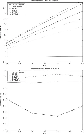
Unidimensional methods − 10 items
True correlation Total scores ML U EAP U PV ML U PV EAP U
0.2 0.3 0.4 0.5 0.6 0.7 0.8
−0.08 −0.07 −0.06 −0.05 −0.04 −0.03 −0.02 −0.01 0 0.01 0.02 Rho
Difference from rho
Multidimensional methods − 10 items
True correlation ML M EAP M PV ML M PV EAP M
32 3. Simulation study
0.2 0.3 0.4 0.5 0.6 0.7 0.8
−0.05 0 0.05 0.1 0.15 0.2 0.25 0.3 0.35 0.4 0.45 Rho
Difference from rho
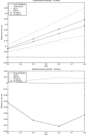
Unidimensional methods − 20 items
True correlation Total scores ML U EAP U PV ML U PV EAP U
0.2 0.3 0.4 0.5 0.6 0.7 0.8
−0.08 −0.07 −0.06 −0.05 −0.04 −0.03 −0.02 −0.01 0 0.01 0.02 Rho
Difference from rho
Multidimensional methods − 20 items
True correlation ML M EAP M PV ML M PV EAP M
3.2. Results 33
0.2 0.3 0.4 0.5 0.6 0.7 0.8
−0.05 0 0.05 0.1 0.15 0.2 0.25 0.3 0.35 0.4 0.45 Rho
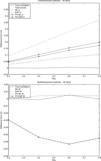
Difference from rho
Unidimensional methods − 40 items
True correlation Total scores ML U EAP U PV ML U PV EAP U
0.2 0.3 0.4 0.5 0.6 0.7 0.8
−0.08 −0.07 −0.06 −0.05 −0.04 −0.03 −0.02 −0.01 0 0.01 0.02 Rho
Difference from rho
Multidimensional methods − 40 items
True correlation ML M EAP M PV ML M PV EAP M
34 3. Simulation study
ρ =.6 and decrease again in attenuation at ρ =.8. The methods using the multivariate ML estimate, ML M and PV ML M, also lie close in their mean difference fromρ. Furthermore, they both are closest to the true correlation. This can also be read from Table 3.3. These methods have a mean deviation fromρ of less than .0100 and with an increasing number of items in the tests the estimated correlations closely approach the true correlation. Closest to the true correlations after ML M and PV ML M are the multivariate EAP estimates and the plausible values from the multivariate posterior estimates. However, these methods give overestimates of the correlation.
Tab. 3.3: Mean deviation and standard error correlations
Min. Max. Mean S.D.
True correlation -0.0106 0.0114 0.0005 0.0042 Total scores 0.0200 0.2895 0.1169 0.0737
ML U 0.0883 0.5239 0.2797 0.1328
ML M -0.0026 0.0199 0.0066 0.0040
EAP U 0.0215 0.3763 0.1411 0.0955
4. APPLICATION TO A REAL DATA SET
To investigate the generalizability of the results of the previous chapter, the estimation methods that appeared to give the best results, ML M and PV ML M, have been applied to a real data set. The correlations were computed with different scales of the data set as variables. Again, the results were interpreted by the degree in which attenuation was present. Correlations computed by means of MCMC and by means of the total scores were used as a reference. MCMC gives results without much attenuation, and the correlations resulting from this method could therefore be used as a comparison. The correlations obtained by means of the total scores were considered as a baseline for the attenuation effect.
4.1 The data set
The data has been provided by the Institute for Evaluative Research in Or-thopaedics from the University of Bern. A large survey research has been conducted among the Swiss population by means of one questionnaire trans-lated in German and French; the two main languages of Switzerland. In this research, the data obtained from the German questionnaire has been used. Respectively 17.486 persons filled in this questionnaire. Of these, 7104 were filled in by men, 9942 by women and 440 by people who did not enter their gender. The respondents were aged between 17 and 98 years old, with a mean of 49 years old.
36 4. Application to a real data set
(Skills), and walking for 30 minutes (Walking). The scales consisted of re-spectively 9, 9, 9, 15, 8, 7, and 7 items. The questions were constructed on a seven-point scale, from ’No difficulties’ to ’Not longer possible’. The tables in Appendix B show for each item in each scale the number of valid cases, the number of missing cases, the mean response, and the mean response subdivided by gender. The scales have been grouped in three to result in three tests of three variables. The MCMC and total scores matrices have been computed with RSP and SPSS, respectively, using all data. The two multivariate ML methods have been computed with the same program that was used in the simulation study, but because the items were polytomous, the GRM (Samejima, 1969) was used instead of the 1PL and 2PL models. A random draw of 2000 respondents has been taken from the complete sample to reduce the sample size.
4.2 Results
Tables 4.1, 4.2, and 4.3 give the covariance and correlation matrices com-puted with MCMC, total scores, ML M, and PV ML M, respectively. All three tables show that ML M and PV ML M give results closer to the true correlation than the correlations computed by means of the total scores, as was also shown by the simulation study. Furthermore, from these tables it can be seen that PV ML M performs even slightly better than ML M.
4.2. Results 37
Tab. 4.2: Covariances and correlations Agility-Difficulty-Force Covariances Correlations Agili Diffi Force Agili Diffi Force MCMC Agili 1.689 1.043 1.177 1.000 0.655 0.634 Diffi 1.043 1.504 1.167 0.655 1.000 0.666 Force 1.177 1.167 2.041 0.634 0.666 1.000 Total scores Agili 0.644 0.218 0.642 1.000 0.550 0.592 Diffi 0.218 0.305 0.325 0.550 1.000 0.585 Force 0.642 0.325 1.441 0.592 0.585 1.000 ML M Agili 1.621 0.899 0.956 1.000 0.582 0.546 Diffi 0.899 1.472 1.020 0.582 1.000 0.612 Force 0.956 1.020 1.889 0.546 0.612 1.000 PV ML M Agili 1.490 0.834 0.968 1.000 0.615 0.601 Diffi 0.834 1.233 0.938 0.615 1.000 0.641 Force 0.968 0.938 1.740 0.601 0.641 1.000
38 4. Application to a real data set
5. CONCLUSION AND DISCUSSION
In this section the conclusions drawn from the results of the simulation study and the real data application will be described. Also, the relevance of the results for the practice of data analysis will be described. In the discussion, this research will be reviewed and limitations in generalization of the results will be considered.
5.1 Conclusion
The first part of this research consisted of a literature study, of which the focus was on several often used estimation procedures. Marginal Maximum Likelihood (MML) and Markov Chain Monte Carlo (MCMC) estimation have both proved their accuracy in past research (Kim, 2001; Wollack, Bolt, Co-hen, & Lee, 2002). However, they also have disadvantages. Both procedures are relatively complex in their computations and can not be done when only statistical packages like SPSS and SAS are available. When proving accurate enough, plausible values drawn out of the ML or posterior estimates could provide a solution to this problem. These are values that can be considered as single data points and can be used to compute mean population statistics. It should be noted that plausible values can not be used to compute person statistics, because of the randomness of the drawings.
5.1.1 Simulation study
40 5. Conclusion and discussion
methods displayed the least influence by the number of items in the tests, and gave the most stable results.
The methods based on imputation of plausible values drawn from uni-variate and posterior estimates did not perform as well. They resulted in computed correlations with a considerable attenuation effect. The methods using the posterior estimates, resulted in estimated correlations that were overestimates of the true correlation. The size of the deviations from the true correlations was such, that application in secondary analyses of plausi-ble values drawn from posterior estimates is dissuaded.
5.1.2 Application to a real data set
Because the data in the simulation study were randomly generated and not obtained by a real data set, the second part of the research focussed on the generalizability of the results through an application of PV ML M and ML M to a data set obtained by a health survey. The correlations estimated by means of these methods were compared to the correlations obtained by means of MCMC and the total scores. Seven scales out of this data set were used and grouped by three to result in three tests of three variables. Also in this study, the two methods using the multivariate ML estimate appeared to function reasonably well. They both gave correlations higher than the correlations computed by means of the total scores and correlations closer to the MCMC correlations. Drawing plausible values from the multivariate ML estimates seemed to function even slightly better than computing the expected values of these estimates.
5.2 Discussion
5.2. Discussion 41
BIBLIOGRAPHY
[1] Adams, R., & Wu, M. (2002).Pisa 2000 technical report.Paris, OECD.
[2] Albert, J.H. (1992). Bayesian estimation of normal ogive item response functions using Gibbs sampling. Journal of Educational Statistics, 17,
251-269.
[3] Allen, N.L.,Carlson, J.E., & Zelenak, C.A. (1999). The NAEP 1996 Technical Report. USA: Education Publications Center.
[4] Eggen, T.J.H.M., & Sanders, P.F. (Eds.) (1993). Psychometrie in de praktijk.Arnhem: Cito.
[5] Embretson, S. E. & Reise, S. P. (2000). Item response theory for psy-chologists.Mahwah, NJ: Lawrence Erlbaum.
[6] Fischer, G.H. (1973). The linear logistic model as an instrument in educational research. Acta Psychologica, 37, 359-374.
[7] Gelman, A, Carlin, J.B., Stern, H.S., & Rubin, D.B. (1995).Bayesian Data Analysis. London: Chapman and Hall.
[8] Glas, C.A.W. (1989). Contributions to estimating and testing Rasch models. Arnhem: Cito.
[9] Hambleton, R.K., Swaminathan, H., & Rogers, H.J. (1991). Funda-mentals of item response theory.Newbury Park, CA: Sage.
[10] Hendrawan, I. (1991).Statistical tests of item response models: power and robustness.Enschede, NL: University of Twente.
[11] Jannarone, R. J. (1986). Conjunctive item response theory kernels.
Psychometrika, 51, 357-373.
[12] Kim, S.H. (2001). An evaluation of a Markov Chain Monte Carlo method for the Rasch model. Applied Psychological Measurement, 25,
44 Bibliography
[13] Martin, M.O., Gregory, K.D., & Stemler, S.E. (Eds.) (2000). TIMSS 1999 Technical Report. USA: Boston College.
[14] Masters, G.N., & Wright, B.D. (1997). The partial credit model. In Van der Linden, W.J., & Hambleton, R.K. (1997).Handbook of modern item response theory. New York: Springer.
[15] Mislevy, R.J., Johnson, E.G., & Muraki, E. (1992). Scaling procedures in NAEP.Journal of Educational Statistics, 17, 131-154.
[16] Muraki, E. (1992). A generalized partial credit model: application of an EM algorithm. Applied Psychological Measurement, 16,159-176.
[17] Rasch, G. (1960).Probabilistic models for some intelligence and attain-ment tests. Copenhagen: Danish Institute for Educational Research.
[18] Samejima, F. (1969). Estimation of latent ability using a pattern of graded scores. Psychometrika, Monograph Supplement, No. 17.
[19] Scheerens, J., Glas, C.A.W., & Thomas, S.M. (2003).Educational Eval-uation, Assessment, and Monitoring. Swets and Zeitlinger.
[20] Spearman, C. (1904). The proof and measurement of association be-tween two things.American Journal of Psychology, 15, 72-101.
[21] Steward, G.W. (2000). The decompositional approach to matrix com-putation. Computing in Science & Engineering, 2, 50-59.
[22] Verhelst, N.D., & Glas, C.A.W. (1993). A dynamic generalization of the Rasch model.Psychometrika, 58, 395-415.
[23] Verhelst, N.D., Glas, C.A.W., & De Vries, H.H. (1997). A steps model to analyze partial credit. In W.J.van der Linden and R.K.Hambleton (Eds.), Handbook of modern item response theory. (pp.123-138). New York, NJ: Springer.
[24] Williams, R.H. (1974). The effect of correlated errors of measurement on correlations among tests: a correlation for Spearman’s correction for attenuation.The Journal of Experimental Education, 43, 63-65.
A. ML AND EAP DERIVATIONS
A.1 ML derivation
The likelihood of m = 1, ..., u ability values on m = 1, ..., u specific tests, given the data, can be given by
L(θ1, ..., θu) = u
Y
m=1 [
KYm
i=1
Pi(θm)xim(1−Pi(θm))1−xim]N(θ1, ..., θu|Σ), (A.1)
in which Pi is an IRT model and N(θ1, ..., θu|Σ) is the multivariate normal
distribution of the u variables:
N(θ1, ..., θu|Σ) =
1
(2π)n/2q|Σ|exp(− 1 2θ
tΣ−1θ). (A.2)
In this example the 1PL will be used. With the assumption that the mean of the population is zero, the logarithm of this function becomes
logL(θ) = log
u X m=1 [ Km X i=1
Pi(θm)xim(1−Pi(θm))1−xim]+logN(θ1, ..., θu|Σ). (A.3)
Simplifying the equation and inserting the IRT model forPi gives
logL(θ) =Pum=1PiK=1mxim(Pum=1θsm+δi)−log(1 +exp(Pmu=1θsm+δi))−
log(2π)n/2q|Σ| − 1 2θ
tΣ−1θ.
(A.4) Taking the derivative overθ of this loglikelihood results in the ML estimate. Letsm be defined asPKi=1mxim, so it is the total score on variablem. Written
in matrix form, and with two variables, it can be seen that the ML esti-mate reduces to the two single ability estiesti-mates minus the derivative of the logarithm of the normal distribution,
dlogL dθ =
"
−s1 +PKm
i=1P(θs1) −s2 +PKm
i=1P(θs2)
#
48 A. ML and EAP derivations
A.2 EAP derivation
The expected value of the multivariate posterior estimate forθm can be given
by
E(θm) =
Z +∞
−∞ θmP(θ|x)dθ1, ..., dθm, (A.6)
in which θm is the m’th element of the vector E(θ|x). Like the estimated
univariate posterior distribution, this distribution is a combination of the prior and the information provided by the data:
E(θm) =
Z +∞
−∞ θm
Qu
m=1P(xm|θm)g(θ1, ..., θu)dθm
R+∞ −∞
Qu
m=1P(xm|θm)g(θ1, ..., θu)dθm
B. SCALE STATISTICS
Tab. B.1: Mean, standard error and reliability of the scales
Scale Mean SE α
Difficulty 5.65 22.508 .850 Mobility 5.64 27.106 .936 Skills 5.29 34.652 .782 Agility 5.03 104.041 .849 Force 4.76 56.620 .858 Walking 5.46 28.486 .891 Activity 5.36 28.364 .859
Tab. B.2: Scale statistics
Scale N valid N missing Mean Mean males Mean females
Difficulty 01 16452 1034 5.69 5.73 5.67
02 16422 1064 5.70 5.75 5.67
03 16408 1078 5.70 5.74 5.68
04 16545 941 5.33 5.44 5.26
05 16340 1146 5.70 5.74 5.68
06 16308 1178 5.59 5.59 5.59
07 16395 1091 5.57 5.67 5.50
08 16353 1133 5.81 5.80 5.82
09 14695 2791 5.78 5.74 5.82
50 B. Scale statistics
Scale N valid N missing Mean Mean males Mean females
Mobility 01 16746 740 5.84 5.86 5.83
02 16763 723 5.48 5.56 5.43
03 16762 724 5.60 5.66 5.57
04 16708 778 5.61 5.66 5.59
05 16695 791 5.70 5.77 5.65
06 16752 734 5.67 5.70 5.65
07 16688 798 5.82 5.86 5.80
08 16672 814 5.68 5.73 5.66
09 16713 773 5.38 5.46 5.33
Skills 01 17030 456 5.94 5.94 5.94
02 16946 540 5.52 5.53 5.51
03 17001 485 5.95 5.97 5.94
04 16996 490 5.76 5.93 5.65
05 16953 533 5.81 5.91 5.75
06 16941 545 5.58 5.68 5.53
07 16871 615 5.37 5.48 5.30
08 16602 884 4.72 4.96 4.55
09 16366 1120 2.97 3.39 2.67
Agility 01 17117 369 5.80 5.80 5.81
02 17100 386 5.84 5.84 5.85
03 17088 398 5.61 5.66 5.58
04 17039 447 5.73 5.75 5.72
05 17100 386 5.90 5.90 5.90
06 17106 380 5.94 5.93 5.94
07 17100 386 5.94 5.95 5.94
08 17083 403 5.91 5.92 5.91
09 17035 451 5.81 5.82 5.81
10 16970 516 5.49 5.46 5.52
11 17038 448 5.41 5.43 5.40
12 16999 487 4.33 4.01 4.57
13 16965 521 3.34 2.87 3.67
14 16975 511 2.50 2.14 2.76
15 16832 654 1.86 1.93 1.82
Force 01 17092 394 5.95 5.97 5.94
02 17070 416 5.58 5.67 5.53
03 17002 484 5.14 5.40 4.97
04 17059 427 5.66 5.81 5.56
05 17070 416 5.05 5.59 4.69
06 17026 460 4.92 5.56 4.47
07 16989 497 3.85 4.86 3.14
08 16825 661 1.89 2.47 1.47
51
Scale N valid N missing Mean Mean males Mean females
Walking 01 16572 914 5.94 5.94 5.94
02 16569 917 5.89 5.90 5.90
03 16594 892 5.76 5.78 5.76
04 16621 865 5.55 5.61 5.52
05 16621 865 5.21 5.35 5.12
06 16849 637 4.94 5.10 4.83
07 17033 453 4.94 5.21 4.76
Activity 01 17018 468 5.74 5.79 5.70
02 16880 606 5.72 5.77 5.68
03 17053 433 5.84 5.86 5.83
04 17068 418 5.72 5.80 5.67
05 17009 477 5.48 5.58 5.41
06 16909 577 4.61 4.90 4.41