Strong Motion Accelerograph Evaluation

Thesis by

Rex Bredesen Peters

In Partial Fulfillment of the Requirements For the Degree of

Mechanical Engineer

California Institute of Technology Pasadena, California

1969

ACKNOWLEDGMENTS

The author wishes to thank Professor D. E. Hudson for his guidance and assistance throughout the investigation and in the preparation of this report. Thanks also are due to the other

members of the advisory committee, Professors W. D. Iwan and J. Miklowitz.

The cooperation of H. T. Halverson, R. Obenchain, and L. H. Mauk of Earth Sciences, a Teledyne company, in making developmental changes suggested by the author during testing of the RMT-280 strong motion accelerograph is greatly appreciated.

ABSTRACT

A brief study is made of the effect of common instrument errors on the accuracy of data obtained from strong motion earth-quake accelerographs. Error sources considered include zero drift, tilts, nonlinearities, cross-axis sensitivity, lack of initial conditions, noise, and time base errors. It is concluded that most data of current engineering interest are not critically affected by the level of errors found in existing accelerographs. Techniques are suggested for reducing or eliminating many of these errors by instrument design changes.

An experimental study is made of a new strong motion accelerograph during its engineering development. This new accel-erograph is designed to record an FM analog of ground acceleration on magnetic tape, providing a record which may be rapidly and automatically converted to digital form. The accuracy limits of the accelerograph are explored and the design reasons for these limits investigated. The more significant findings may be briefly

summarized:

{l) Static accuracy. The sensitivity and linearity of the instrument are found to depend critically on a series of interdependent

are possible, but require much more time and care, primarily due to the limiting effect of mechanical drift in the accelerometers.

(2) Zero point drift. Uncertainties in the accelerometer zero point arise from both mechanical and electronic drifts. Long

term drifts may be related to temperature or relative humidity, or may be entirely random. Short term drifts of up to 2% of full scale may occur during the course of a typical record. The total

variation may be as much as± 30% of full scale for a l00°F range of temperatures. These variations require adjustment of the data before processing, but are not sufficient to interfere with operation of the accelerograph.

(3) Noise. Random noise in the system as tested amounted to 1. 4% of full scale, RMS, and was mostly due to the tape recording system. By comparison with optical accelerographs, this noise figure is marginal, but acceptable, and can be improved by changes to the compensation system.

The overall performance of the test accelerograph is

TABLE OF CONTENTS

1. INTRODUCTION l

2. ACCURACY CONSIDERATIONS IN STRONG MOTION EARTHQUAKE RECORDING

2. 1 Response of a single degree of freedom system to a transient input such as an earthquake

2. 2 Common accelerograph errors

2. 3 Some remarks on the standard baseline adjustment technique

2. 4 An idealized FM seismographic recorder 3. TEST ACCELEROGRAPH ANALYSIS

3. 1 Instrument description

3. 2 Short period noise generation in the

8

8 14

27 31 35 35

accelerograph system 39

3. 3 Short term drift 52

3. 4 Long term drift and temperature response 79

.3. 5 Linearity and adjustment 89

4. ACCELEROGRAPH SYSTEM TEST 94

5. SUMMARY AND CONCLUSIONS 107

REFERENCES 114

APPENDIX A - Test instrumentation 115

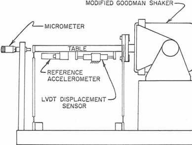
APPENDIX B - Development of a small shaking table for earthquake simulation

APPENDIX C - Magnetic and mechanical forces acting in the test accelerometers

123

1. INTRODUCTION

For about the last century, geophysical studies have been

aided by systems of sensitive instruments for the measurement of

earth motions. Set up in well supervised seismological stations

around the world, these instruments record continuously the faint

motions caused by earthquake activity throughout the earth. The high

sensitivities which rµake this long range monitoring possible

unfor-tunately prevent these instruments from giving useful data on the

strong motions associated with nearby earthquakes, since the

recorders then simply go off scale. This shortcoming has not been

considered to be of great importance for geophysical reasons since

nearby earthquakes are comparatively rare.

If local earthquake effects differed only quantitatively from

those recordable at greater distances, this attitude might still prevail.

It has long been suspected, though, that such is not the case, and that

the local effects which are responsible for the major economic impact

of large earthquakes are worthy of study in their own right. The

pursuit of this study soon led to the development of a new class of

instruments - strong motion seismographs.

Strong motion seismographs have to meet a number of rather

special requirements, the most trivial of which is reduced sensitivity

dictated by the very nature of their task: to give a good indication of local effects there should be at least several of them, spread over an area surrounding an earthquake epicenter. To have a reasonable probability of detecting an earthquake they must be located in as many as possible of the areas where earthquakes occasionally occur. Since the instruments must thus be rather numerous, they must be individ-ually relatively inexpensive. Since they must be spread over large areas, they cannot be continuously supervised, and must be capable of reliable automatic operation after long periods of sitting unattended.

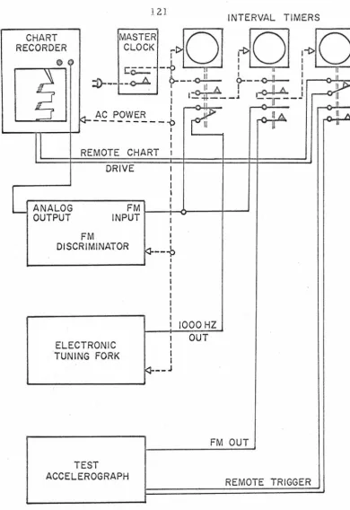
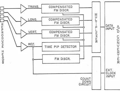
The numerous field instruments produce automatic records which are then analyzed at relatively few data reduction centers. Figures 1 and 2 show block diagrams of several such instrumentation systems either currently in use or undergoing active development. These systems differ considerably in their mechanical details, but they all show quite similar system organization and are subject to

similar analysis.

Each of the boxes in these two figures stands for a transfer operation, and each may be represented by a transfer function showing the relationship of input to output. Some parts of this relationship may be functionally described, e.g. frequency or impulse response of a viscously damped accelerometer. Others are best related in terms of statistical properties, e.g. distortion of photographic paper during chemical processing and drying. The product of all these

VECTOR ACCELERATION_ 3 AXIS ---it:>= l> ACCEL. VS TIME

~VERT

.

STARTER

h

OPTICAL

_.,,...

35mm t>-11 VELOCITY 11 VS Tl ME ACCELER-PHOTO. ..+- ENLARGE-~ MANUAL

-+-~ 11 DISPLACEMENT 11 VS TIME OM ET ER f- >-FILM MENT DIGITIZER COMPUTER I ~ SPECTRA ~---, RECORDER L_ --TIMING*

r->-~ STATISTICAL PROPERTIES

M0-2 (NEW

ZEALAND) *BRIGHTNESS MODULATION OF DATA TRACES VECTOR ACCELERATION . 3 AXIS ~ SPRING ~ ACCEL. VS TIME YvERT. STARTER

~

1

MECHANICAL P... 11 VELOCITY 11 VS TIME ~ DRIVEN PHOTO. ACCELER-WAXED ~ - ENLARGE-~ MANUAL ~ COMPUTER ~ 11 DISPLACEMENT 11 VS TIME OMETER

I-?-DIGITIZER I PAPER MENT b!-SPECTRA

·-

----e

RECORDER L -{ TIMING

l->

~ STATISTICAL PROPERTIES

SMAC-B (JAPAN) HORIZONTAL

HORIZ

.

STARTER

3

AXIS

OPTICAL ACCELER- OMETER

I

-

•

-

--A

TIMING 12 11 WIDE

PHOTO. PAPER .RECORDER

AR -240 VECTOR ACCELERATION 3 AXIS

w

··

OPTICAL

~

HORIZ . STARTER

t

ACCELER-1 O M ETER

I

.

-

' --~l TI M I N G RFT-250 VECTOR ACCELERATION

y

r 3 AXIS

~

HORIZ . STARTER

~J

ACCEL .

I

·-

-

-R M T-280

·

-TI M ING 8 FIELD INSTRU M ENTS

70mm PHOTO

.

FILM RECORDER _MAGNETIC

=i

TAPE RECORDER

DATA

--)-CONTROL

---1>

MANUAL DIGITIZER

ENLARGE- MENT F

M DISCRIM- INATOR I ~ I COMPUTER M ANUAL

DIGITIZER A/D CON- VERTER COMPUTER COMPUTER

ACCEL. VS TIME 11 VELOCITY 11 VS TIME 11 D IS PLACEMENT 11 VS

SPECTRA STATISTICAL

PROPERTIES

SAME SAME

on the right. Considerable work has been devoted to studies of the

data reduction area of these systems, comparing outputs at the far

right for a given record input to several data reduction systems,

but comparatively little has been done about the left half and

especially about box by box analysis of the overall system.

Studies of the right half of these diagrams have had their

effect on the left half, however, in that human judgment has been

identified as a principal variable in all of these systems, and that,

plus the sheer man-hours required for manual digitization of a

record of any length, has led to development of systems which

permit data flow from extreme left to extreme right with no

signi-ficant human intervention. An important step in this direction is

the development of magnetic tape recording instrumentation, and

this report is largely concerned with an analysis of such a system.

In analyzing the operation of an instrument system it is

necessary to keep in mind the information which is to be obtained

from it and the use to whiqh that information will be put. Presently

available systems produce acceleration/time records and response

spectra which are of great value in assessing possible damage to an

instrumented building following an earthquake, and for use in design

criteria for new buildings in a given area. They also may yield

statistical properties which are of value, for instance, in the

defining of model earthquakes for theoretical and experimental

studies of structure responses. And they produce 11

velocity11_/time

identify the mechanisms of strong earth motions.

The quotation marks around the words 11_velocity11 _and

11_displacement11

are significant. Presently used or considered

instrumentation systems are able to define velocities and

displace-ments only to within a long period component whose amplitude is not

accurately known and whose period may be as short as about one-half

the record duration. This uncertainty reflects to some extent the

lack of initial conditions in the records of existing instruments and

also the accuracy limits of the overall systems. It is of little

con-sequence in the parts of the response spectra curves which are of

interest in determining the response of most engineering structures.

But in

a

few cases, such as seiches in harbors and reservoirs, and

breakage of underground structures, it is a significant limitation. It

is also something of an impediment to studies of earthquake

mechan-isms, since it prevents any easy measurement of the grosser ground

motions associated with an earthquake.

One desirable direction for instrument development, then, is

in the direction of what might be called an "ultimate 11 _{instrument: one}

which is in effect a cross between the usual strong motion seismograph

and an inertial navigation system, and capable of recording the actual

motions in an earthquake with an uncertainty of an inch or so, rather

than many feet, and with corresponding improvements in the reliability

of the velocity and acceleration data. The basic system studied in this

report is capable, at least conceptually, of producing such performance

immense, as this study shows. The problems which stand in the way

of the improvement of current instruments up to the "ultimate"

system are indicative of the difficulty of development and probable

expense of any such system, barring an unforeseeable dramatic

2. ACCURACY CONSIDERATIONS IN STRONG MOTION EARTHQUAKE RECORDING

2. 1 Response of a Single Degree of Freedom System to a Transient Input Such as an Earthquake

The instruments traditionally used for earth motion recording are single degree of freedom, mass- spring-dashpot devices. The basic system with its equations of motion is shown schematically in the figure:

k

m

c

m

(x -

y)

+

ex

+

kx = 0

w =

Jk/m

= radian natural frequency 0

'

= c = fraction of critical damping 2Jkm

For a record starting at t = 0 with known initial conditions an integral solution of this equation is:

S

t

2

st sT

y(t) = y(O)

+

ty(O)

+

x(t)

+

Zw'

x(T) dT

+

w₀ x(s) ds dT

0

0 0 0

(1)

In seismic instrumentation, the motion y of the support is the ground motion, and the relative displacement x the measured quantity. Seismic instruments fall broadly into three categories, depending on the choice of

w

and

C •

These choices are reflected in the relative

0

importance of the last three terms in equation ( 1). When the instru-ment period is longer than the longest period in the motion y, the x term predominates (displacement meter). When the frequencies contained in y are near w and ' is several times larger than unity,

0

the middle term predominates (velocimeter). When the frequencies contained in y are all below w , the last term predominates

(acceler-o

ometer}. In common usage, strong motion instruments for earthquake engineering are nearly always of the accelerometer type, whereas seismographs for teleseismic use usually fall somewhere between the displacement and velocity classes. Some of the advantages of the accelerometer for strong motion use are:

(2) Accelerometers provide records which measure directly the quantity which is of primary interest to earthquake engineers.

From the acceleration-time record, response spectrum curves can be computed.

(3) Displacement meters have the difficulty that earth motions near earthquake epicenters sometimes reach amplitudes of a few yards. Such large relative displacements cannot be accommodated in an instrument of reasonable size.

(4) The sensitivity of velocimeters is critically dependent on the value of

C ,

while that of an accelerometer depends only on

w

0

Where a range of temperatures is involved, precise control of w 0

is relatively easy, whereas a corresponding precision in the control of

C

is much more difficult.

The transient response of a mechanical system may be written as:

t

x(t)

=

J

y(T)h(t-T}dT 0

where h(t) is the impulsive response. For a damped single degree of freedom system, initially at rest, this response is given by:

t x(t)

=

J

y{T)

0

e

-

w

e

(t - T)

.

r--:2

Slll W

where:

As a representative input function, y(t) will be taken as: N

y(t) =

l

an sin n;t

n=l

a = real constants

n

T = record duration

Substituting (3) into (2) gives

(3)

N -a.t t

x(t) =

l

an

T

J

(sin f3t sin m T cos f3Te O.T - cos f3t sin mT sin f3Tg.T)d T

n=l 0

where: a. =

woe

x(t)

where

f3 =

woJ1-c2

n'll"

m

= T

Performing the indicated integration then gives

N

=

l

an ( ₂ 1 _{2 2) { (} ps - Zm 2p )sm mt - Zmpa. cos mt

n= 1 f3 s - 4m f3

+ [ (ms - Zmp2)sm pt+ Zmpa. cos pt

J

e -a.t } (4)

For a typical strong motion accelerograph the exponentially

decaying terms in equation (4) are of little importance. Common

-1 -1

values are

s

= O.

6,

w

= 75 radians sec , so that a.= 45 sec . If

.0

the start-up time is . 1 seconds, which is also common, these terms

are already decayed to 1

% of their initial amplitude by the start of

the accelerogram, which is less than 1% of the remaining terms.

coefficients in a series of the form:

co

x ( t) =

l

b n sin n; ( t

+

Cj) n)

n=l and it will be found that

a /w 2

a

n n o

b

=

=

n

j

s2 - 4m2f32

(1

n2ir2 )

T2w 2

\ 0

(5)

4n2rr 2 _,2

+

T2w 2

(6)

0

The form of the denominator in the righthand side of equation

· (6) is the same as the well known steady state response of a damped

single degree of freedom system to a sinusoidal input at frequency

n rr

w

= T

From this it is clear that the Fourier amplitude

coef-..

ficients of x(t) may be made approximately equal to those for y(t), 2

to within the multiplicative constant w

0 , to any desired degree of

accuracy by proper choice of w₀ and ' to make the denominator

of b approximately 1.

n

Even if the denominator in equation (6) were always exactly 1,

the numerical value of y(t) would depend upon the variable phase shift

term in equation (5). This term has no effect on the Fourier amplitude

spectra, .but does modify the instantaneous acceleration values. This

effect can be minimized by taking ' """ 0. 7, which leads to an

approximately linear relationship between cp and n. In this case

n

the phase shift produces a simple time shift in the record, combined

with the already noted transient terms. For typical modern recorders,

which do not record the transient part of the response and have no

If displacements are to be calculated from the acceleration

vs. time record, though, the possibility remains that errors may still

be produced by the effect of double integrating the initial transients,

To investigate this possibility, assume that the denominators in

equation (6) are unity and multiply x by w 2 to get the recorded

0

acceleration. A measure of the displacement error would then be:

displacement error =

I

tst

w 2 x(t) dt - y(t) 2

0 0

°

Using equation (4) for x(t) and carrying out the algebra then gives:

displacement error

=

This error is non-decaying. For a typical term having a = 50 in/

sec~

n

n = 100,

C

= 0, 7, T = 50 seconds, and

w

= 75 rad/sec, the

coef-o

ficient is 0. 15 inches. The total effect depends on the particular

record considered, since the coefficients a as originally defined

n

can be mixed positive and negative and may either add or cancel. The

possibility exists, however, especially for long records, that a

significant difference could appear. Any such difference could be

eliminated either by applying the inverse transform of the mechanical

system to the record, if the transient part is included, or by taking

the value of

Clw

sufficiently small in the original design.

0

Ordinarily, other factors cause the accuracy of displacement

2. 2 Common Accelerograph Errors

The discussion so far has covered a few of the things which

must be considered in evaluating the processing of an accelerograph

record because of mechanical characteristics of an idealized

acceler-ometer. Real instruments are subject to departures from ideal

behavior which introduce additional factors. These departures may

be of great or minor consequence depending on the intended use of the

records. A few of the most significant ones follow, with estimates

of their effects on (1) instantaneous accelerations, (2) Fourier spectra,

and (3) the displacement calculated at t = 50 seconds.

Baseline Shift. Uncertainties in the record value corresponding to

zero acceleration can arise in many ways; for example,

acceler-ometer drift, record/playback errors, or simple lack of resolution.

For a baseline error consist,ing of a simple small translation:

(1) Instantaneous acceleration: error = shift. Typically not

significant.

(2) Fourier spectra: Ideally affects lowest order term only,

which is of no concern, but may have shorter period effects

through interaction with common computing techniques, one of

which is discussed briefly in Section 2. 3.

assumed linear, this error term may be treated independently of

the remainder of the signal. In this case a displacement error will

occur which reaches a maximum value at the end of the record and

is given by:

displacement error

=

1/2 (baseline error)T2

For a 50 second record duration and one inch permissible

displace-ment error, the permissible baseline error is 1. 2 x l0-6g, or about

• 0004% of 1/2 g full scale. This is several orders of magnitude

beyond the capabilities of existing recorders.

Instrument Tilt. If the instrument's orientation with respect to

gravity changes between the final in-place calibrations and the taking

of a record, a condition identical to the just mentioned baseline shift

will occur. It is mentioned separate! y here because of its special

consequences as regards ins.trument design. Tilts of the earth's

surface have been observed which were sufficient to close the starting

pendulums of AR-240 earthquake recorders and run out the paper

supply. That calculates to be in excess of . 002 radians, or sufficient

to produce a 50 second displacement error of more than 75 feet in a

horizontal accelerometer. The obvious conclusion is that instruments

intended for displacement computations must have means to nullify

such tilts, such as a servo leveling system, or perhaps use of

accelerometers which do not have true static response but rather are

Transduction Nonlinearities: If the overall transfer function of an

instrument system from accelerometer relative motion to playback is

nonlinear in a way which cannot conveniently be compensated for,

errors will result. The question is pertinent here because such

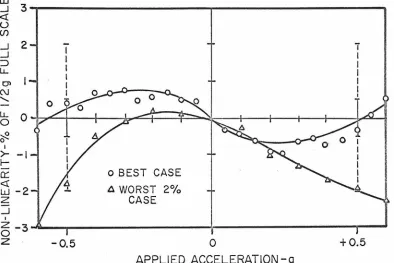
non-linearities have been observed in the RMT-280, which is the principal

subject of this report. (See Section 3. 5. )

(1) Instantaneous acceleration: Since the subject here is

trans-duction nonlinearities rather than mechanical nonlinearities, the

error at any level is simply the difference between the actual

instrument transfer function and the straight lin.e which is chosen

to approximate it.

(2) Fourier spectrum: The effect of nonlinearities on Fourier

spectra does not lend itself to easy, generalized analytical

representation. An estimate of the effect for small nonlinearities

may be obtained by considering one simple case involving an

unsymmetrical nonlinearity similar in nature to one which

some-times occurs in the RMT-280. (For purposes of this report, an

unsymmetrical nonlinearity will be defined as one which cannot be

approximated by a single straight line which is simultaneously

best for both positive and negative accelerations, e.g. one which

has significant even power terms in its power series expansion. )

Take the idealized case of a record consisting of a single

contains just a linear and a quadratic term:

y = A sin wt

..

y =y+

indicated

0 .• 2

Ymax y A

. A . 2

= sin wt +

o

s in wt

= A sin wt+ 0:

~A

sin 2 wt

(6)

For this simple case, the effect of the non-linearity has been to

introduce an additional coefficient into the Fourier spectrum at

twice the original frequency with an amplitude of the same order as

the per unit nonlinearity. The only general conclusion which

should be drawn from this is that Fourier spectra do not appear to

be critically sensitive to small nonlinearities in the range of

engineering interest. However, behavior remarkably similar to

this simple example was actually observed ,in the system tests

described in Section 4.

(3) 50 second displacement: A similar simplified example may

also be used to estimate the effect of nonlinearity on displacement.

An idealized earth motion consisting essentially of a step change

in displacement is shown in Fig. 3. The acceleration associated

with this idealized motion is a single cycle sine wave. A one second

period and an amplitude of 6. 28 feet second-2 would produce a

dis-placement of one foot. If this signal is subjected to the same

---~~~ ~ ~~~

...

..-~ ~ .,~ ~ ~~~~~~~~~~ ~~ ~~~~~~ ~~~~ ~ ~~ ~ I-.

t---..

. \ ...

---·.

. ·

DISPLACEMENT,

FT

1 r

·

.

...

.

··

0

2

term generated in the indicated acceleration will produce a

velocity error which leads to a displacement error which increases

linearly with time:

Yindicated - y"" (

0:/:

ft sec

-2)

(1 sec)(T sec)

~

If y. d" _{in ica e} t d - y

=

1 inch when T

=

50 seconds, then

oAT ft 2

0

= .

0004

=

• 04%. Extrapolated to 1 /2 g full scale, the permissible nonlinearity

grows to:

Y indicated - Y

y

=

o.

1%

The simple example chosen represents a worst case for an

unsymmetrical nonlinearity, but would produce at most a

displace-ment error of the same order as the nonlinearity (no velocity

error) for a symmetrical nonlinearity. This difference in

sensitivity is the reason for making a distinction between the two

kinds of nonlinearity. Both cases are applied to a more typical

record in the system tests of Section 4.

Cross Axis Sensitivity: There are two kinds of cross axis sensitivity:

The first is a small misalignment of the accelerometer sensitive axis,

so that the acceleration axes recorded are not quite in their intended

directions. The second is a change in the direction of the sensitive

axis as a function of applied acceleration, e.g. a pendulum

In the first case, the measuring error is given approximately by:

Yindicated - Y ~

y

where: = acceleration parallel to intended sensitive

axis

..

yJ_

=

acceleration perpendicular to intended

sensitive axis

e

= misalignment angle, radians

In the second case, for a pendulum accelerometer:

y - y

indicated

y

where: a.

=

sensing element rotation constant, radians

per unit acceleration (any consistent units),

When the angles are small enough that the quadratic terms may be

neglected, these errors may be related to the results for nonlinearities

by considering the special case where

y

_l =

Y.

11 • Then, for the first

case, the effect is a simple error in sensitivity, which can be thought

of as the simplest possible symmetrical nonlinearity. In the second

case, the per unit error is proportional to the applied acceleration,

which is precisely the unsymmetrical nonlinearity described just

above. For the test accelerometers, a. = • 016 radians/g, so the

Initial Conditions: Many practical problems stand in the way of

continuously recording strong motion instruments, and all instruments

now in use in the United States are of the stand-by type. Precise data

on the effect of mis sing the first part of the motion are therefore not

available. Some useful estimates can be made, however.

(1) Instantaneous acceleration: no effect.

(2) Fourier spectra: Comparative calculations for some specific

cases have shown that the omission of short sections of the

accelerograph record at the beginning and end of typical earthquake

records have negligible effect on the Fourier spectra (Reference 5).

(3) 50 second displacement: The pendulum starter used on USCGS

accelerographs has been developed empirically to do a satisfactory

job of separating significant seismic events from normal

back-ground motions. The starter in the RMT-280 was designed to have

the same dynamic characteristics. Half sine pulse tests on the

USCGS starter, reported in Reference 4, indicate that the initial

ground displacement at first contact closure is small, on the order

of 0. 05 inch, but .that initial velocities may easily be of the order

of 0. 5 inch/ sec. This velocity is small compared to the maximum

velocities encountered in an earthquake record, but is nevertheless

sufficient to account for a 25 inch error in the 50 second

Random Noise: Random noise can be added to an acceleration record

by reading errors in the case of photographic records, or by any of

a long list of noise sources in the case of electronic recorders. The

most important contributors to this problem in the test accelerograph

are described in Section 3. 2.

{l) Instantaneous acceleration: The uncertainty in this value is the

peak value of the added noise.

(2) Fourier spectra: If the sampling rate during digitizing is

sufficiently high so that the highest significant frequency

com-ponents of the added noise are below the Nyquist frequency, then

there will be errors in the Fourier coefficients whose maximum

magnitudes are equal to the corresponding coefficients of the noise

spectrum. If the Nyquist frequency is lower than a significant

component of either the noise or signal, then additional errors will

be generated by aliasing. One of the major advantages of an

all-electronic system is the practicality of removing unwanted high

frequencies by filtering and then using a sufficiently high sampling

rate to assure proper representation of the remaining information.

(3) 50 second displacement: The effect of random noise on

dis-placement calculations is a principal subject of Reference 6. In

where:

E{ X(T)} = x(T} S. D. { X(T) - x(T)}

X(T) = computed displacement x(T)

=

true displacement

T

=

record duration

cr

=

standard deviation of added random noise N = number of equally spaced samples taken

in time T

The conditions assumed in deriving these equations are satisfied by the present case of noise added to the signal before digitizing as long as the Nyquist frequency associated with N does not exceed the highest significant frequency component in the added noise. Higher values of N add no additional information, and so the assumption of independence of the samples breaks down,' and there is no

further improvement.

For a typical, carefully digitized, photographic record: = 0. 2 in/ sec2

T = 50 seconds

N = 500

S. D. { X(T) - x(T)} = 22. 4 inches For a typical RMT-280 record, filtered at 25 Hz (see Section 3. 2):

N

=

2500

S. D. { X(T} - x(T}} = 50 inches

The RMT-280 figure is somewhat worse than that for the optical

recorder but not as much as the higher noise level would lead one

to believe, and since neither figure is acceptable at this duration it

makes little real difference.

Time Base Errors: Time base errors may be conveniently divided

into two groups: the D. C. term, or average error, and higher order

terms in the Fourier expansion of instantaneous timing error vs. time.

For the D. C. term:

(1} Instantaneous acceleration: No effect on the actual peak values

of acceleration.

(2} Fourier spectra: Coefficients are unchanged, but all

fre-quencies are scaled by a percentage equal to the percent timing

error, e.g. timing standard 1 % fast will cause all frequencies to

belo/olow.

(3) 50 second displacement: For small errors there will be a

percent error in the final displacement equal to twice the percent

timing error, e.g. timing standard 1 % fast will cause computed

For the higher frequency terms:

(1) Instantaneous acceleration: Still no effect on peak values.

(2) Fourier spectra: This effect does not lend itself to easy

analytical representation, but some qualitative observations are in

order. When a change in the indicated rate of time flow occurs,

there is an apparent shift in all data frequency components exactly

analogous to frequency modulation of each data frequency. For the

case of a single data frequency and a single frequency variation in

the indicated time scale, an expression for the spectrum which is

generated by this modulation is derived in Reference 2:

M(t)

=

where: A

c

00

(

::c )

cos [(we

+

nw)t

+

~'IT

J

M(t) = modulated wave

Ac ·

=

data wave amplitude

we

=

data wave frequency

(7)

L::.w = amplitude of apparent frequency change due

c

to time base error

w = frequency of time base perturbation

v

When both the data signal and the time scale perturbation have

multiple term Fourier expansions, equation (7) becomes a triple

sum, and is too complicated to draw conclusions from easily.

(a) Since J

1 (z} ~ ~ , and higher terms higher orders, for

z

< <

1, the spectrum error is approximately two new terms

for each pair of interacting frequencies with resulting per unit

errors which are of the same order as the per unit time scale

variation.

(b) The spectrum is more sensitive to long period perturbations

than to shorter periods.

(c) It should be noted also that the effect of a change in the

speed of the recording medium which is not detected by the time

standard is exactly the same as the effect of an error in the

standard itself. This observation is particularly pertinent to

existing photographic recorders which provide time pips only

at intervals of one half second. Thus, chart speed variations

with periods of one second or longer may be detected and

corrected for, but shorter period components are not only not

properly accounted for, but will in general be illegitimately

reflected into the more sensitive long period part of the

spectrum by aliasing. This shows another great advantage of

the electronic recorder, in which it is practical to provide a

clock signal which operates at a frequency many times higher

than the highest frequency which will be used in any derived

Fourier spectrum. The result is an effectively continuous time

any mechanical recorder drive mechanism.

(3) 50 second displacement: The exact analysis of the effect of

random time base variations on displacement computations is

another problem whose complexity places it beyond the scope of

this report, but the remarks just made about discrete vs.

effectively continuous timing marks are equally valid here.

2. 3 Some Remarks on the Standard Baseline Adjustment Technique

As was mentioned at several points in Section 2. 2, there are

good physical reasons for believing that the mean value of the

acceler-ation during a typical seismic event is considerably smaller than the

values which would be calculated from unadjusted readings of the

accelerograms. It has become common practice, therefore, to apply

some sort of baseline adjustment to all accelerograph records before

data processing is attempted. The presently accepted standard

technique, which is described in detail in Reference 3, is, briefly:

where: a~:~(t) = adjusted acceleration

a(t) = recorded acceleration

co' cl' and c2 are constants chosen so that the

integral

I

T

[st~·-

]2

0 0

is minimized.

The coefficients generated are nonlinear functions of the original acceleration record, so that superposition may not be used in discussing the total effects of this correction technique.

Even though superposition is not strictly valid for this technique, it is possible to gain some insight into its operation by examining some highly simplified cases. For example, consider an unadjusted acceleration record which may be represented exactly by

a second degree polynomial. The adjusted acceleration from such a

record would be identically zero. This does not mean that the

adjusted acceleration is necessarily more accurate than the

unadjusted record, since the unadjusted record could conceivably have

been right to begin with. The adjustment process can not, of course,

provide any new information which was not contained in the original record. The example does indicate, however, that if a real record contained such a component, it would be reduced to a small value by the adjustment technique.

There are several ways in which such components may be introduced into a record, such as accelerometer drift, either

mechanical or electronic, chart paper distortion, and chart misalign-ment on a digitizing table. As indicated in Section 2. 2, the

sensitivity of displacement calculations to long period accelerations is such that amplitudes which are commonly found in unadjusted records, can lead to computed displacements several orders of

The adjusted records, in general, give displacements which are at

least physically reasonable, and so these records are certainly more

accurate than the unadjusted ones, even though the displacements may

still contain comparatively large errors.

An indication of the possible size and nature of these remaining

errors may be given by another simplified example. In Fig. 3 is

shown the acceleration, velocity and displacement associated with a

highly idealized ground motion, consisting of a single displacement

step (a fault slip, for example} which occurs in a short period of time

at the beginning of the record. Shown in broken lines are the shapes

which these curves would take if the acceleration record were adjusted

by the standard technique for two cases:

(1) Record length ten seconds {ten times duration of displacement).

(2) Record length fifty seconds (fifty times duration of

displace-ment).

From these curves, several observations may be made.

(1) When the duration of the displacement is an appreciable fraction

of the record length, errors of 50% or more in the computed

dis-placements are quite possible.

(2) The re is a tendency for adjusted displacements to fall toward

zero toward the end of the record, much as though a high pass filter

(3) Long, roughly periodic components are introduced into the

record. A quadratic correction in the acceleration will introduce

terms of the fourth degree into the displacement, with three

horizontal tangents possible in the record, and an associated

fundamental period on the order of one half the record duration.

This sort of behavior was also observed in the system tests

reported in Section 4.

(4) All of these effects are rapidly diminished as the record length

is increased. This behavior is in marked contrast to the effect of

a high pass filter, and suggests a reason for preferring this method

of adjustment. It also suggests the possibility of improving the long

period accuracy of records by allowing the recorder to run for

some time, say a minute or more, after large motions have

ceased. With photographic recorders, limitations imposed by

record storage capacity and digitizing man-hours made such

pro-longed recording impractical, but with tape recording devices such

as the test accelerograph, the idea seems worth further

investigation.

Until recording systems are developed which provide zero

point definition several orders of magnitude better than those now

available some form of baseline adjustment will continue to be

necessary. The current standard scheme has characteristics of

effectiveness difficult to prove, but it seems to serve well enough to

ensure its continued use. Even in the worst case, the errors in the

adjusted acceleration record are of the same order as the accuracy

limitations on accelerographs which are now in use or expected within

the next ten years. It must always be recognized, however, that

displacements computed from such adjusted records will contain long

period errors which may be quite large, no matter how good the

unadjusted record may be.

2, 4 An Idealized FM Seismographic Recorder

The preceding paragraphs have shown how zero line drifts and

lack of initial conditions in existing strong motion accelerographs can

lead to unacceptable errors in calculated displacements. In principle,

it should be possible to eliminate drift problems by producing an

instrument whose output is measured with respect to some standard

signal which drifts in the same way as the measured signal. In the

case of an FM system such as the test accelerograph, this can be

accomplished by providing a reference oscillator which is arranged so

that its drift characteristics are essentially the same as those of the

transducer oscillator. In such a case the phase differences only

become significant, and in addition a means is available for

deter-mining the initial velocity, as can be shown by an example.

Suppose that the signal applied to the recorder has a frequency

f modulated by an acceleration signal a(t) such that instantaneous

0

f = f

+

aa(t)

0

d8

=

dt

where 9 is defined by the instantaneous signal voltage, E:

E = E U(8)

0

U(8) is a periodic function of period 2'Jl" and unit amplitude (ideally

a sine wave, but not necessarily so).

Therefore

t

8

= f t

+

a

s

a(t) dt

+

e

0 0 0

If there is also available a reference oscillator running at f ' , it will

0

have

I I

8 = f t

+

9

0 0

and the phase difference between the two oscillators at any time will

be given by

e -

8

= (f - f )t I

+

8 - 80

+

a

Jt

a(t) dt

0 0 0 0

I

In the special case that f

0 = f0 and 80 = 80

I

8 - 8

t

=

a

J

a(t) dt

0

which differs only by the initial velocity, and the known constant a ,

from the system velocity. If, in addition, 8

=

e

at some time

shortly before the beginning of the recorded event when velocity is

zero, then the phase difference divided by a is precisely the system

continuously running and phase locking them together with a circuit

whose time constant is long compared to the anticipated record, so

that the average phase difference is zero when the average velocity is

zero for a sufficiently long period of time, say, several minutes.

An apparent ambiguity arises if the phase difference exceeds

'IT radians at the beginning of the record, since there is in general no

way to tell how many multiples of ±'IT radians separate the two signals

at that point. By proper selection of system parameters, however, it

may be arranged that this rarely happens and creates no difficulty

when it does. For example, if a

=

200 Hz/g (the value used in the

test accelerograph), then 'IT radians corresponds to 0. 5 f. p. s., which

is a velocity that would only rarely be exceeded within the start-up

time of presently known instruments. In the rare case that it was, an

error of 0. 5 f. p. s. in initial velocity would integrate to a displacement

error of 30 feet in a one minute record; that would surely resolve the

apparent ambiguity. The velocities associated with phase differences

less than 'IT radians are such that one might use some measure of

phase difference, such as instantaneous voltage difference between the

continuously running oscillators, as a means of triggering the recorder

into ope ration.

It is important to note that the phase difference between two

signals is independent of any irregularity in the motion of the recording

medium except skew, and skew effects may be eliminated if necessary

by multiplexing two signals on a single track. This system would

displacement, with an insensitivity to recording noise comparable to

digital techniques. At the same time, analogue acceleration playback

to satisfactory accu:i;-acy would be readily available by existing

techniques de scribed in Section 3. 2.

The purpose of this example is to show that a strong motion

accelerograph capable of providing meaningful displacement data may

be possible without the mechanical complexity and reliability problems

of continuous recording or the maintenance costs of large area

triggering networks. It is possible, at least in principle, with

existing recording techniques and stand-by type instruments, at the

expense of a relatively small continuous current drain. Problems

of long period drift in the oscillators are overcome by slaving the data

oscillators to the reference oscillator so that they all drift together.

The major obstacle to be overcome, at the present state of the art, is

an economically acceptable upgrading of the quality of the transducers.

The remainder of this report will concern itself in large degree with

3. TEST ACCELEROGRAPH ANALYSIS

3. 1 Instrument Description

The Earthquake Recorder studied uses electromechanical

transducers for the recording of strong motion earthquakes on

magnetic tape.

~:c

It is a battery powered recorder designed to sit

unattended in remote locations for periods up to several months, and

record earth motions above an adjustable threshold as they occur.

To achieve this endurance with a reasonable size battery pack, the

recorder was designed to be triggered into operation by the motion

itself, and to be turned completely off, drawing no stand-by power

whatsoever, between events.

A block diagram of the system has been shown at the bottom

of Fig. 2 in the introduction. In this block diagram, elements to the

left of the vertical double line are parts of the field instrument, while

those to the right remain in the laboratory or data reduction center

and are somewhat at the discretion of the individual user. A

description of the playback equipment used in this evaluation and the

considerations pertinent to its choice will be found in Section 3. 2.

The field instrument is an entirely self-contained unit

consisting of a three axis FM accelerometer package, a card

containing all control functions plus a fixed frequency reference

oscillator and an independent one-half second interval timer, a

magnetic tape recorder, an inverted pendulum starter, and a battery

pack, The physical arrangement of these elements is shown in

Fig. 4.

The accelerometer package contains three mutually

perpen-dicular Lehner-Griffith {Wood-Anderson) type accelerometers, each

with a moving coil in a permanent magnet field to provide both

damping and rough calibration, and a variable reluctance transducer.

The transducers are connected to three independent circuit cards

which produce electrical outputs which are a frequency modulated

analogue of the accelerations applied along the sensitive axes of their

respective accelerometers. The center frequencies are 1020, 1360,

and 1 700 Hz, with a deviation of 100 Hz equivalent to 1/2 g. These

accelerometers and their associated circuitry are described in greater

detail in Section 3. 3.

The control card contains relays for switching all circuits on

in response to a contact closure in the starting circuit, a time delay

which maintains power for 7 seconds after the last such closure, and

two independent timmg and reference systems. Provision is made for

starting from either the unit's own pendulum starter or from some

external source, such as another unit's pendulum starter or a relay

in a radio link. The timing and reference circuitry provides a fixed

frequency of 2040 Hz and an independent flip-flop circuit driving a

relay which amplitude modulates the 2040 Hz signal in a square wave

BATTERIES

WEATHER

COVER

N.A.B

.

TAPE

CARTRIDGE

MOTOR

INCHES

ACCELEROMETER

PACKAGE

[mr

1

1

1

rrrn

1 I

1

1 1

I1

11 l1

11

I1

1

1

I

1

1

1

I

1 11

!

1

11 l

1

1

'J

I

2

3

4

5

6

7

8

9

10

II

Figure

4:

Interior

View

of

Test

Provision is made also for driving this relay from an external source,

such as another recorder, in order to provide several recorders with

a common time base for correlation of their records.

The magnetic tape recorder uses standard NAB 1/411 _tape

cartridges with a capacity of 48 minutes at 3-3 / 4 inches per second.

Signals are recorded on four tracks, one for each acceleration

channel and one for the 2040 Hz reference. Use of separate tracks

permits recording in the direct mode with no bias. The FM

acceleration signals are recorded into saturation and the reference

signal just far enough below to preserve the amplitude variations

which carry the time pip information. The D. C. drive motor is

speed controlled by a mechanical governor and operates at twice

normal voltage to reduce start-up time.

The pendulum starter is dynamically equivalent to that used in

the original USCGS accelerograph. It is more compact that its

prede-cessors, but is virtually identical in performance, with a one second

period and approximately critical damping. It responds to inputs in

the horizontal plane, including static inputs such as instrument tilt.

The choice of period, damping, and contact clearance in this starter

probably is not in any sense optimized, owing to a marked scarcity

of design data (i. e. strong motion records which begin before the

arrival of the initial waves), but many years of operating experience

indicate that it performs its task of sorting out significant seismic

events from normal background motions with a high degree of

The battery pack consists of four 6-volt rechargeable batteries

giving 24 volts for recorder operation and± 12 volts for the solid state

electronics. The battery capacity is adequate for approximately 2-1/2

hours of continuous recording and the anticipated self discharge loss m

storage is less than 40 percent per year. After a year of inactivity,

the battery should have more than sufficient remaining capacity to use

up the recording tape.

. *

The analysis in this report is based on two accelerograph units ,

and on the first prototype of the FM accelerometer which is the basis

of the instrument.

3. 2 Short Period Noise Generation in the Accelerograph System

Unwanted and unpredictable low-level signals are generated at

every stage in the system, from the transducer itself through analog to

digital conversion of the magnetic tape records. Many noise sources

were identified in early testing and have been controlled by minor

redesign. In its present state, the system is capable of performance

closely approaching that of standard optically recording accelerographs.

The most natural division of noise sources in the system is not

by system components but rather by frequency, with a dividing line

placed at roughly one cycle per second. Above this frequency are

most of the problems associated with noise introduced by the recording

and playback process, analog to digital conversion, and mechanical,

~~

electrical and magnetic interactions between the various parts of the

field instrument. Below it are a collection of deviations from ideal

behavior which take place over periods ranging from several seconds

to several weeks and which are sufficiently distinctive in character to

be treated in a separate section. The phenomena associated with

start-up are roughly on the border in terms of frequency but fit more

naturally with the long period phenomena and will be included there.

The greatest single source of short period noise in the system

in its present form is the record/playback process. To appreciate the

sources of this noise, a brief digression into the state of the art of FM

tape systems is necessary.

An ideal FM discriminator may be considered as a device which

produces an output voltage proportional to the instantaneous frequency

of its input signal, and then subtracts a D. C. voltage to produce a null

output when the input is at the center frequency:

V(t) = Af(t) - Af = Alf

+

F(t)J - Af = AF(t)

o L 0 0

where V(t) = output voltage

A = a constant of the discriminator

f = center frequency

0

F(t) = a frequency function (departure from center

frequency) which carries the information

signal.

When the signal is recorded on magnetic tape as an intermediate

through the transport mechanisms at a precisely constant speed. If

the per unit speed variations are called a

1 (t) for the record pass and

a

2(t) for the playback pass, all frequencies in the original signal will

be multiplied by the quantity (l+ a

1)(1+a2) = 1 + a1 + a2 + a1 a2 =

1 + a.(t) . The output signal of the discriminator will be changed

correspondingly to

V'

=

A ( I

+

n(t) ) f ( t) - Af

0

=

n(t) Af 0

+

A ( I

+

n(t) ) F(t)

producing an error component or noise voltage:

I

V - V

=

a(t)Af + a(t) AF(t)

0

If a constant frequency f 1 is recorded on the tape at the same time as

the data signal f

+

F(t) and played back into a separate discriminator

0

set for that center frequency, a signal proportional to a(t) will be

produced ( F(t) = 0 in this case ) by means of which a degree of

compensation may be accomplished. The simplest technique is to

scale this speed variation signal to match the first term of the error

component above, and then subtract leaving only the second term. This

provides very good compensation for signals F(t) which do not deviate

very far from zero, but the quality of the compensation declines

rapidly as F(t) becomes an appreciable fraction of f .

0

A better technique, and the one which is used in the playback

equipment employed for this evaluation, is to use the speed variation

signal to control the gain of the data channel discriminator:

V '(t)

=

A' (n) ( I

+

n(t)) [ f

I

I

Then, if A (a.) = A

1

+

a.

v - v

= 0

It is possible, in principle at least, in this way to provide perfect

compensation for "flutter" (the name given to tape speed variations).

Circuits which accomplish the desired change in gain are available

and are not prohibitively complicated. A block diagram of such a

compensated system is shown in Fig. Al located in Appendix A.

Certain practical difficulties remain, however. In the output

circuitry of an FM discriminator it is necessary to provide a low-pass

filter in order to suppress the carrier frequency of the input wave.

A low pass 2nd order linear filter which is designed for minimum

distortion of complex wave forms has a time delay between input and

output which is nearly independent of frequency within its pass band

and whose magnitude is given approximately by:

where: ~t

Tr

~t

=

-...-zw--0

= time delay, seconds

W

0 = corner frequency, radians/ second

For example, the 25 Hz filter which was used ill the data channel of the

discriminator used for evaluation of the accelerograph system has a

delay of approximately 10 milliseconds.

Such small delays are significant because the compensation

compensation input of the data channel. It can be easily shown that

the result of such a delay is a residual noise signal which is

propor-tional both to the time derivative of the uncompensated noise signal

and to the time delay. With the 25 Hz filters originally included in

both channels of the discriminator system used in these tests, the

resulting transfer function, rising linearly with frequency, had unit

amplitude at 14 Hz, with noise frequency components higher than that

actually being amplified. Changing the compensation channel filter to

70 Hz corner frequency moved this unit gain frequency to 39 Hz and

improved performance considerably. Further boosts in the filter

frequency appear impractical due to beat frequencies generated when

the data and compensation carriers are allowed to mix. A large order

of improvement is still possible, however, by introducing a time

delay into the data channel, as indicated in Fig. Al. For reasons

which will be seen shortly, the total improvement from such added

complication is limited, and the system appears acceptable without it.

The RMT-280 system introduces a further complication into the

compensation problem by recording the reference signal and data

signals on separate tracks so that they do not necessarily see the

same instantaneous speed variations. The test accelerographs were

originally equipped with two head assemblies of two tracks apiece,

staggered vertically to produce four tracks on the tape. About an inch

of tape separated the point at which the reference signal was recorded

from that at which two of the three data signals were recorded. A

as . 01 lb rms could produce uncompensable errors greater than those

commonly accepted in previous optical recorders. Early testing

proved that excessive tape stretch did indeed occur and the final

version of the accelerograph has a single four element head. This

arrangement is still subject to errors due to tape skew, i. e. tape not

crossing the head at a constant angle, but this error has proved

experimentally to be acceptably small.

All such errors could be avoided by frequency multiplexing

a reference signal and three data signals on a single track, and this is

commonly done. The necessity of separating the four frequency

components applied on the track when the tapes are played back would

preclude the use of the present simple but highly nonlinear recording

process and add substantially to the complexity of individual field units.

Fortunately, this additional complexity is unnecessary in the present

instrument.

The noise output of the system was assessed by introducing

various signals into an FM discriminator and measuring the resulting

noise output with a B&K true RMS voltmeter set for a time constant of

10 seconds. In the case of noises generated within the instrument, a

single discriminator sufficed. In the case of noises generated by the

record/playback process a variety of combinations involving one

"data" channel and one compensation channel were tried.

All record/playback tests were made on the two head stack

version of the instrument. These tests provided the data which

included one set of tests which are val id for either case, so that it

was not necessary to repeat the tests when the heads were changed.

Test tapes were prepared by connecting all four heads of the recording

machine in series with a stable oscillator in order to record four

identical tracks which could then be used in various combinations as

data and compensation tracks. The normal arrangement of tracks

for both head configurations is shown in Fig. A2, Appendix A.

Play-back was always by the same machine: a Viking cartridge tape deck

which is similar in design to the RMT-280 transport mechanisms,

except that it uses a hysteresis synchronous AC motor in place of the

governor controlled D, C. one and has correspondingly better speed

regulation.

In some cases noise outputs were analyzed by passing them

through a Kron-Hite variable active filter used in the low-pass mode.

Band-pass filtering is a more conventional way of assessing noise

spectra, but filters of sufficiently narrow band width to be used in the

2-25 Hz range are not easily obtained, and the low pass filter used

has the advantage of being a realistic simulation of a possible actual

operating condition.

When it seemed desirable to obtain separate values for noise

sources which could only be measured in combination with other

noises, it has been assumed that the noises dealt with are

approxi-mately Gaussian so that their noise powers add algebraically. In

most cases the corrections obtained are of the same order as the

rather reasonable assumption is not critical. An example is the total flutter of the tape transport, which was obtained by deducting the

noise generated during playback from the total noise,

For convenience, noise values are reported as percentages of

1/2 g full scale. One percent thus corresponds to a one Hz frequency

deviation (100 Hz= 1/2 g).

The results of these measurements are summarized in Fig. 5

and in Table 1. The solid curves in the figure represent tapes

prepared on Accelerograph No. 1 and played back on the Viking deck.

Dashed curves represent tapes both prepared and played back on the

Viking de