Volume 8, No. 5, May-June 2017
International Journal of Advanced Research in Computer Science RESEARCH PAPER
Available Online at www.ijarcs.info
ISSN No. 0976-5697
Steganalysis on Images using SVM with Selected Hybrid Features of Gini Index
Feature Selection Algorithm
S. Deepa
Assistant Professor, Department of Computer ScienceGovernment Arts College Dharmapuri, Tamilnadu, India
R. Umarani
Associate Professor, Department of Computer ScienceSri Sarada College for Women Salem, Tamilnadu, India
Abstract: Image steganography techniques can be classified into two major categories such as spatial domain techniques and frequency domain techniques. In spatial domain techniques the secret message is hidden inside the image by applying some manipulation over the different pixels of the image. This work attempts to detect the stego images created by WOW algorithm by steganalysis on images, based on the classification of selected Hybrid image feature sets. It uses Gini Index as the feature selection algorithm on the combined features of the Chen, SPAM and Ccpev. The main scope of this work is to compete the previously implemented SVM-spam and SVM-HT methods. It uses the standard classification performance metrics to evaluate the performance of the three of the steganalysis models SVM-spam, SVM-HT and SVM-HG (SVM
1. INTRODUCTION
There are many categories of spatial domain techniques which differ mainly on the basis of manipulation of different bits in pixel values. Least significant bit (LSB)-based technique is one of the simplest and most widely used techniques that inserts or hides the secret message in the LSBs of pixel values without much visual distortion in the cover image. Another technique employs embedding of message bits at randomly chosen pixels. This technique is Pseudorandom LSB in which random pixels are chosen using algorithm where bits of secret data are embedded. Embedding average distortion or embedding change rate is the ratio of the changed bits in the cover image to the total cover image bits. It is well known that the lower the embedding rate the more difficult to detect the message.
with Hybrid features of Gini Index).
Keywords: Gini Index, Spatial Domain, Steganography, Steganalysis, SVM-HG
A. Drawback of Spatial Domain Steganography
The major drawback of these methods is amount of additive noise that creeps in the image which directly affects the Peak Signal to Noise Ratio and the statistical properties of the image. Moreover these embedding algorithms are applicable mainly to lossless image-compression schemes like JPEG, some of the message bits get lost during the compression step.
The most common algorithm belonging to this class of techniques is the Least Significant Bit (LSB) replacement technique in which the least significant bit of the binary representation of the pixel gray levels is used to represent the message bit. This kind of embedding leads to an addition of a noise of 0:5p on average in the pixels of the image where p is the embedding rate in bits/pixel.
A Simple LSB Steganography technique may have the following disadvantages
• Not vulnerable to different attacks.
• Intruder can easily guess and change the LSB's of the image pixels, thus original message gets destroyed.
• Causes some distortion in the original image.
• Scaling, rotation, cropping, addition of noise, or lossy compression to the stego-image will destroy the message.
But most of the modern spatial domain steganography methods claim that they will withstand against most of the common attacks.
2. AN EVALUATION OF STEGANOGRAPHY AND FEATURE EXTRACTION ALGORITHMS
A. Wavelet Obtained Weights (WOW)
V. Holub et al [1] presents a new approach for defining additive steganographic distortion in the spatial domain. The change in the output of directional high-pass filters after changing one pixel is weighted and then aggregated using the reciprocal Holder norm to define the individual pixel costs. In contrast to other adaptive embedding schemes, the aggregation rule is designed to force the embedding changes to highly textured or noisy regions and to avoid clean edges. Consequently, the new embedding scheme appears markedly more resistant to steganalysis using rich models.
B. Algorithms used for Feature Extraction
In this work, to design the steganalysis method, it uses three of the following different feature extraction algorithms. 1) Chen Features: Chen features are proposed by C. Chen and Y. Q. Shi in their paper “JPEG image steganalysis utilizing both intrablock and interblock correlations” [2] and “A Markov process based approach to effective attacking JPEG steganography" [3]. It presents an effective Markov process (MP) based JPEG steganalysis scheme, which utilizes both the intrablock and interblock correlations among JPEG coefficients. It computes transition probability matrix for each difference JPEG 2-D array to utilize the intrablock correlation, and "averaged" transition probability matrices for those difference mode 2-D arrays to utilize the interblock correlation. All the elements of these matrices are used as features for steganalysis.
detection of steganographic methods that embed in the spatial domain by adding a low-amplitude independent stego signal, an example of which is LSB matching. First, arguments are provided for modelling the differences between adjacent pixels using first-order and second-order Markov chains. Subsets of sample transition probability matrices are then used as features for a steganalyzer implemented by support vector machines.
3) Ccpev Features: Tomas Pevny et al [5] performed PEV features that are obtained by considering several different models for DCT coefficients and using the sample statistics of the models as features.
Despite the fact that calibration [6] has been shown to improve steganalysis, the authors are not aware of any study that would investigate its limitations and explain its inner workings on a deeper level. Moreover, there seem to exist some fallacies as to how calibration works. Though the principle is correct, this beneficial effect of calibration does not have to be solely due to the fact that the reference image provides an estimate of cover image features.
3. IMPLEMENTATION OF THE SVM-HT STEGO IMAGE DETECTION
A. About the Implementation
The Digital Data Embedding Laboratory Lab of Department of Electrical and Computer Engineering at Binghamton University, New York provides different implementations of steganographic algorithms for spatial domain, JPEG and Side Informed JPEG as well as some feature extraction methods in Matlab, MEX and C++. We developed our steganalysis model, we use the WOW steganography method, and three feature extraction methods. We will develop our steganalysis system in Matlab version 7 based on some of the source code of DDE lab [7].
B. Feature Selection using Gini Index
The Gini coefficient or Index is a measure of inequality developed by the Italian statistician Corrado Gini and published in his paper "Variabilita e mutabilita". It is usually used to measure income inequality, but can be used to measure any form of uneven distribution. The Gini coefficient is a number between 0 and 1, where 0 corresponds with perfect equality and 1 corresponds with perfect inequality. Equation (1) is the formula to calculate Gini coefficient.
Where, G: Gini coefficient
Xk: cumulated proportion of the one variable, Yk: cumulated proportion of the target variable, for k = 1,..., n, with Y0 = 0, Yn = 1
C. The Proposed SVM-HG (SVM with Hybrid features of Gini Index)
This work attempts the steganalysis on images which contain steganography by Wavelet Obtained Weights (WOW) Algorithm. This work only needs the message insertion part of the algorithm since it need some stego images for training and testing the proposed stego detection model.
The steps involved in this classifier are almost same as the previous work SVM-HT. The only difference is, instead of using t-test as in the previous work [8], this method uses a little bit improved Gini Index method for feature selection.
1) Steps of SVM-HG classification Method:
a) Input : WOW Stego Images and Non Stego Images b) Extract Chen-486,Spam-686 and Ccpev-548 Features of Non-Stego Images and Stego Images at Different BitsPerPixel (0.2 bpp, 0.4 bpp, 0.6 bpp, 0.8bpp)
c) The output is 3 set of features for Non stego Images and 4 set of features with stego images at 4 level of hiding for every feature extraction method.
d) For SVM-HG classification, combine the chen-486, Spam-686 and Ccpev-548 features of the non-stego image (from step 2) and the chen-486, Spam-686 and Ccpev-548 features of stego images at 4 level of hiding
e) Reduce the dimension of data (1720 features) using Gini Index feature selection algorithms and only use the first 1000 principal features from the combined feature dataset.
f) For k=1 to 10
g) Train the SVM neural network with randomly selected 70% of data mentioned in step e
h) classify the remaining 30% of data using the trained SVM network of step f
i) Performance(k)=Estimate the Performance() j) End
k) Find average performance from Performance(k)
4. THE RESULTS OF STEGANALYSIS AND DISCUSSION
A. About the used Image Database
The Images used for this evaluation were originally taken from the BOWS Image Dataset. BOWS (Break Our Watermarking System) was a Contest organised within the activity of the Watermarking Virtual Laboratory (Wavila) of the European Network of Excellence ECRYPT. Infact, the original dataset contains 10,000 images. But we have used a subset of cover images from BOWS database that were previously used in another work named “Gibbs Construction in Steganography [9]”. We used around 500 images to evaluate the performance of the proposed steganalysis model. We used cover images feature sets extracted using three different feature extraction algorithms. And we used stego images feature sets extracted using three different feature extraction algorithms at 4 different level of hiding such as 0.2 bpp, 0.4 bpp, 0.6 bpp and 0.8bpp.
B. The Metrics and Validation Method Used for Performance Evaluation
Classifier performance depends on the characteristics of the data to be classified. Performance of the selected algorithms is measured with metrics Sensitivity, Specificity, Accuracy, Precision, F_Score, and Error Rate. Various empirical tests can be performed to compare the classifier like holdout, random sub-sampling, k-fold cross validation and bootstrap method. The detection performance is also always averaged over several iterations.
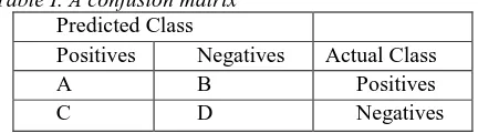
Table I. A confusion matrix
Predicted Class
Positives Negatives Actual Class
A B Positives
C D Negatives
The breakdown of a confusion matrix is as follows: • a is the number of positive examples correctly
classified (True Positives –TP)
• b is the number of positive examples misclassified as negative(False Negatives -FN)
• c is the number of negative examples misclassified as positive(False Positives –FP)
• d is the number of negative examples correctly classified(True Negatives –TN).
2) The Metrics:
a) Sensitivity / Recall: Sensitivity measures the proportion of actual positives which are correctly identified as such (e.g. the percentage of sick people who are correctly identified as having the condition). Sensitivity is also known recall. It is calculated using the following relation:
FN TP TP Recall y Sensitivit + = =
b) Specificity: Specificity measures the proportion of negatives, which are correctly identified (e.g. the percentage of healthy people who are correctly identified as not having the condition). It is calculated using the following relation:
FP
TN
TN
y
Specificit
+
=
c) Accuracy: Accuracy of a measurement system is the degree of closeness of measurements of a quantity to its actual (true) value. Accuracy is most commonly defined over all the classification errors that are made and, is calculated as:
FN TN FP TP TN TP Accuracy + + + + =
d) Precision / Positive Predictive Value: The Positive predictive value (PDV) or Precision is calculated using the following relation: FP TP TP Precision PPV + = =
e) F_Score: The f-score or f-measure is calculated using the following relation:
Recall
Precision
Recall
*
Precision
2
F_Score
+
×
=
f) Error Rate: The error rate is calculated using the following relation: FN TN FP TP FN FP rate Error + + + + =
g) Probability of Error: Generally, the detection accuracy is measured as the total probability of error under equal Bayesian priors
PE =1/2 (PFA + PMD ),
where PFA and PMD are the empirical probability of false alarm and missed detection respectively.
The error ratio can be considered as an approximate estimate of the error probability. Since the Error Rate is denoted as percentage, and the error probability should be between 0 and 1, the error rate is approximate in to error probability by scaling it between 0 and 1.
3) Cross Validation Method: Cross validation is a model evaluation method that is better than residuals. The problem with residual evaluations is that they do not give an indication of how well the learner will do when it is asked to make new predictions for data it has not already seen. One way to overcome this problem is, not to use the entire data set when training a learner. Some of the data is removed before training begins. Then when training is done, the data that was removed can be used to test the performance of the learned model on ``new'' data. This is the basic idea for a whole class of model evaluation methods called cross validation.
The holdout method is the simplest kind of cross validation. The data set is separated into two sets, called the training set and the testing set. The function approximator fits a function using the training set only. Then the function approximator is asked to predict the output values for the data in the testing set (it has never seen these output values before). K-fold cross validation is one way to improve over the holdout method. The data set is divided into k subsets, and the holdout method is repeated k times. Each time, one of the k subsets is used as the test set and the other k-1 subsets are put together to form a training set. Then the average error across all k trials is computed.
This work uses a variant of k-fold cross validation for validating the performance with respect to different metrics. A variant of this k-fold will randomly divide the data into a test and training set k different times and finding average performance. The advantage of doing this is that it allows to independently choose how large each training and test set is and how many trials to average over. It is equal to doing holdout cross validation for k times with random training and testing datasets and taking the average of that k trials, in each trial, this paper uses 70% data for training and 30% data for testing.
C. Table of Results
[image:4.595.120.477.95.272.2]The following are the numerical outputs of the performance of the classifier in terms of different metrics.
Table II. Performance of SVM-spam (spam686 Features)
Iteration Precision F_Score Sensitivity Specificity Accuracy Error
Rate
1 100.00 100.00 100.00 100.00 100.00 0.00 2 97.14 98.55 100.00 90.00 97.67 2.33 3 97.22 98.59 100.00 88.89 97.67 2.33 4 94.29 97.06 100.00 81.82 95.35 4.65 5 97.22 98.59 100.00 88.89 97.67 2.33 6 100.00 100.00 100.00 100.00 100.00 0.00 7 100.00 100.00 100.00 100.00 100.00 0.00 8 97.22 98.59 100.00 88.89 97.67 2.33 9 97.37 98.67 100.00 85.71 97.67 2.33 10 100.00 100.00 100.00 100.00 100.00 0.00
Avg 98.05 99.01 100.00 92.42 98.37 1.63
Table III. Performance of SVM-HT (First 1000 Feature provided by Ttest Algorithm)
Iteration Precision F_Score Sensitivity Specificity Accuracy Error
Rate
1 100.00 100.00 100.00 100.00 100.00 0.00 2 100.00 100.00 100.00 100.00 100.00 0.00 3 100.00 100.00 100.00 100.00 100.00 0.00 4 97.06 98.51 100.00 90.91 97.67 2.33 5 100.00 100.00 100.00 100.00 100.00 0.00 6 97.37 98.67 100.00 85.71 97.67 2.33 7 97.14 98.55 100.00 90.00 97.67 2.33 8 94.59 97.22 100.00 77.78 95.35 4.65 9 97.37 98.67 100.00 85.71 97.67 2.33 10 100.00 100.00 100.00 100.00 100.00 0.00
[image:4.595.123.477.483.735.2]Avg 98.35 99.16 100.00 93.01 98.60 1.40
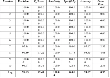
Table IV. Performance of SVM-HG (First 1000 Feature provided by Gini Index Algorithm)
Iteration Precision F_Score Sensitivity Specificity Accuracy Error
Rate
1 100.0 0
100.0 0
100.0 0
100.0 0
100.0 0
0.00
2 100.0 0
100.0 0
100.0 0
100.0 0
100.0 0
0.00
3 100.0 0
100.0 0
100.0 0
100.0 0
100.0 0
0.00
4 100.0 0
100.0 0
100.0 0
100.0 0
100.0 0
0.00
5 100.0 0
100.0 0
100.0 0
100.0 0
100.0 0
0.00
6 100.0 0
100.0 0
100.0 0
100.0 0
100.0 0
0.00
7 97.14 98.55 100.0 0
90.00 97.67 2.33
8 94.59 97.22 100.0 0
77.78 95.35 4.65
9 100.0 0
100.0 0
100.0 0
100.0 0
100.0 0
0.00
10 96.77 98.36 100.0 0
92.86 97.67 2.33
Avg 98.85 99.41 100.0 0
D. Performance of the Classifier or Stego Detection System
This paper compares the performance of the improved SVM-HG with the previous work SVM-HT and SVM-spam. The performance of SVM-chen and SVM-ccpev is not good as SVM-spam and so only scope of this work is to compete SVM-spam and SVM-HT.
Fig. 1 shows the performance of the stego image classifier or stego image detection system in terms of Error Rate. As shown in the figure, the proposed SVM-HG provided excellent performance than other two previously proposed models.
Figure 1. The Performance in terms of Error Rate
Fig. 2 shows the performance of the stego image detection system in terms of Accuracy. As shown in the figure, the proposed SVM-HG model provided excellent performance than other two previously proposed models.
Figure 2. The Performance in terms of Accuracy
Fig. 3 shows the performance of the stego image detection system in terms of Sensitivity.
Figure 3. The Performance in terms of Sensitivity
As shown in Fig. 3, all three proposed model provided excellent performance. Here high value of sensitivity signifies that the system was able to classify all the non-stego images correctly with much accuracy.
Fig. 4 shows the performance of the stego image detection system in terms of Specificity. As shown in the figure, the proposed SVM-HG model provided excellent performance than other two previously proposed models. Here high value of specificity in the case of SVM-HG signifies that the system was able to classify all the-stego images correctly with high accuracy.
Figure 4. The Performance in terms of Specificity
Fig. 5 shows the performance of the stego image detection system in terms of F-Score. As shown in the figure, the proposed SVM-HG model provided excellent performance than other two previously proposed models. Here high value of F-Score in the case of SVM-HG signifies that the system was able to classify all the stego images as well as non-stego images with high accuracy.
Figure 5. The Performance in terms of F-Score
Fig. 6 shows the performance of the stego image detection system in terms of Precision. As shown in the figure, the proposed SVM-HG model provided excellent performance than other two previously proposed models. Here high value of Precision in the case of SVM-HG signifies that the system was able to classify all the stego images with high accuracy.
Figure 6. The Performance in terms of Precision
classifier, (3) Ridge Regression, (4) LSMR Optimization and (5) LASSO. The results of the existing work are taken from the paper "Is Ensemble Classifier Needed for Steganalysis in High-Dimensional Feature Spaces? [10]”.
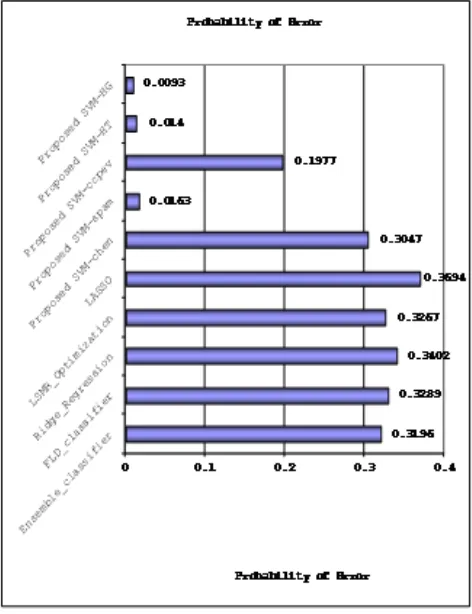
[image:6.595.39.275.379.686.2]Table IV shows the performance of proposed methods and previous methods in terms of probability of error.
Table IV: Performance in Terms of Probability of Error Sl.
No
Steganalysis Method
Probability of Error 1 Ensemble
classifier
0.3196
2 FLD classifier 0.3289 3 Ridge Regression 0.3402
4 LSMR
Optimization
0.3267
5 LASSO 0.3694
6 SVM-chen 0.3047
7 SVM-spam 0.0163
8 SVM-ccpev 0.1977
9 SVM-HT 0.0140
10 SVM-HG 0.0093
Fig. 7 shows the performance of proposed methods and previous methods in terms of probability of error. The performance of SVM-HG was very good and it provided very lower probability of error.
Figure 7. The Performance in terms of Probability of Error
The improvement in performance in the proposed model is due to the following four important aspects.
1) The use of SVM neural network based classifier. 2) The use of mixed class stego image features of images with different bpp hiding for training the SVM neural network.
3) The use combined extracted features from three state of the art feature extraction algorithms.
4) The use of Gini Index feature selection algorithm provided significant features.
5. CONCLUSION
All the three implemented steganalysis methods performed better than the compared existing works. But the performance of SVM-HG was very good and it provided very lower probability of error and outperformed all other compared algorithms with a significant difference in performance. The various experimentations show that the proposed approach is more effective and computationally efficient for all seven metrics. It is concluded that the Steganalysis performance of the proposed approach is significantly higher than the existing Steganalysis methods. The challenges between steganography algorithms and steganalysis methods were continuing for the last few decades. Up to now, there is a no winning, fool proof and safe steganography algorithms or steganalysis method. Novel sophisticated steganographic methods will require much novel feature detection methods as well as good feature matching approach for reliable detection. Targeted detection methods may provide reliable results. But there is no reliable method for guessing the stego algorithm for applying a particular targeted detection method. So, the universal blind detection methods are attractive and important research direction because of their flexibility to adapt to any new or unknown steganographic method. The future work is to address the application of suitable feature selection and feature reduction techniques to improve the classification performance of a steganalysis system.
REFERENCES
[1] V. Holub and J. Fridrich, "Designing steganographic distortion using directional filters", in Proc. IEEE WIFS, (Tenerife, Spain), Dec 2012.
[2] C. Chen and Y.Q. Shi, “JPEG image steganalysis utilizing both intrablock and interblock correlations”, IEEE ISCAS, International Symposium on Circuits and Systems, May 2008.
[3] Y. Q. Shi, "A Markov process based approach to effective attacking JPEG steganography", Information Hiding, 8th International Workshop, Springer-Verlag, New York, July 2006.
[4] Tomas Pevny, Patrick Bas, and Jessica Fridrich, “Steganalysis by subtractive pixel adjacency matrix”, IEEE Trans. on Info. Forensics and Security, 2010.
[5] Tomas Pevny and Jessica Fridrich, “Merging Markov and DCT features for multiclass JPEG steganalysis”, In E. J. Delp and P. W. Wong, editors, Proceedings SPIE, Electronic Imaging, Security, Steganography, and Watermarking of Multimedia Contents IX.
[6] San Jose, “Calibration revisited”, Proceedings of the 11th ACM Multimedia & Security Workshop, Princeton, NJ, Sep 2009.
[7] Database Reference: http://bows2.ec-lille.fr/
[8] S. Deepa and R. Umarani, “Steganalysis on images using SVM with selected hybrid features of Ttest feature selection algorithm”, UGC International Conference on Smart Approaches in Computer Science Research Arena, Jan 2017. (Article in a Conference Proceedings & in press)
[10] Remi Cogranne, Tomas Pevny, Vahid Sedighi and Jessica Fridrich, “Is ensemble classifier needed for steganalysis in high-dimensional feature spaces?”, IEEE International