Optical Information Storage and Processing

Processing

Thesis by Zhiwen Liu

In Partial Fulfillment of the Requirements for the Degree of

Doctor of Philosophy

California Institute of Technology Pasadena, California

2002

Acknowledgments

First of all, I would like to thank my advisor, Professor Demetri Psaltis. Without his patience, guidance and encouragement, I would not have finished this work. To him, my greatest gratitude.

Lucinda Acosta has provided tremendous help in almost everything during my stay in the group. I owe Yayun Liu so much for her generous assistance in the lab. Iouri Solo-matine has helped me a lot in making materials.

Many thanks to Dr. Greg Steckman for teaching me about the optical correlators and other lab skills when I joined the group. Thanks to Dr. Chris Moser for showing me how to use his spectral hole burning setup. Thanks to Dr. Wenhai Liu for all the interesting and productive discussions with him. Thanks to Dr. Ali Adibi for his encouragements and advice. David Zhang gave me great help in the spectral hole burning project as a surf stu-dent directly from high school. I would also like to thank George Panotopoulos for upgrad-ing me to "professor" every time I call him "doctor." Thanks to Jose Mumbru for his refreshing jokes. Thanks to Yunping Yang for coinventing a time-multiplexing technique when we were sharing the lab. Thanks to Irena Maravic for some heated philosophic debat-ing. I would like to thank Dr. Greg Billock, Dr. Karsten Buse, Dr. George Barbastathis, Dr. Gan Zhou, Dr. Xin An, Dr. Xu Wang, Dr. Ernest Chuang, Dr. Michael Levene, Dr. Allen Pu, Martin Centurion, Todd Meyrath, Hung-Te Hsieh, Manos Fitrakis, Marc Luennemann, Dimitris Sakellariou and all members of the extended Psaltis group family. I would also like to thank the secretaries of the EE department.

Optical information storage and optical information processing are the two themes of this thesis. Chapter two and three discuss the issue of storage while the final two chapters investigate the topic of optical computing.

In the second chapter, we demonstrate a holographic system which is able to record phenomena in nanosecond speed. Laser induced shock wave propagation is recorded by angularly multiplexing pulsed holograms. Five frames can be recorded with frame interval of I2ns and time resolution of 5.9ns. We also demonstrate a system which can record fast events holographically on a CCD camera. Carrier multiplexing is used to store 3 frames in a single CCD frame with frame interval of I2ns. This technique can be extended to record femtosecond events.

Information storage in subwavelength structures is discussed in the third chapter. A 2D simulation tool using the FDTD algorithm is developed and applied to calculate the far field scattering from subwavelength trenches. The simulation agrees with the experimental data very well. Width, depth and angle multiplexing is investigated to encode information in subwavelength features. An eigenfunction approach is adopted to analyze how much information can be stored given the length of the feature. Finally we study the effect of non-linear buffer layer.

We switch gear to holographic correlators in the fourth chapter. We study various properties of the defocused correlator which can control the shift invariance conveniently. An approximate expression of the shift selectivity is derived. We demonstrate a real time correlator with 480 templates. The cross talk of the correlators is also analyzed.

Table of Contents

CHAPTER 1 Introduction

CHAPTER 2 Holographic Recording of Fast Phenomena

2.1 Introduction ... 2-1 2.2 Nanosecond holographic movie camera ... 2-2 2.2.1 Nanosecond holographic system ... 2-4 2.2.2 Nanosecond movies of shock waves ... 2-8 2.3 Carrier multiplexing ... 2-12 2.4 Design of femtosecond holographic movie camera ... 2-21 2.4.1 Angular multiplexing in LiNb0_{3 . . .} 2-22 2.4.2 Wavelength multiplexing ... 2-28 2.4.3 Frequency multiplexing in spectral hole burning medium ... 2-29 2.5 Conclusion ... 2-37

CHAPTER 3 Diffraction from Subwavelength Structures

3.1 Introduction ... 3-1 3.2 Comparison ofFDTD simulation and IBM data ... 3-2 3.3 Encoding techniques ... 3-9 3.4 Eigenfunction analysis ... 3-17 3.5 Effect of nonlinear buffer layer ... 3-24 3.5.1 Perturbation method ... 3-25 3.5.2 FDTD and BPM simulations ... 3-28

3.7.2 Perfectly matched layer .... ... ... .. .... ... ... ... 3-40 3.7.3 Incident source implementation ... ... ... 3-47 3.7.4 Material modeling ... ... 3-51 3.7.5 Near field to far field transformation ... ... ... ... .. 3-55

CHAPTER 4 Defocused Holographic Correlator

4.1 Introduction ... ... .. ... .. ... . 4-1

4.2 Defocused holographic correlator array ... . .4-4 4.3 Shift selectivity ... ... ... .. .... .... ... .. ... 4-7

4.3.1 Gaussian process ... ... ... 4-8 4.3.2 Random binary pattern ... ... ... 4-11 4.3.3 Experiment. ... ... ... 4-12

4.4 Cross talk ... ... ... ... .. .. ... .... ... 4-17 4.5 Real time correlator system ... ... ... 4-20 4.6 Discussion ... ... ... .. .4-23

4.6.1 Incoherent correlator ... ... . 4-23 4.6.2 Information security ... .. ... 4-23 4.6.3 Spatial frequency domain representation .. ... ... .. .... 4-24

4.7 Conclusion ... ... ... .. ... 4-28

CHAPTER 5 Correlation Based Fingerprint Identification

5.1 Introduction ... ... ... 5- 1

CHAPTER 1 Introduction

CHAPTER 2 Holographic Recording of Fast Phenomena

Fig. 2-21. Femtosecond reference and signal pulse generators ... 2-18 Fig. 2-22. Signal pulse train ... 2-19 Fig. 2-23. Reflection grating ... 2-20 Fig. 2-24. Incoherent carrier multiplexing ... 2-21 Fig. 2-25. Experimental setup of femtosecond pulsed recording in LiNb0_{3 ..}... 2-22 Fig. 2-26. Recording and erasure curves ... 2-23 Fig. 2-27. Femtosecond pulsed hologram ... 2-24 Fig. 2-28. Selectivity curves ... 2-26 Fig. 2-29. Autocorrelation ofthe femtosecond pulse ... 2-26 Fig. 2-30. Comparison between theoretical and experimental selectivity ... 2-27 Fig. 2-31. Selectivity measured using He-Ne laser. ... 2-27 Fig. 2-32. Recording with chirped pulses ... 2-28 Fig. 2-33. Spectral hole burning medium ... 2-30 Fig. 2-34. Femtosecond movie camera ... 2-31 Fig. 2-35. Spectral hole burning holography experimental setup ... .2-32 Fig. 2-36. Bleaching kinetics ... 2-32 Fig. 2-37. Reading curves ... 2-33 Fig. 2-38. Angular selectivity (without iris filter) ... 2-34 Fig. 2-39. Angular selectivity (with iris filter) ... 2-34 Fig. 2-40. Angularly mUltiplexing plane wave holograms ... 2-35

Fig. 2-41. M/# measurement ... 2-36 CHAPTER 3 Diffraction from Subwavelength Structures

Fig. 3-25. Nonlinear absorption ... 3-33 Fig. 3-26. Yee cell ... 3-39 Fig. 3-27. Absorbing boundary ... 3-40 Fig. 3-28. Uniaxial perfectly matched layer. ... 3-42 Fig. 3-29. PML comer ... 3-45 Fig. 3-30. Introducing an incident wave ... 3-47 Fig. 3-31. Incident Gaussian beam ... 3-48 Fig. 3-32. Propagation of a 2D Gaussian beam ... 3-51 Fig. 3-33. Reflection from PEC and NiP ... 3-53 Fig. 3-34. Kerr nonlinearity ... 3-54 Fig. 3-35. Debye model ... 3-55

Fig. 3-36. Near field to far field transformation ... 3-56 CHAPTER 4 Defocused Holographic Correlator

Fig. 4-1. Holographic correlator array ... 4-2 Fig. 4-2. Correlation domains ... 4-3 Fig. 4-3. Defocused holographic correlator.. ... 4-4

Fig. 4-4. Selectivity function ... 4-8 Fig. 4-5. In-plane shift selectivity ... 4-13 Fig. 4-6. Out-of-plane shift selectivity ... 4-13 Fig. 4-7. Shift selectivity experiment setup ... 4-14

Fig. 4-12. Side lobe suppression in defocused corre1ators ... 4-18 Fig. 4-13. Cross talk in corre1ators ... 4-19 Fig. 4-14. Stored edge-enhanced template and its correlation output.. ... .4-20 Fig. 4-15. Correlation peak ... 4-21 Fig. 4-16. Correlation peak position ... 4-21 Fig. 4-17. Fingerprint correlation ... 4-22 Fig. 4-18. Face recognition ... 4-22 Fig. 4-19. Total power and correlation peak power ... 4-24 Fig. 4-20. Twin peaks ... 4-27 Fig. 4-2l. Effect of SLM displacement.. ... 4-28 CHAPTER 5 Correlation Based Fingerprint Identification

1

Introduction

Optics is one of the oldest fields in science, but yet it gives us fascinating new faces.

Optics has been found wide applications in physics (laser spectroscopy, quantum optics,

BEC, etc.), chemistry (femtosecond chemistry), biology (optical tweezers), and medical

practicing (laser eye surgery), to name but a few. The last two decades have witnessed the

revolution in the information industry: the boom of optical fiber telecommunications and

massive growth ofthe internet. However, the most widely used information processors are

still electronic (RAM, CPU). In this thesis we focus on the topic of information processing

using optical techniques.

One of the promising candidates for information storage is holographic memory. It

has attracted researchers' interest for decades because of its potential of huge storage

capacity (V/A3) and fast accessing rate (light speed optically, limited by electronics). In chapter two, we apply holography to monitoring fast phenomena. A reference pulse and a

signal pulse instead of two CW beams are used to record a hologram. Different frames are

recorded by different pairs of pulses using multiplexing techniques (angle, wavelength, and

frequency mUltiplexing). The resolution is limited by the recording laser pulse width. Indi~

vidual frames can be read out separately because of the multiplexing selectivity. A

nano-second movie camera is demonstrated, which is used to record the laser induced shock

wave propagation. The multiple pairs of recording pulses are generated from a single pulse

We also propose and demonstrate recording nanosecond events directly on commercially available low frame rate CCD cameras (30 fps) using carrier multiplexing. The femtosec-ond version of reference and signal pulse generators are designed. Carrier multiplexing can be extended to record femtosecond movies. Finally we propose another idea to build a fem-tosecond movie camera using spectral hole burning medium. Some preliminary material characterization of the SHB material (M/#) is included.

An approximate expression of the beam waist in the nonlinear medium is derived using a perturbation method. It is found that the waist depends on the effective nonlinear phase shift.

2

Holographic Recording of Fast Phenomena

2.1 Introduction

Monitoring fast phenomena is of interest to science and engineering since it tells us

about the dynamics of physical processes [2-1 ][2-2]. For instance, the pump-probe

tech-nique is widely used in non-destructive and repeatable measurements. For ID imaging

(e.g., lifetime measurements), streak cameras with subpicosecond resolution can be used.

Recording movies of fast events can be accomplished with a set of sensors [2-3]. The light

from the object is gated electronically on to each sensor (intensified CCD) while the image

is broadcasted. Limited by weak intensity and silicon circuit speed, about 10 frames can be

recorded with frame interval and time resolution of IOns.

Since the early days when holography was invented [2-4], people have been

study-ing high speed events usstudy-ing holographic techniques. A well known example is double

expo-sure interferometry [2-5]. In this method, two pulsed holograms are recorded successively

with the reference beams in the same direction. Upon reconstruction, the two frames are

reconstructed simultaneously and interfere with each other. Multiple frames can be stored

and reconstructed separately using multiplexing techniques. In Section 2.2 a system to

record nanosecond movies is discussed. We experimentally demonstrate the system by

making movies of laser induced shock waves with a temporal resolution of 5.9 ns, limited

by the pulse width ofthe Q-switched Nd:Y AG laser used in the experiments. In Section 2.3

we investigate carrier multiplexing on CCD cameras. We record three frames of an air

ond movies are investigated. Properties of femtosecond pulsed holograms in LiNb03 are discussed. Spectral hole burning holography is also investigated as a candidate to record femtosecond movies.

2.2 Nanosecond holographic movie camera

[2-13] [2-14]

Previous work has focused on spatial multiplexing where holograms are recorded at different locations of the recording medium. In an early report, a 100 ps laser pulse is used to store five frames [2-6). Beam splitters are used to generate the reference and signal pulse trains. The time delay between beam splitters determines the frame interval. In another method, a wave front preserving optical delay line (a White cell) and a specially graded beam splitter is used to generate the reference and signal pulse trains [2-7]. The frame interval can be as short as 28.3 ns. Spatial multiplexing by rotating the recording medium has also been reported [2-8], but the speed is either limited by the mechanical scan-ning or the laser pulse repetition rate. Pulsed holograms have also been angularly multi-plexed [2-9] taking advantage of the thickness of the recording medium. In one method, three lasers are used to generate three reference beams with different angles and each laser fires a pulse in a different time [2-10). The frame interval is about l).1s. A rotating mirror [2-11] or electro-optic switches [2-12] have also been used to generate the reference beams. In these efforts, the speed is limited by electronics or mechanic scanning.

is rotated) and thus it changes the perspective of the object. It also makes the interferometry between any two of the recorded frames more difficult.

The method we describe uses the angular selectivity of thick holograms to resolve frames that are recorded with adjacent pulses. Two specially designed cavities are used to generate the signal and reference pulse trains. The advantage of our methodis that the speed is limited by the pulse width of the laser instead of a scanning mechanism. The duration of the movie (the number of frames) is limited by the dynamic range of the recording material, not its spatial extent.

As shown in Figure 2-1, a sequence of signal and reference pulses are incident on

Hologram

Signal Fast changing object

Fig. 2-1. Angularly multiplexing pulsed holograms

the signal and the reference pulse trains are generated by a single pulse from a frequency

doubled Q-switched Nd:Y AG laser (wavelength 532nm, pulse width 5.9 ns, energy per

pulse 300 mJ, beam diameter 9mm).

2.2.1 Nanosecond holographic system

Figure 2-2 shows the cavity that generates the signal pulse train. A polarizing beam

Single pulse

I

I

J

Pockels cell Signal pulse train

1J4 w

aveplate

Fig. 2-2. Signal pulse train generation

splitter is used to couple the vertically polarized (perpendicular to the paper) incident pulse

into the cavity. The Pockels cell is timed to behave like a temporary "-/4 wave plate to rotate

the polarization of the incident pulse to horizontal direction after it first enters the cavity. It

is turned off afterwards while the pulse travels back towards the opposite mirror. The pulse

is then trapped inside the cavity since the polarizing beam splitter transmits beam with

hor-izontal polarization. A "-/4 wave plate is used to slightly rotate the polarization ofthe pulse

and the induced vertical polarized component is coupled out of the cavity from the

polar-izing beam splitter. A sequence of signal pulses are then generated and the pulse separation

is equal to the round trip time of the cavity. The two lenses inside the cavity form an

The reference cavity is shown in Figure 2-3. The incident pulse enters the cavity via Single pulse

Mirror

mm'or

Fig. 2-3. Reference pulse train generation

a small coupling mirror. After the coupling mirror, it travels as if it had originated from the center of the front mirror. The two lenses form an imaging system and the pulse hits the center of the rear mirror. If the rear mirror is parallel to the front one, the reflected pulse would travel backwards symmetrically with respect to the axis. After reflecting by the front mirror, it would then get blocked by the coupling mirror when it tries to retrace the previous path. We break the symmetry of the cavity by slanting the rear mirror slightly. The pulse is then reflected by the rear mirror and travels at a smaller angle towards the axis, just missing the coupling mirror. The pulse hits the center of each cavity mirror at slightly different angle after every round trip. Pulses are coupled out of the cavity by making one of the mir-rors partially reflecting.

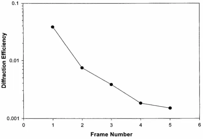
tion efficiency of each frame is shown in Figure 2-4. Both the reference and signal pulse

0.1 , - - - ,

>-u

r:::

.!!

u IE

w

r::: 0.01

o

..

u

~

i5

0.001 +---,---,---,---,---,---1

o

2 3 4 5 6 [image:22.540.103.447.129.365.2]

Frame Number

Fig. 2-4. Diffraction efficiency of pulsed holograms

train have a total energy of about 37 mJ. The pulse energy in the reference and signal pulse train decays and the successively recorded holograms get weaker and weaker. The diffrac-tion efficiency of the first hologram is 4% while that of the fifth hologram is about 10-3.

1.0

>-(.) c:

Q) '(3 _0.8

it:

W

c:

0 _0.6

~

(.)

co ~ It:

C 0.4

"C

Q)

,!::!

iU _0.2 E

~

0

Z 0.0

-1.5 -1.0 -0.5 0.0 0.5 1.0 1.5

Angle (degree)

Fig. 2-5. Angular selectivity

material dynamic range parameter. The M/# of the Aprilis material is about 6. Since we

typ-ically can obtain high fidelity reconstructions with 11 of 10-4, movies with several hundreds

of frames can be recorded.

We also recorded pulsed image holograms. A mask with random binary pattern was

used to modulate the signal beam. Figure 2-6 shows the reconstructed and direct images.

I-blogram Direct image

[image:23.540.120.432.101.325.2]

high power laser pulses. For this reason, a low quality mask was used.

2.2.2 Nanosecond movies of shock waves

We used this movie camera to record optical breakdown events. Our

single-pulse-pump-record experimental setup is shown in Figure 2-7. We split the pulse from the laser

Reference

----+-~1--t--1"

Generator

Recording

Materia~

Pocke~

Cell

Partially

Reflecting

J

Mirror

Signal Beam

Generator

1-- --,

! Polarizing Beamsplitter

I

A/2 waveplate

~ A!4 waveplate

and focus it on some sample. This pumping pulse can optically break down the object

[2-17]-[2-21]. Figure 2-8 shows the optical breakdown on a PMMA sample. Frame A is

~

.',

~'

, ,~

'* ," <$" 'M,

'"

.

A

D

,

, "J

\~"

'.

...

" "

.~'

"'*

B C

E F

Fig. 2-8. Optical breakdown in PMMA

recorded at about 1 ns before the pumping pulse vanishes. A, B, C, D and E are the

succes-sively recorded frames and the frame interval is about 12ns. F is the final direct image of

the sample after the optical breakdown. The size of the image is 1.74mm x 1.09mm. The

intensity of the pumping beam is about 1.6 x 1012W/cm2. Frame A shows the plasma

cre-ated by the pumping pulse. The tail is likely due to the discharge in the air in front of the

sample. In frame B, a shock wave is clearly seen. The average propagating speed of the

shock wave between frame A and B is about 10 km/s and that between frame D and E is

about 4 kmls. In Figure 2-9 we show the breakdown in air. Similarly, plasma is created in

frame A and soon a shock wave forms. The image size is 2.7 6mm x 1.17mm. The intensity

., .. ' " • If

-

.

'

,

:~.':

':, "

-.. .: :1'".

, ,

A B

the focal point of the lens and the length of that region is about equal to the depth of focus.

A line of spark is visible during the experiment. In Figure 2-10, we focus the pumping pulse

' f i't"

%/'" ;

~~

:

A B C

Fig. 2-10. Optical breakdown in air

near a blade (the dark rectangular shadow). The threshold of optical breakdown is lowered

by the presence of the metal blade. The image size is 1.82mm x I.4Smm. The intensity of

the pumping beam is about 1.6 x 1012W/cm2. The optical breakdown happens mainly at a

small region around the focal point which is close to the metal and produce a more spherical

shock wave. We also focused two pumping beams on PMMA to generate two shock waves

as shown in Figure 2-11. The image size is 1.48mm x I.S2mm. In the first movie the lower

pumping pulse has higher energy as we can see from the plasma size in frame 1 a. When the

two shock waves meet, the one with higher pressure penetrates as shown in frame 1 c. In the

second movie the two shock waves roughly have the same pressure, and they balance with

each other in the middle.

A unique feature of the holographic movie is that it records the field and thus has

both the amplitude and phase information. Phase changes can be detected by interfering

two reconstructed frames or interfering the frame with the reference wave. We interfere the

la Ib lc

2a 2b 2c

Fig. 2-11. Interaction of double shock waves

are shown in Figure 2-12. Apparently, the refractive index inside the region surrounded by

Fig. 2-12. Interferometry between a fast movie frame and its reference wave

the shock front is different from that of the outside and there is an index gradient. In the

holographic reconstruction we can focus at different depths since the object field is

recon-structed. This is shown in Figure 2-13. In A the plasma created on the PMMA sample is in

focus, while in B the shock wave due to the discharge in the air (in front of the sample)

[image:27.540.162.390.75.275.2]

pump-A

B

Fig. 2-13. Focusing at different depths

ing beam and the signal beam is about 20 degrees. The pumping pulse is focused at about 1 cm in front of the PMMA sample which is consistent with the measured image depth posi-tion difference between A and B.

2.3 Carrier multiplexing

[2-26]

The shock wave images in the previous section have low bandwidth. In principle we can also record these holograms in a thin medium. Because ofthe advancement of CCD technology, there has been a lot of interest in digital holography [2-22}-[2-2S] where holo-grams are recorded in a CCD camera and reconstructed digitally. CCD cameras not only provide a convenient interface to computers but also are an ideal thin recording material, which are sensitive to a very broad spectrum ranging from infrared to ultraviolet and have high responsivity (even hundreds of photons can be detected in one pixel).

beam-~~,LSJ

/

Fast changing object

---

,

Fig. 2-14. Carrier multiplexing

splitter is used in order to record holograms in Mach-Zehnder interferometer configuration. The CCD camera records the integration of the whole sequence of pulse exposure. All of the holograms are superimposed in one composite CCD frame and each can be indepen-dently reconstructed through digital spatial filtering if the image bandwidth of each holo-gram is sufficiently low. Individual holoholo-grams can then be filtered out and reconstructed by first performing a digital Fourier Transform on the composite image, filtering a selected pass-band corresponding to the desired hologram and then performing an inverse Fourier transform on the filtered result. As an example we consider the interference pattern shown in Figure 2-12, which is the hologram of an air discharge event. Figure 2-15a shows the DC filtered Fourier Transform. In general, the recorded pattern on the CCD is proportional to

a

Fig. 2-15. DC filtered Fourier Transform

which can be changed by changing the reference beam incidence angle. We filter out one

side band as shown in Figure 2-l5b and perform the Inverse Fourier Transform. Either R*S

or RS* is obtained. By taking the amplitude, the signal lSI is reconstructed as shown in

Figure 2-16. Different holograms can be recorded without overlapping with each other in

Fig. 2-16. Digitally reconstructed image

the frequency domain if the carrier frequency of each hologram is separated enough. The

typical bandwidth of an air discharge pattern is about 0.0024 f.lm-1. If the CCD pixel size is

10f.lm x 10f.lm (maximal bandwidth 0.05f.lm-1), hundreds of frames can be recorded and

reconstructed separately by 2D carrier multiplexing.

Our experimental setup is shown in Figure 2-17. We use the reference cavity in

[image:30.540.187.363.375.448.2]

imag-Nonpolarizing Beamsplitter

Polarizing Beamsplitter

A/2 Waveplate

Multiple Pulse Generation Cavity

, _{Coup mg} 1· M· _lITOr Fig. 2-17. Experimental setup

mg system and split into reference and signal by a non-polarizing beamsplitter. We recombine the reference and signal using mirrors and then record holograms on a CCD camera (Pulnix TM-7EX, 30 frames per second, 768 x 494 pixels, pixel size 8.4 x 9.8 )lm). A portion of the laser pulse is split off and focus on the signal path to induce the air dis-charge. Holograms of the optical breakdown in air are then recorded using this setup.

We generated three pulses with pulse separation of 12ns. Three plane wave pulsed holograms and the DC filtered Fourier Transform spectrum are given in Figure 2-18a and b respectively. Clearly, they are well separated in the frequency domain. We then recorded an air discharge movie. The holograms and the Fourier transform of the composite CCD frame are shown in Figure 2-19a and b respectively. We reconstructed the three holograms and the results are given in Figure 2-20abc. Because the holograms are recorded in the far field, the diffraction of the image needs to be compensated. Consider one of the holograms

*

calcu-a

b

Fig. 2-18. Plane wave holograms and their DC filtered Fourier Transform

a

b

Fig. 2-19. Air discharging movie

1ated by convolving the field at z=O with the Fresnel diffraction kernel, and is given by

[2-27]

(2-2)

We only need to multiply the reconstructed field by a chirped phase term and then perform

a b

c

d

e

f

Fig. 2-20. Digital reconstruction with and without diffraction compensation

image slightly from the center. The diffraction can be compensated by using a negative z

for Rj*Sj or a positive z for RjSj * term. The three frames after the diffraction compensation

are shown in Figure 2-20def. In the first frame (d) the plasma created by the optical

break-down in air is shown, while in the last two frames (e and f) a shock wave is formed and

propagates outward.

This method can also be extended to the femtosecond regime if a femtosecond

pulsed laser is used. A typical Ti:Sapphire mode locked laser has pulse energy of a few nJ.

Let us consider recording a movie using a single femtosecond pulse with InJ energy and

beam size of Icm2. We estimate that if the pulse uniformly illuminates the CCD, then each

pixel has about 4000 photons. Since we only need several hundred photons per pixel for the

recording of a single hologram, we expect that up to ten frames can be recorded with a

[image:33.540.59.482.75.296.2]

pules since the pulse is long (about 1.8 meters spatially). In the femtosecond regime since the pulse is very short (tens of microns spatially) we can simply use delay lines with thick-ness ofa few hundreds of microns. Figure 2-21 shows the reference and signal pulse

gen-Spectral domain Spectral domain

H---;~

~

\ : Delay line _{\ DelaYli'f}

Reference pulse generator Signal pulse generator Fig. 2-21. Femtosecond reference and signal pulse generators

the beam and all the pulses travel in the same direction. This set of pulses can then be used

as signal pulses.

As an example, we consider a femtosecond pulse given by

t2

f(t) = e -~e-j(j)ot where 0)0 = 2ltY

o = 2ltc _Ao (2-3)

We numerically simulate the generation of3 and 5 signal pulses shown in Figure 2-22. The

0.4 025

0.35

0.2

0.3

0.25

015

~

~

~ ~

I

0.2 .~

I

0.15 01

0.1

2.5

Time (f5)

Fig. 2-22. Signal pulse train

central wavelength Ao is chosen to be at 750nm and't is 100 fs. We uniformly divide the spectrum (Yo - _1 , Yo +

_1)

into 3 or 5 parts with the relative delay between neighboring

It't It't

pulses set to 5ps. The pulse width increases as we generate more signal pulses. There are also small ripples between pulses.

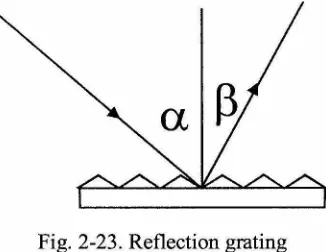
Let us now consider the angle separation of the reference pulses. As shown in Figure 2-23, the grating equation is given by [2-30]

Fig. 2-23. Reflection grating

which can be derived from the momentum conservation in the grating plane. K is the grat-ing vector and is given by

2n

K=m-A (2-5)

where m is the diffraction order and A is the period of the grating. For first order diffraction, Equation 2-4 can be rewritten as

"-A The angular dispersion is given by

sina - sinp

D =

IdPI

=

I

1

I

d,,- Acosp The angular separation between N reference pulses is 8 p

(2-6)

(2-7)

11"- P' where 11"- is the NAcos

wavelength bandwidth of the original femtosecond pulse. For a lOO fs pulse the bandwidth 11"- is about 2-3 nm.

*

is typically 1200 mm-l. This gives us 8p

~

0.03° for N=lO and

p = 60°. Bigger angle separation can be achieved ifP approaches to 90 degrees.

[image:36.540.195.358.76.202.2]

'\).b.~

<101>

_pv~

~

filter

bleachable material

a _b

Fig. 2-24. Incoherent carrier multiplexing

The two laser pulses interfere and produce an intensity pattern Iocos(qx). If the CCD has some sort of instantaneous intensity detection nonlinearity D[Iocos(qx)+I(x,y)], we can get a cross term I(x,y)cos(qx). We can again record fast events by changing the carrier fre-quency q with time. A possible implementation is given in b, where we illuminate two pulses on a bleachable material and form an instantaneous absorption grating cos(qx). The incoherent image I(x,y) is then modulated after transmitting the material. A filter is used to filter out the laser pulse. Again fast movies can be recorded by varying the carrier fre-quency.

2.4 Design of femtosecond holographic movie camera

The first scenario we will consider is angular multiplexing. We can directly scale the nanosecond system down using femtosecond laser pulses and shorter cavity length (or de1aylines). The major uncertainty here is the recording medium. If the image bandwidth is low, CCD cameras can be used as described in the previous section. In the following, we investigate recording femtosecond pulsed holograms in LiNb0₃ doped with Ceo The exper-imental setup is shown in Figure 2-25. The Ti:Sapphire mode locked laser is tuned to

Beam expander

4F system

, / Mirror G Al2 waveplate

Ce:LiNb03 _{Rotation stage ~} Polarizer

o

Achromatic lens

Fig. 2-25. Experimental setup of femtosecond pulsed recording in LiNb03

740nrn. The intensity of the reference and signal beam is equalized and is about 117m W / cm2. The recording and erasure curves are shown in Figure 2-26. Due to the short coher-ence length of femtosecond pulses, fanning cannot build up and we get a very clean record-ing curve which goes all the way to saturation. The gratrecord-ing strength A(t} is defined as the square root of the diffraction efficiency A( t} = JTl (t) .

Recording Erasure

0.04 , - - - . - - - , 0.04,---~

0.03 0.03

.c

0, c:

!!:!

.c

0, c:

!!:!

iii 0.02 Ol

(;) 0.02 Ol .E

i!!

c:

~

<.9 <.9

0.Q1 0.01

O.OO+---,-~-~-~-~-~~-6 8 10 12 14 o 10 12 14

Reoording time (hours) Erasure time (hours) Fig. 2-26. Recording and erasure curves

't Ao

using M# = Ao't~ and S = IL'tr [2-16][2-34]. 't_r and 't_e are equal unless the recording and erasure dynamics are characterized by a complex time constant, and in that case we should see oscillations in the recording curve. The difference of't_r and 't_e here is probably due to the short erasing time and error in fitting the erasure curve. We obtain M/# of 0.036 and S of 8.6 x 10-6 which are rather small.

Due to the short coherence length of the laser pulses, the hologram is recorded only in a thin slice of the material along the diagonal direction as shown in Figure 2-27. We assume that the laser pulse is given by E(t)=f(t)e-jot. The exposure energy P(x,y) is given as

P(x, y)

~ ~E(t

-

~

+

E(t-

~12

dt

~ ~(t

_

~ej~,

+

(t-

~ej~y

2

dt

(2-8)

~

f2

I

f

(t)1

2

dt

+

[ej~(,

- y)

f(t -

~

l(t -

~

dt

+ cc]

y

x

<,---Fig. 2-27. Femtosecond pulsed hologram

j~(X-Y)f£f

xl

*(

y)

j~(x-y)

(x-

Y)

iln(x, y) oc e C 1 \ t -

CJ

f t -

c

dt

+

cc

=

e C AC -c-

+

cc (2-9)

AC(t) is the autocorrelation function of f(t) and the thickness of the hologram is

determined by the coherence length (correlation length) of the laser pulses instead of the

thickness of the recording medium. Let's assume a Gaussian pulse.

[(I)

oc

ex+~:]

(2-10)

AC(I)

oc ex

p [ - 21:,]

j~(x-y)

(x-

y) jJ2~1;; (

Sl

[image:40.540.140.411.72.347.2]

where we rotate the (x, y) coordinate system 45 degrees to ~, s) system as shown in Figure 2-27.

(2-11)

U sing Born approximation and assuming the hologram extends to infinity along the ~ direc-tion, we can calculate the angular selectivity function.

f [

S2] [. 2sin888 J [ (88)2J

S(88) oc exp - c

2,/ exp J2n "A S ds oc exp -

if

where 88 is the angle change inside the material

~

=

J2

"A , "A&c are wavelength and speed of light in the material 2nc't

(2-12)

For external angle selectivity, we only need to replace ~ with n~ where n is the refractive index of the material.

After recording the hologram, we first use femtosecond pulses to read out the holo-gram and then tune the Ti:Sapphire laser to cw operation mode (at the same center wave-length) and read out the hologram with a cw beam. Figure 2-28 shows the angular selectivity curves. The selectivity curve of the pulsed readout is broader because different spectral component of the pulse Bragg-matches the hologram at slightly different angle. We measured the autocorrelation of the pulse using an autocorrelator. Figure 2-29 shows the measured intensity correlation IC(t)

=

flf(t')12If(t'

+

t)12dt' (equal to IAC(t)1 2 for a Gaussian pulse) and the fitted curve. The measured pulse width ('t) is 191 fs. The calculated selectivity is shown in Figure 2-30. They agree with each other very well. The selectivity

c 0 ~ ~ 8 0 "5

'"

"0 Q) .!::l OJ E (; Z [) c Q) ·u

IE _Q) c 0 . " ( ) J;l '6 "0 Q) .!::l OJ E (; Z 1.0 0.8 0.6 0.4 0.2 1.0 0.8

____ pulse readout

---6-cw readout

0.6

0.4

0.2

0.0 . . _ _ _ . . . ~--,--~ .... _ - _ - _ . . . -2.0 -1.5 -1.0 -0.5 0.0 0.5 1.0 1.5 2.0 2.5 3.0

Angle (degree)

Fig. 2-28. Selectivity curves

~

- fitted curve using y=0.0048+ 0.9798 x exp{-[(t-l.8994)/0.191]2}

•

Experiment

)

l

0.0

0.0 0.5 1.0 1.5 2.0

Time (ps)

2.5 3.0 3.5 4.0

Fig. 2-29. Autocorrelation of the femtosecond pulse

We also measured the selectivity using a He-Ne laser and the result is shown in

1.0 . , - - - . . . _ - - - ,

g

0.8 .91

u

=

(J)

5 0.6

~

~

'0

al 0.4

.!:! C6

E

~ 0.2

0.0 . . _ _ _ _ _ -~--.__-~--_ _ _ _ . . . . -2.0 -1.5 -1.0 -0.5 0.0 0.5 1.0 1.5 2.0

Angle (degree)

Fig. 2-30. Comparison between theoretical and experimental selectivity

1 . 0 , A

-()'

c 0.8

Q)

'0

!E Q)

§ 0.6 t5

(II

:t= '6

"C 0.4 Q)

.~

(ij

E

o

Z 0.2

0.0 . -. . . - -. . .

-~--.____-~--

. . . - . . . - ...

1.5 2.0 2.5 3.0 3.5 4.0 4.5 5.0 5.5

Angle (degree)

Fig. 2-31. Selectivity measured using He-Ne laser

[image:43.540.133.425.382.599.2]

energy of lmJ/cm2 can only yield a diffraction efficiency of 10-6 even if we assume that S=lcm/J is achievable in LiNb0_3. It would be very difficult to record a movie using a single femtosecond pulse from the laser.

2.4.2 Wavelength multiplexing

Femtosecond pulse has spectrum width of several nm and it makes wavelength mul-tiplexing possible. Shown in Figure 2-32 is a chirped pulse recording system. A

femtosec-!Tunable!

i Laser.

l _____ _

-._- --- -_. fs ns

Ti:sapPhire~pulse Spreader!~

• • • • • •

+~~+--7

Laser I 1 _ _ _ _

Sample

. --I I I

ICameral ! ___ J

[image:44.540.96.451.254.464.2]

Recording Material

Fig. 2-32. Recording with chirped pulses (courtesy of Dr. Gregory J. Steckman)

When M holograms are superimposed, it is well known that the diffraction effi-ciency of each hologram follows the M/# rule 11 =

(~#)

2 . M/# is approximately linear

in the material thickness M/#=(m/#)L where m/# is the per unit length. The wavelength

2

selectivity ofthe material is 8A

~ ~

. The spectrum of the pulse is f..A. Since the material cannot resolve wavelength difference smaller than 8A, M

~ ~~.

When we readout the pulsed hologram with a cw beam,

(2-13)

A2

where Lw = f..A is the coherence length of the pulse. In the case of a pulsed holo-gram recorded with two femtosecond pulses, this is consistent with the fact that the effec-tive thickness of the hologram is about Lw'

2.4.3 Frequency multiplexing in spectral hole burning medium

an absorption grating is recorded. An interesting feature of spectral hole burning medium is that it also has inhomogeneously broadened linewidth which is typically a few THz. This is because the local environment of the dopant differs from dopant to dopant and it affects the transition frequency as shown in Figure 2-33. We can think of the spectral hole burning

molecule

host

=

o

.-

-

e-o "-l

~

Fig. 2-33. Spectral hole burning medium

Frequency

not meet inside the SHB medium since the spectral components of the two pulses can still overlap both spatially and temporally. The problem of short coherence length of femtosec-ond pulses is also solved.

Figure 2-34 shows the femtosecond movie camera system using SHB medium. As

I

grating

I ,\

12 waveplate

I

mirror

II

PBS

t

lens

III

I

delayline

Cooled CCD

Fig. 2-34. Femtosecond movie camera

described in Section 2.3, multiple pulses can be generated by a single femtosecond pulse from the regenerative amplifier. Since each pulse has a different portion of the original spectrum we can use this sequence of pulses to record femtosecond movie in spectral hole burning medium. After recording, we use the low energy femtosecond pulses from the oscillator to read out the hologram. The pulses from the oscillator go through the same pulse shaping setup and individual frame can be read out by blocking all but one of the delaylines.

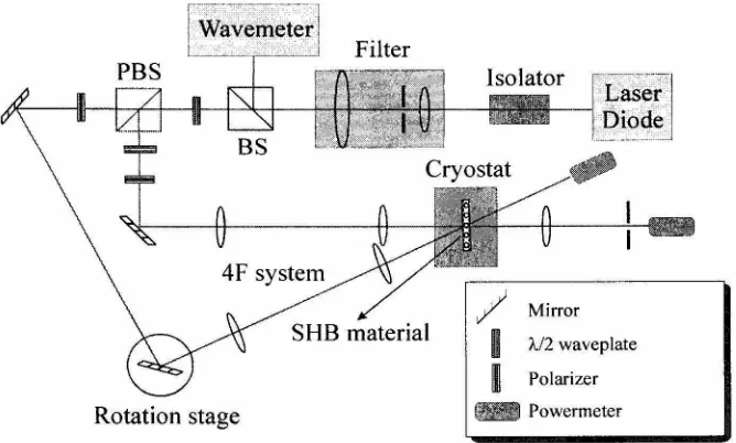
extended to other frequency channels. Figure 2-35 is the experimental setup. The sample is

4F system

SHB material

Rotation stage

Mirror

A/2 waveplate

Polarizer _ Powermeter

Fig. 2-35. Spectral hole burning holography experimental setup

put in a cryostat immersed with liquid Helium. Figure 2-36 shows the absorption kinetics

1.05 - , - - - , 1.00

0.95

>.

::;:; 0.90 c Q)

~ 0.B5 co

u

8-

O.BO

0.75 0.70

0.65

+---,---~--~---~--__,_---o 20 40 60

Time (8) BO

Fig. 2-36. Bleaching kinetics

[image:48.540.111.445.114.315.2] [image:48.540.138.420.419.622.2]

measured at 2 Kelvin. The bleaching beam intensity is about 10 ~W/cm2. The intensity

transmission coefficient satisfies T=exp(-2ad) where a is the absorption coefficient and d

is the thickness of the material. We define the optical density as OD = ad = -0.5InT .

Single plane wave hologram is recorded at different wavelengths by tuning the temperature

of the laser diode with both the reference and the signal intensity of 10 IlW/cm2.

Figure 2-37 shows the reading curves of the single plane wave hologram with the

unatten-3e-4

3e-4 - - A=788.42nm, Recording Time=1s

- - - A=788.40nm, Recording Time=5s

:>.

u

2e-4 c:

- A=788.4Bnm, Recording Time=15s

III 'u !E

w

c: 2e-4

0

13

~

1e-4

0

5&5

0

o 2 4 6 8 10 12 14 16

Reading Time (s)

p

Fig. 2-37. Reading curves

uated original reference beam. A diffraction efficiency of 10-4 can be consistently obtained.

The optimal recording time lies between 5-8 seconds. If we record for a longer amount of

time the material gets bleached everywhere (intensity modulation index <1). Due to the

oscillation of the cryostat we have difficulty to get consistent grating growth curves.

[image:49.540.138.438.246.509.2]

1.0

ift!t

~ _0.8

c::

Q) 'u

IE

t

!t

LU

c:: _0.6

0 n _III

:i=

!

0

lEft!

-0 0.4

ffttft

Q)

.!::! iii

E

0 0.2

Z

•

f~

·f

0.0

-2.0 -1.5 -1.0 -0.5 0.0 0.5 1.0 1.5 2.0

Angle (degree)

Fig. 2-38. Angular selectivity (without iris filter)

power meter (see Figure 2-35). The error bars stand for the standard deviation. The mea-sured selectivity is about 0.6 degree. However, the data is very noisy due to the scattering from the sample. An iris filter is then used at the back focal plane of the Fourier lens after

~ c:: Q) '0 !E LU c:: 0 ts til :i: is

5e-5

4e-5

3e-5

2e-5

1e-5

o

-1.0 -0.8 -0.6 -0.4 -0.2 0.0 0.2 0.4 0.6 0.8 1.0

Angle (degrees)

[image:50.541.133.423.438.647.2]

the sample. This serves for two purposes. One is to reduce the scattering and background

noise, and the other is to further reduce the selectivity. For thin material, if the reference

beam angle is changed slightly the reconstructed signal beam angle is changed accordingly

and can get blocked by the iris filter. The filter gives us a combined effect of both angular

Muttiplexing 3 holograms Muttiplexing 5 holograms

6&S 2.50-6

S&<; 2.0.<;

,.,

i:>

g ... c '.S&<;

" "

'0 '0

Ie Ie

w _3e-6 w _1.0.<;

c c

.g

11 u

~ ~

2&<> '!:; 5.<:&7

0 0

, ... 0.0

-5.00-7

-3 -2 -,

..

..

-2

Ange(degee) Ange(degree)

Muttipiexing 7 hologrMls Multiplexing 10 Holograms

1.2&-6 2 ...

1.0&-6

20-6

8.00-7

g-

g-" 6.00-7

" 'u

~ ,

...

Ie

W

4.~7 W

is c

ti .2 1) _50-7

~ 2.0e-7

..

:E

i5 i5

0.0

-2.0&-7

-4.0&-7

..

..

-50-7

-2 -8 -8

..

·2

Angle(degree) Angle (degree)

[image:51.541.76.479.191.559.2]

Figure 2-39. A selectivity of about 0.2 degree is obtained, which is consistent with the iris diameter of about 1 mm and the Fourier lens focal length of about 24cm. Three, five, seven and ten plane wave holograms are then multiplexed. After the recording, we scan the ref-erence beam angle and measure the dependence of the diffraction efficiency on the refer-ence angle. The obtained comb functions are shown in Figure 2-40. Because the readout process is destructive, a very coarse scanning is used. We use equal time (ls-2s) exposure schedule. Figure 2-41 shows the measured M/# of each case. As we multiplex 3, 5, 7 and

0.012

0.010

0.008

:l!: _0.006

:::2:

0.004

0.002

0.000

3 5 7 9

Number of multiplexed holograms Fig. 2-41. M/# measurement

[image:52.540.106.451.313.528.2]

From our experiments, about 10fJ,J/cm2 of exposure energy can yield a diffraction efficiency of 10-4 in one frequency channel. The spectral hole burning medium has high enough sensitivity to record tens of frames using a single pulse with energy ofmJs from the laser source if it has similar sensitivity during pulsed recording.

2.5 Conclusion

We demonstrate a nanosecond movie camera system by recording laser induced shock wave evolution. Five frames are recorded and the time resolution is 5.9 ns. Two spe-cially designed cavities are used to generate the reference and signal pulses and angular multiplexing is used to resolve holograms recorded successively. The movies we recorded are among the fastest ever recorded in 2D, comparable with the current state of the art of multi-camera systems (8 frames and IOns resolution). Holography provides the added advantages of recording 3-D and phase information. The sensitivity of holographic record-ing medium is an important issue in order to use the technique in shorter laser pulses or at different wavelengths. We propose and demonstrate carrier multiplexing in commercially available CCD cameras to alleviate the problem if the image bandwidth is low. We also investigate several scenarios to record femtosecond movies and frequency multiplexing in spectral hole burning medium seems to be a good candidate.

References

[2-1] Hyotcherl Ihee, Vladimir A. Lobastov, Udo M. Gomez, Boyd M. Goodson, Ramesh Srinivasan, Chong-Yu Ruan, and Ahmed H. Zewail. "Direct Imaging of Transient Molecular Structures with Ultrafast Diffraction." Science 291: 458-462 (2001)

[2-4] D. Gabor. "A new microscopic principle." Nature 161, 777 (1948)

[2-5] L.O. Heflinger, R.F. Wuerker, and R.E.Brooks. "Holographic interferometry." Journal of Applied Physics 37, 642 (1966)

[2-6] T. Tschudi, C. Yamanaka, T. Sasaki, K. Yoshida, and K. Tanaka. "A study a high-power laser effects in dielectrics using multi frame picosecond holography." Jour-nal of Physics D: Applied Physics Vol. 1 1 177-180 (1978)

[2-7] Michael J. Ehrlich, J. Scott Steckenrider, and James W. Wagner. "System for high-speed time-resolved holography of transient events." Appl. Opt. 31, 5947-5951 (1992)

[2-8] W. Hentschel and W. Lauterborn. "High speed holographic movie camera." Opti-cal Engineering 24, 687-691 (1985)

[2-9] P.J. Van Heerden. "A new optical method of storing and retrieving information." Appl. Opt. 2, 387-392 (1963)

[2-10] Shinichi Suzuki, Yasunori Nozaki, and Hiroshi Kimura. "High-speed holographic microscopy for fast-propagating cracks in transparent materials." Appl. Opt. 36, 7224-7233 (1997)

[2-11] R. G. Racca and 1. M. Dewey. "Time smear effects in spatial frequency multi-plexed holography." Appl. Opt. 28, 3652-3656 (1989)

[2-12] R. G. Racca and J. M. Dewey. "High-speed time-resolved holographic interferom-eter using solid-state shutters." Optics and Laser Technology 22, 199-204 (1990)

[2-l3] Gregory J. Steckman. Caltech Ph.D. thesis (2001)

[2-14] Zhiwen Liu, Gregory J. Steckman, and Demetri Psaltis. "Holographic recording of fast phenomena." Appl. Phys. Lett. 80, 731 (2002)

[2-16] Fai H. Mok, Geoffrey W. Burr, and Demetri Psaltis. "System metric for holo-graphic memory systems." Optics Letters 21, 896-898 (1996)

[2-17] Yu. P. Raizer. Laser-induced Discharge Phenomena (Consultants Bureau, New York, 1977)

[2-18] Roger M. Wood. Laser Damage in Optical Materials (Adam Hilger, Bristol and Boston, 1986)

[2-19] Y. R. Shen. The Principles of Nonlinear Optics (John Wiley & Sons, 1984)

[2-20] Hugo Sobral, Mayo Villagran-Muniz, Rafael Navarro-Gonzalez, and Alejandro C. Raga. "Temporal evolution of the shock wave and hot core air in laser induced plasma." Appl. Phys. Lett. 77, 3158-3160 (2000)

[2-21] Y. Tomita, M. Tsubota, K. Nagane, and N. An-naka. "Behavior of laser-induced cavitation bubbles in liquid nitrogen." Journal of Applied Physics Vol. 88 No. 10 5993-6001 (2000)

[2-22] E. Cuche, F. Bevilacqua, and C. Depeursinge. "Digital holography for quantitative phase-contrast imaging." Opt. Lett. 24, 291-293 (1999)

[2-23] G. Indebetouw and P. Klysubun. "Space-time digital holography: A three-dimen-sional microscopic imaging scheme with an arbitrary degree of spatial coherence." Appl. Phys. Lett. 75,2017-2019 (1999)

[2-24] S. Schedin, G. Pedrini, H.J. Tiziani, and F.M. Santoyo. "Simultaneous three-dimensional dynamic defonnation measurements with pulsed digital holography." Appl. Opt. 38, 7056-7062 (1999)

[2-25] S. Schedin, G. Pedrini, H.J. Tiziani, A.K. Aggarwal, and M.E. Gusev. "Highly sensitive pulsed digital holography for built-in defect analysis with a laser excita-tion." Appl. Opt. 40, 100-103 (2001)

[2-26] Zhiwen Liu, Martin Centurion, George Panotopoulos, John Hong, and Demetri Psaltis. "Holographic recording of fast events on a CCD camera." Opt. Lett. 27, 22-24 (2002)

[2-29] A. M. Weiner and Ayman M. Kanan. "Femtosecond Pulse Shaping for Synthesis, Processing, and Time-to-Space Conversion of Ultrafast Optical Waveforms." IEEE Journal of Selected Topics in Quantum Electronics 4, 317-331 (1998). [2-30] Christopher Palmer and Erwin Loewen. Richardson Grating Laboratory's

Diffrac-tion Grating Handbook (fourth ediDiffrac-tion) (http://www.gratinglab.com)

[2-31] Aleksander Rebane, Mikhail Drobizhev, and Christophe Sigel. "Single femtosec-ond exposure recording of an image hologram by spectral hole burning in an unstable tautomer of a phthalocyanine derivative." Opt. Lett. 25, 1633-1635 (2000)

[2-32] Kazutaka Oba, Pang-Chen Sun, and Yeshaiahu Fainman. "Nonvolatile photore-fractive spectral holography." Opt. Lett. 23, 915-917 (1998)

[2-33] Nils Abramson. "Light-in-flight recording: high-speed holographic motion pic-tures ofuItrafast phenomena." Appl. Opt. 22,215-232 (1983)

[2-34] Ali Adibi. Caltech Ph.D. thesis (2000)

[2-35] B. Plagemann, F. R. Graf, S. B. Altner, A. Renn, and U. P. Wild. "Exploring the limits of optical storage using persistent spectral hole-burning: holographic record-ing of 12,000 images." Appl. Phys. B 66, 67-74 (1998)

[2-36] S. Bernet, S. B. Altner, F. R. Graf, E. Maniloff, A. Renn, and U. P. Wild. "Fre-quency and phase swept holograms in spectral hole-burning materials." Appl. Opt. 34,22,4674-4684(1995)

[2-37] A. V. Turukhin, A.A. Gorokhovsky, C. Moser, I. V. Solomatin, and D. Psaltis. "Spectral hole burning in naphthalocyanines derivatives in the region 800 nm for holographic storage applications." J. Lum. 86, 399-405 (2000)

[2-39] Zhiwen Liu, Wenhai Liu, Christopher Moser, David Zhang, louri V. Solomatine, Demetri Psaltis, and Anshel Gorokhovsky. "Multiplexing and M# measurement in spectral hole burning medium." CLEO/QELS 2001, Baltimore, MD, May 2001

3

Diffraction from Subwavelength Structures

3.1 Introduction

Optical techniques have been widely used to store infonnation. The increasing

demand for higher storage density is constantly a driving force of research. Volume

holo-graphic memory has been of interest to researchers for decades due to its huge potential in

storage capacity and high speed accessing rate. Surface storage, such as DVD/CD

technol-ogy, has become more and more important recently because of its simplicity. The storage

density of these techniques is currently limited by the resolution of the light used to read

out the infonnation, i.e., the wavelength of the light source. Researchers have been able to

encode infonnation in the nanometer scale, but in order to read out the infonnation

compli-cated near field scanning is required. The main topic of this chapter is how to encode

infor-mation in subwavelength structures such that the difference of the scattering pattern in the

far field is drastic enough to be resolved.

In Section 3.2 we discuss the general properties of the diffraction pattern of

sub-wavelength structures. We compare the experimentally measured far field scattering

pat-tern from some trenches with our FDTD simulation results. We investigate several methods

to encode infonnation in Section 3.3 and analyze the general properties of such systems

using eigenfunction analysis in Section 3.4. In Section 3.5 we discuss the effects of adding

a nonlinear buffer layer on top of the layer encoded with infonnation. Finally, In Section

We developed a 2D simulation tool based on the FDTD algorithm which is briefly

reviewed in Section 3.7. In this section, we use the tool to calculate the far field scattering

patterns of some subwavelength structures (trenches) and compare them with the

experi-mental data. The fabrication of the trenches and far field scattering measurements were

done in IBM (3-1] [3-2]. The trenches were etched in NiP wafer which has a refractive

index of 2.07+j2.78 at A=633nm. They were probed by a focused He-Ne laser beam

(A=633nm, FWHM 5~m). Both the s (the electrical field parallel to the trench axis) and p

(the magnetic field parallel to the trench) polarizations were used. For each polarization,

two measurements were made with the incident angles (between the incident beam axis and

the sample normal) of 5 and 15 degrees. The profiles of the trenches were measured using

atomic force microscope (AFM) and we approximate the profiles in our simulation by

stair-case fittings with a resolution of 1../30. Figure 3-1 to Figure 3-4 show the comparison of the

simulation and the measured far field scattering. They agree with each other very well.

A common feature of the scattering patterns is that they have a peak on top of a

broad floor. When the probing beam is focused on the trench, it is first reflected by the

sur-face of the wafer. Light is also coupled into the trench and gets reflected by the bottom of

the trench. The peak is due to the reflection from the wafer surface while the reflection from

the bottom ofthe trench results in the broad floor because its spatial extension is limited by

the width of the trench. If the depth of the trench is close to 1../4, the two reflected beams

are out of phase and it produces two sharp dips where the floor meets the peak. We should

distinguish these two dips from the dips on the floor which are due to the far field

[image:61.543.68.487.229.590.2]

Profile 1 0,00

...

.

.

.

..

~

.

.

.

.

•

.

,< -0.01

2

~

~ -0.02

S

.

~

.

---

.

g. -0.03

" _•

.

··-l

-

Staircase fitling

J

• A.rS mea.SUfement -0.04

-0.05

-1.0 -0.8 -0.6 -0.4 -0.2 0.0 0.2 0.4 0.6 0.8 1.0

Transverse position ( normalized to A )

S polarization 5 degree incidence S polarization 15 degree incidence

,.<0

.?:-,~,

'iii

c:

~ 1e-2

,!;;

-0

Qi 1&-3

'"'

~ _.f!

.~ 1&-4 '0 <D ,

...

.~ "iii

E 1e-5

o Z Iii E 0 Z

.

...

~

,~, ,.~

18-7 +--~-~--~_~_~_~_~~_~_~_-I -1.0 -0.8 -0.6 .Q,4 -0.2 0.0 0.2 0.4 0.6 0.8 1.0

Sin(8)

P polarization 5 degree incidence

1e+O

.?:-'iii 1601

c:

~

,!;; ~ 1e-2

'"' .f!

~ 1&-3

Iii E o 1604

Z

1e-5

·',0 .0.8 -0.6 -0.4 ·0.2 0.0 0,2 0,4 0,6 0.8 1,0

Sin(8)

,.-<l

'~7

1e+0

~ 1e-1

c:

~

,!;; ~ 1e-2

'"' .f!

~ 1e-3

§

-0.8 ·0.6 -0.4 -02 00 0.2 0.4 0.' 0.8 '.0 Sin(8)

P polarization 15 degree incidence

1

- Simulation 1 • EJr:periment

o

Z 1~ 1~

10-5

..

~

·1.0 .0.8 .0.6 ·0.4 ·0.2 0,0 0.2 0,4 0.6 0,8 1.0

Sin(8)

1e+O

10-1

~

'"

c

.~ 10-2

:2

Q)

'"

~ 10-3

u

Q)

.~ (ii 10-4

E 0

z

10-5 10-6

-1.0 -O.B

1e+O

~ 10-1

'0; c

.~ 10-2

u Qi '" ~ 10-3

u

Q)

.~ (ii

1 &-4

E 0 ~.

•

Z 10-5 10-6

-1.0 -0.8

Profile 2

0.00 t----_:-,

-0.06

- Staircaseflttlng

.

..

• AFS measurement

~.

-0.08

L,--~~-~~--1.4 -1,2 -1.0 -0.8 -0.6 ·OA -0.2 0.0 0,2 0.4 0.6 0.8 1.0 1.2 1.4 Position ( normalized to A.. )

S polarization 5 degree incidence S polarization 15 degree incidence

1e+0 1e-1 ~ '0; c 10-2 2 .S "0 Qi 1e-3

•• "" _~

u _10-4

Q)

-~

(ii

E 10-5

0 Z

10-6 10-7

-0.6 -0.4 -0.2 0.0 0.2 0.4 0.6 0.8 1.0 -1.0 -0.8 -0.6 -0.4 -0.2 0.0 0.2 0.4 0.6

Sin(S) Sin(S)

P polarization 5 degree incidence P polarization 15 degree incidence

10+0 10-1

~

0; c _10-2

2

.S u

~ 10-3

~ u

.~ 10-4

(ii

E 0 10-5

Z 10-6 1e-7

-0.6 -0.4 -0.2 0.0 0.2 0.4 0.6 0.8 1.0 -1.0 -O.B -0.6 -0.4 -0.2 0.0 0.2 0.4 0.6

Sin(S) Sin(S)

Fig. 3-2. Profile 2 (experimental data from [3-1] [3-2])

0.8 1.0

[image:62.540.62.490.227.574.2]

"'" ·in c: Q) 5 u ~ .\!! u Q) .to! <Ii § z

"'"

in c: Q) .£; u Q) '" .l'! u Q) .to! iii E 0 Z 1e-1 10-2 10-3 10-4 '0-5 1e+0 Ie-I

1 ... 2

10-3

le-4

0.00 t---«ooo:-; -0,02

s

-8 -0.04

~ -0.06

1

-0.08

Z

-0.10

-0.12

Profile 3

-0.8 -0.6 -0.4 -0.2 0.0 0.2 0.4 0.6 0.8 1.0

Position (normalized to;q

S polarization 5degree incidence S polarization 15 degree incidence

-1.0 -0.8 -0.6 -0.4 -0.2 0.0 0.2 0.4 0.6 0.8 1.0 _{-1.0 -0.8 -0.6 -0.4 -0.2 0.0 0.2 0.4 0.6 0.8}

Sin(9) _Sin(6)

P polarization 5 degree incidence P polarization 15 degree incidence

1e+0

"'" ·in 10-1

[ - Simulation c:

• Experiment 2

.S

u ~ le-2 .l'!

u

Q)

.to!

iii

E le-3

0

Z

le-4

-1.0 -0.8 -0.6 -0.4 -0.2 0.0 0.2 0.4 0.6 0.8 1.0 -1.0 -0.8 -0.6 -0.4 -0.2 0.0 0.2 0.4 0.6 0.8

Sin(6) Sin(9)

Fig. 3-3. Profile 3 (experimental data from [3-1] [3-2])

1.0

[image:63.540.65.489.239.585.2]

~ ~ .5 ~ .!1! 'il .~ 0; § Z ?;-.;;; <= .!!! .5 '0 a; "" .l!! '0 " .t:! <0

E ₀ Z

Profile4

0.00

·0,05

t

·0,10

11

~

·(1.15

Z

·020

-0.25

-14 -1.2 -1.0 -0.8 -0.6 -0.'1 -0.2 0.0 02 0.4 0.6 o.a 1.0 1.2 1.4

Position (norma~zed to i.)

S polarization 5 degree incidence S polarization 15 degree incidence

'A", 18+0

llH

1.-2

'~3 ~

18-3

i

Z

-1.0 ..(l.S -0.6 -0.4 -0.2 0.0 0.2 0.4 06 0.' 1.0 -'.0 -0.8 -0.6 -0,4 -0.2 0.0 0.2 0.4 0.6 0.8 1.0

18-1

1e-2

1e-3

Sin(O)

P polarization 5 degree incidence

-1.0 -0.8 -0.6 -0.4 -0.2 0.0 0.2 0.4 0.6 0.8 1.0

Sin(8) 1e+0 ~le-' <= ~ l2 " ~ le-2

.l!!

~

a;

E ,.·3

o

Z

1 ...

Sin(8)

P polarization 15 degree incidence

·1.0 -0.8 ·0.6 -0.4 -0.2 0.0 0.2 0.4

Sin(8)

Fig. 3-4. Profile 4 (experimental data from [3-1] [3-2])

[image:64.541.68.489.230.573.2]

In profile 1, the trench is very narrow (0.4"-) and shallow (0.03"-). The two reflec-tions have little phase shift and there is no dip when the floor meets the peak. In profile 2,

the depth of the trench is about 0.07"- and again there is no dip when the floor meets the peak. However, the width of the trench is 1.6"-, and the far field diffraction of the light reflected from the bottom of the trench is approximately given by sinc(

wsi~S)

(Fourier transform of rect(

~)

), where W is the trench width. The diffraction produces a null (dip) at sinS

~ ~ ~

0.63 . In profile 3, the trench width is about 0.4"- and the depth is about 0.14"-. Because the trench is narrow it does not have any diffraction null on the floor, and more importantly, light cannot couple into the trench when illuminated with the s polarized light. Hence, the trench still appears shallow and there is no dip. However, if it is illumi-nated by the p polarized beam, light can couple into the trench and get reflected. The phase difference between the two reflected beams is significant enough to produce two dips. In Section 3.3, we will discuss the coupling to trench in more detail. In profile 4, the width of trench is 2"- and the depth is "-/4. The two reflections are out of phase and we see two sharp dips when the floor meets the peak. We also see the diffraction dips because the width is larger than the wavelength.

From the above analysis, we can simply model the wafer as a reflective phase mod-ulator. The phase change from the wafer surface to trench is controlled by the depth of the trench if p polarized probing beam is used or the width of the trench is large enough that s beam can also be coupled into it. We use profile 4 as an example. The near field of the scat-tering wave is approximately given as

-x: 2jkh[rect(

w)]

trench width and h is the trench depth. The far field is just the Fourier transform of the near field as given in Equation 3-113 or Equation 3-114. Figure 3-5 gives the results of this

1~---,~==============~

~

CJ) c::: Q)

-

c::: "0

~ 0.1

:m

_{ctI 0.01}

t>

CJ) "0 Q)

.!::::!

ctI

E

0.001 o

Z

_ Simple theory

- - Integral (obtained by Dr. Xu Wang) - - FDTD

0.0001 -JL----,,---,----r----,,---,----r---~-___r--__,__-__1j

-1.0 -0.8 -0.6 -0.4 -0.2 0.0 0.2 0.4 0.6 0.8 1.0

[image:66.540.75.483.189.476.2]

sinS

Fig. 3-5. Comparison of simple theory, FDTD and integral method

3.3 Encoding techniques

[image:67.541.57.483.462.679.2]

The trenches discussed in Section 3.2 can be modeled as waveguides as shown in

Figure 3-6. For simplicity, the wafer is assumed to be a perfect electric conductor instead

Fig. 3-6. Waveguide model

of NiP. The width of the trench is W. It is well known that there are three types of

waveguide modes, TE, TM, and TEM modes [3-4].

1. TE mode

(3-2)

where m=l, 2, ... and

P

(2:r -

c~r

.

The cut-off condition is

W

~ ~

.

2. TMmode

3. TEM mode (Oth TM mode)

(3-4)

The TEM mode is like a truncated plane wave and it always exists.

Figure 3-7 shows the calculated H (E) field at some instant t=to when illuminated

with p (s) polarized beam. The trench width is ')../3. When illuminated with the p polarized

beam, TEM mode can be excited in the trench. It propagates along the trench and is

reflected back. However if illuminated with s polarized beam, no propagating waveguide

modes can be excited and only some evanescent waves are excited.

In the following we discuss various schemes to encode information in

subwave-length structures using our FDTD simulation tool. We can encode information by varying

the trench width because it changes the ratio between the reflected wave from the wafer

sur-face and that from the bottom of the trench, and the waveguide mode cut-off conditions

depend on it. Figure 3-8 shows the far field scattering pattern of trenches with widths of')..

and ')../3 using both the sand p polarizations. The waist of the incident beam is 1.6')... The

depth is fixed to Al4. The wafer is assumed to be NiP. The far field scattering is different

for different trench width. Because the phase delay of the waveguide mode depends on the

depth, we can also encode information by varying the trench depth. Figure 3-9 shows the

far fields of trenches with depths of')../4 and ')..12. The width is fixed to').. in this case. The