Using Adversarial Examples in Natural Language Processing

Using Adversarial Examples in Natural Language Processing

Petr Bˇelohl´avek, Ondˇrej Pl´atek, Zdenˇek ˇ

Zabokrtsk´y, Milan Straka

Charles University, Faculty of Mathematics and Physics Malostransk´e n´amˇest´ı 25, Prague, Czech Republic

{belohlavek,oplatek,zabokrtsky,straka}@ufal.mff.cuni.cz

Abstract

Machine learning models have been providing promising results in many fields including natural language processing. These models are, nevertheless, prone toadversarial examples. These are artificially constructed examples which evince two main features: they resemble the real training data but they deceive already trained model. This paper investigates the effect of using adversarial examples during the training of recurrent neural networks whose text input is in the form of a sequence of word/character embeddings. The effects are studied on a compilation of eight NLP datasets whose interface was unified for quick experimenting. Based on the experiments and the dataset characteristics, we conclude that using the adversarial examples for NLP tasks that are modeled by recurrent neural networks provides a regularization effect and enables the training of models with greater number of parameters without overfitting. In addition, we discuss which combinations of datasets and model settings might benefit from the adversarial training the most.

Keywords:Neural networks, Adversarial examples, Natural Language Processing, Regularization, Evaluation

1.

Introduction

In recent years, deep learning has outperformed many of other machine learning models in various tasks of natu-ral language processing (Amodei et al., 2016; Wang et al., 2017; Yin et al., 2015; Collobert and Weston, 2008). Many of these models have been completely trained in end-to-end manner without any need for hand-crafting.

These models are usually very complex and tend to overfit easily, especially in cases of small datasets. For that rea-son,regularization techniquesare often employed in order to prevent overfitting. A popular solution to the lack of data and to model overfitting isdataset augmentation(Simard et al., 2003). This technique automatically generates similar training instances to the ones already present in the dataset, which effectively results in the dataset size increase. While augmenting the visual data is straightforward, the augmen-tation of text data is non-trivial.

Lately, a novel method for creating so called adversarial ex-amples was introduced Goodfellow et al. (2014b; Szegedy et al. (2013). These examples revealthat the models do not fulfil the smoothness assumption, i.e. the adversarial examples are very similar to the examples in the training dataset, but the already trained models classify them differ-ently than the very similar ones in the training data. When generating such examples during training and employing them in the process of model parameters update, they func-tion as strong regularizafunc-tion. Generating adversarial exam-ples can be understood as a form of dataset augmentation. The aim of this paper is to evaluate the effect of using the adversarial examples during training of the deep recur-rent neural networks which process natural language in the form of written text. More specifically, we intend to per-turb trainable word/character embeddings1_{(Mikolov et al.,} 2013) in a way the network is confused, although the new embeddings are extremely close to the original ones.

1

The vector representations of the text tokens which provide a unified input structure for machine learning models.

Our contribution is threefold:

• We prepared, selected and preprocessed a collection of eight distinct NLP datasets.

• Employing the collected datasets, we evaluate the ef-fects of using the adversarial examples during the deep learning model training. We include significance tests in order to support our claims.

• We discuss which datasets in general can benefit most from the adversarial examples.

2.

Related Work

Neural networks are commonly regularized by a handful of standard techniques. Apart from traditionalshrinkage tech-niquessuch asL2andL1regularization, the most used reg-ularization technique isdropout(Hinton et al., 2012) which randomly selects a subset of neurons that are disabled in a following training iteration.

Additional techniques include batch normalization (Ioffe and Szegedy, 2015) and layer normalization (Ba et al., 2016) which normalize the layer activation. Notably, re-current neural networks greatly benefit from the latter ap-proach. Further techniques include weight normaliza-tion(Salimans and Kingma, 2016),batch renormalization (Ioffe, 2017) andself normalizing networks(Klambauer et al., 2017).

Adversarial exampleshave been mostly studied in the con-text of image processing, especially for image classifica-tion. Goodfellow et al. (2014b), by following the work of Szegedy et al. (2013), show that not only highly non-linear models such as deep neural networks have adversarial ex-amples, but also much more linear and simpler models such as logistic regression do too.

affects various models trained on the same dataset. There-fore, the universality istwofold.

Nguyen et al. (2015) use a different approach by generating the adversarial examples by anevolution algorithminstead of by using gradient descent. This approach provides adver-sarial examples even in the environments in which the neu-ral network cannot be trained via back-propagation, since the target variables remain unknown.

Vidnerov´a and Neruda (2016) propose agenetic algorithm for adversarial example creation. They study robustness and generalization power of various models including both deep and shallow neural networks, support vector machines (SVM) even with radial basis function kernel (RBF) and decision trees.

Other noteworthy works regarding the adversarial examples in image processing include the work of Fawzi et al. (2016), Moosavi-Dezfooli et al. (2016b), Papernot et al. (2016b) and Papernot et al. (2016a).

Regarding adversarial examples used in the context of NLP, there is much less published research. Caswell et al. (2016) have been, to our knowledge, the first who exper-imented with using adversarial embedding perturbations. The IMDB dataset (Maas et al., 2011) was used as a bi-nary sentiment classification task. The authors introduced visualization techniques in order to understand the effect of constructed adversarial embeddings. Nonetheless, the re-sults of their experiments did not support any hypothesis of the method usefulness.

Miyato et al. (2016b) were the first who constructed adver-sarial perturbations of word embeddings. In addition, the authors employed a so-calledvirtual adversarial training which introduces a new loss term based on KL-divergence (Miyato et al., 2016b, Eq. 3,4). The authors evaluated five data sources and both adversarial and virtual adversarial learning outperformed the state-of-the-art models.2 Jia and Liang (2017) used adversarial generation of the source text instead of embeddings. They introduced var-ious methods fooling the models for Standford Question Answering Dataset (Rajpurkar et al., 2016) by generating additional sentences to the original source text.

Lu et al. (2017) aimed foradversarial examples detection in the context of Generative Adversarial Networks (GANs) (Goodfellow et al., 2014a). In addition, Miyato et al. (2016a) employed RNN-based GANs to semi-supervised text classification.

Adversarial examples are often created as a perturbation of the original input. Goodfellow et al. (2014b) and Szegedy et al. (2013) work with a deterministic perturbation which “damages” the current model the most. Contrary to them, using random perturbations has various theoretical implica-tions and is commonly employed (Matsuoka, 1992; Bishop, 1995; Grandvalet et al., 1997).

3.

Adversarial Examples

Adversarial examples are artificially constructed inputs that are very similar to some example from the training set, but

2

All experiments benefited from using a pretrained language model, which is a substantial difference from models used in our experiments.

they fool an already trained model. Adversarial examples can be employed during the model training in order to sup-ply new training data from which the model might benefit. Let us assume a classification task. Given a trained model representing functionf and a training example(x, y), the adversarial example is suchx+∆which fools the model, i.e. f(x) = y whilef(x+∆) 6= y. The difference∆

is called theperturbationand its magnitude can be limited subject to some metric. In our case, ∆ is a determinis-tic perturbation which is constructed subject to the gradient updates of the network.

We focus on NLP tasks in which the input is encoded as a sequence of word/character embeddings. The perturbation

∆slightly modifies the embeddings of the input sequence. The described process can be understood as a modification of the original example text, however, the final perturbed embedding does not correspond to a particular word (be-sides exceptional cases), since the perturbations are arbi-trary. Nevertheless, it is easy to find a nearest neighbor em-bedding and its corresponding word. Understandably, such nearest word does not necessarily behave the same as the perturbed embedding.

Since it is expected that the nearest neighbor is the original embedding without any perturbation applied, the adversar-ial examples in the context of NLP are difficult to interpret. One possible intuition is that the adversarial example re-places each word with a “new word” which is supposed to have a similar semantics to the original one, even though it is uninterpretable to human.

Apart from the proof of various machine learning models instability, Goodfellow et al. (2014b) demonstrated that employing the adversarial examples during the training of gradient-based models functions as a regularization tech-nique whose effect is comparable todropout(Hinton et al., 2012).

The main principle lies inonlinegeneration of adversarial examples throughout the training of the model. These gen-erated examples are similar to the training instances, which might improve model smoothness and generalization, by enforcing the model to behave similarly on a similar input (Goodfellow et al., 2014b).

This modification of the training effectively extends the training data, hence it can be understood as an augmenta-tion technique.

Given a training pair(x, y)and current model parameters

Θ, the cost functionJ might be linearly approximated on the neighborhood ofΘ.

Assuming the prior conditions, gradient∇ΘJ(x, y;Θ)can

Equa-tion 1.

∆=ε·sign ∇ΘJ(x, y;Θ)

(1) Goodfellow et al. (2014b) proposed a modification of the optimalization algorithm based on back-propagation which employs the adversarial examples.

The authors define a new loss function J˜which regards both the original loss and the loss computed on an adver-sarial example (based on the currently processed pattern). The definition ofJ˜for training pair(x, y)and parameters

Θ is given by Equation 2.

˜

J(x, y;Θ) =αJ(x, y;Θ) + (1−α)J(x+∆, y;Θ)

=αJ(x, y;Θ) + (1−α)·

·J(x+ε·sign(∇ΘJ(x, y;Θ)), y;Θ)

(2)

4.

Datasets

A collection of eight datasets in total was selected in order to evaluate the adversarial training in the context of NLP. In order to provide further complexity of the evaluation, we selected datasets that differ in multiple characteristics. However, due to limited resources, the selected datasets do not cover the whole characteristic space.

All datasets were provided with a unified interface so that they could be easily experimented with.3

At first, we selected three of the Facebook bAbI datasets (Weston et al., 2015; Sukhbaatar et al., 2015). Each of the datasets models a different aspect of natural language understanding and reasoning. The typical dataset example contains a sequence of facts regarding position of various objects and a question testing the understanding and rea-soning based on these facts. To be specific, we decided to choose the English versions of bAbI tasks #1, #2 and #6, because they represent both simple and advanced problems. Secondly, we focused on subjectivity detection, i.e. distin-guishing between subjective and objective texts. For this reason, we selected Movie Review Data (originally evalu-ated by Pang and Lee (2004)). This dataset contains short texts (typically single sentences), which were automatically mined either from the official movie description provided by the distributor or from the user reviews. It is assumed that the prior texts are objective and the latter subjective. This process of automatic mining naturally introduces a noise in the generated annotations, i.e. some objective sen-tences are probably classified as subjective and vise-versa. In order to evaluate also non-English datasets, we selected three Czech/Slovak datasets. All of them aim to test senti-ment analysis, i.e. the goal of the model is to distinguish among positive, negative, bipolar and neutral texts. The three selected datasets (Social Media Dataset, Movie Re-view Dataset and Product ReRe-view Dataset, all described by Habernal et al. (2013)) represent texts regarding various topics and were automatically collected from the internet.

3_{We implemented and employed deep learning framework} cxflow (v0.4) for all our experiments (https://cxflow.org) as it supports quick experiment creation, logging and result man-agement.

Their sentiment was automatically derived based on the rat-ing assigned to the reviewed item (number of stars). The final selected dataset is the one introduced as Discrimi-nating between Similar Language (DSL) Shared Task 2015 at LT4VarDial - Joint Workshop on Language Technology for Closely Related Languages, Varieties and Dialects in 2015 (Zampieri et al., 2015). The goal of the dataset is to demonstrate the language discrimination among 13 differ-ent languages and dialects and one additional category. The provided dataset contains approximately 200 thousand ex-amples, which enable us to restrict the training set to a spec-ified number of examples. We use the restricted versions of this dataset in order to evaluate the effects of various dataset sizes on adversarial training.

In order to evaluate the effect of adversarial examples, we consider the following dataset features that aim to cover distinct types of NLP datasets. We use the characteristics for discussion of the relation between the regularization ef-fect of adversarial examples and the dataset features.

• Dataset size: number of the training examples. • Dataset language: input text language. • Vocabulary size: number of distinct tokens.

• Text length: distribution of the text lengths in the train-ing dataset.

• Annotation quality: noise amount in the gold labels. • Input text structure: distribution of the token

fre-quency; number of sentences.

• Dataset artificiality: real-world dataset vs. artificially constructed one.

5.

Evaluation

Each dataset was split into three distinct parts: training, validation and testing. The training part was used for the model parameter estimation, the validation for the best model selection and the testing for the final result reports. We employ the testing losses in order to perform signifi-cance of the performance improvement.

5.1.

Model Selection

The neural networks are typically trained in several epochs. After each epoch, the model loss is evaluated both on train-ingandvalidationdata. While the validation loss represents an independent estimation of the model generalization ca-pability, both losses are used together for overfitting detec-tion.

In order to select the epoch in which the model achieved the best performance, we select the one in which theloss was the leaston the validation data. The final performance is then reported ontestingdataset, which is completely held-out until the final model is selected.

Since the validation and test datasets were constructed by randomly choosing examples, the test performance on the model isconditionally independent on the validation per-formance given the model parameters. However, the test performance is expected to be slightly worse in comparison to the validation performance since the model was chosen to achieve the best validation performance regardless the test evaluation.

models the actual behavior of the model. In contrast, in a classification problem, the accuracy of the model does not express its behavior in a sufficient detail.

5.2.

Testing Significance

In order to evaluate whether the adversarial training has a significantly positive effect on model performance, we per-form thepaired t-teston the testing losses as follows. Comparing two experiments given a single dataset, we train appropriate network architectures independently with the same train/valid/test data split. Then, we select the best models using the validation dataset. Finally, we evaluate and compare the testing losses between the corresponding testing examples. This leads to a paired t-test using these two sets of losses pairs.

5.3.

Experiment Setup

A model processes tokenized4_{text with special tokens} indi-cating the beginning and the ending of a sequence. In case there is a token in the validation or testing dataset which was not present in the training dataset, it is replaced with theunknown tokensymbol. In order to adapt to texts con-taining such unknown tokens, the tokens used for training are usually uniformly randomly replaced with the unknown token during each training epoch. The uniformity is em-ployed since many of the datasets were collected automati-cally and contain various typing errors, which are believed to be distributed uniformly.

Afterwards, each token is translated into its corresponding embedding. The embeddings are uniformly randomly ini-tialized without any pretraining and being updated during the model training. In some experiments, we apply dropout with 50% keep probability to the embeddings.

Once the sequence of embeddings is constructed, a recur-rent cell is applied to it. We employ either GRU (Cho et al., 2014) or LSTM (Hochreiter and Schmidhuber, 1997) cells in the following experiments. We use the last output of the cell (the concatenation of both last outputs in the case of bi-directional RNN) as the input to a multilayer perceptron (MLP) which contains a single hidden layer. In some exper-iments, we apply apply dropout with 50% keep probability to the hidden layer of the MLP.

By using a fully connected layer, we transform the output vector cell so that the final dimension matches the desired number of output neurons.

5.4.

Model Training

The final output vector is trained to minimizecategorical cross-entropyerror function, in which the index of the tar-get class is provided as the ground truth. The models are trained via mini-batch gradient descent with Adam gradi-ent update (Kingma and Ba, 2014). The learning rates have been chosen from the interval0.001–0.003without major performance influence.

We experimented also with additional loss functions such as mean-square error applied to the sigmoid of the final out-put vector and one-hot encoded ground truth, however, we observed no major difference.

4_{The text is tokenized by the popular tokenized twokenize} (https://github.com/brendano/tweetmotif).

5.5.

Results

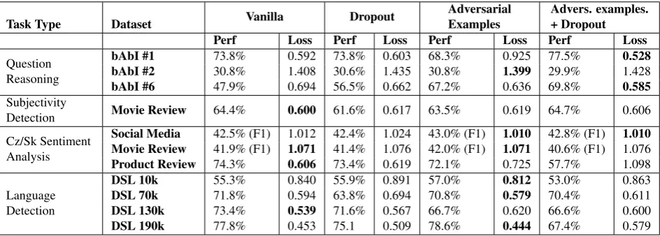
During the evaluation, we focus on the testing loss improve-ment in comparison with the original vanilla model. We do not aim to compare our results with state-of-the-art results that usually employ additional (possibly hand-crafted) tech-niques during the training. All our results are presented in Table 1.

At least two models differing in the number of parameters (referred to as the big and small models) were trained for each experiment. Throughout our experiments, the smaller models tend to underfit the given task and the use of ad-versarial examples had no effect. In contrast, the bigger models tend to overfit massively which made regulariza-tion methods such as dropout or the adversarial examples effective. In the following text, we report only the results of the big models.

In addition, we experimented with both LSTM and GRU recurrent cells which, to our knowledge, did not affect the overall model performance. The presented results repre-sent the models which employ bidirectional GRU recurrent cells.

All experiments compare four models (see Table 1): 1. the vanilla model (without any regularization), 2. the same model trained with dropout (embedding

layer, MLP hidden layer),

3. the same model trained with adversarial examples, 4. the same model trained with both adversarial

exam-ples and dropout.

We start by evaluating the bAbI datasets, namely bAbI #1, #2 and #6. In all bAbI experiments we use a model which employs embeddings of dimension 100, which we experi-mentally discovered to be sufficient (increasing the dimen-sion does not affect training). The GRU dimendimen-sion is set to 400 and MLP hidden layer dimension is set to 512. Focusing mainly on the test performance which represents the actual model generalization, we observe that the em-ployment of the adversarial perturbations together with dropout provides approximately 22% accuracy improve-ment5 _{in the case of bAbI #6. On the contrary, the} em-ployment of dropout provides only approximately 10% ac-curacy gain.

In contrast with the previous experiment, the employment of the adversarial examples damaged the model perfor-mance in the case of bAbI #1. However, the dataset ac-curacy benefited from using both adversarial training and dropout by approximately 4%.

For both experiments, we tested the testing loss differ-ence between the vanilla model and the one employing the adversarial training. All measurements indicate that the testing losses significantly differ at the significance level

α = 0.05, which was set in advance (p-values0.003and 0.001, respectively).

Both datasets outperformed the baselines set by Weston et al. (2015) when evaluating the weakly supervised cases. The final selected bAbI dataset (#2) which represents more

Task Type Dataset Vanilla Dropout

Adversarial Examples

Advers. examples. + Dropout Perf Loss Perf Loss Perf Loss Perf Loss

Question Reasoning

bAbI #1 73.8% 0.592 73.8% 0.603 68.3% 0.925 77.5% 0.528 bAbI #2 30.8% 1.408 30.6% 1.435 30.8% 1.399 29.9% 1.428

bAbI #6 47.9% 0.694 56.5% 0.662 67.2% 0.636 69.8% 0.585

Subjectivity

Detection Movie Review 64.4% 0.600 61.6% 0.617 63.5% 0.619 64.7% 0.606 Cz/Sk Sentiment

Analysis

Social Media 42.5% (F1) 1.012 42.4% 1.024 43.0% (F1) 1.010 42.8% (F1) 1.010 Movie Review 41.9% (F1) 1.071 41.4% 1.076 42.0% (F1) 1.071 40.6% (F1) 1.076

Product Review 74.3% 0.606 73.4% 0.619 72.1% 0.725 57.7% 1.098

Language Detection

DSL 10k 55.3% 0.840 55.9% 0.891 57.0% 0.812 53.0% 0.863

DSL 70k 71.8% 0.594 63.8% 0.694 70.8% 0.579 70.4% 0.611

DSL 130k 73.4% 0.539 71.6% 0.567 66.7% 0.620 66.6% 0.600

DSL 190k 77.8% 0.453 75.1 0.509 78.6% 0.444 67.4% 0.579

Table 1: The first and second columns describe the task type and the dataset name, respectively. The final four columns demonstrate the testing accuracies or F1-scores and the mean testing losses. The bold formatting indicates the loss which is the best among the dataset experiment.

challenging questions has not significantly benefited from the employment of the adversarial examples.

The next evaluated dataset is the Movie Review dataset for subjectivity detection. We use a model which employs embeddings of dimension 200; the GRU dimension is set to 200 and MLP hidden layer dimension is set to 256. We observe that employing both adversarial examples and dropout during training stabilizes it. Approximately 0.3% increase in accuracy is achieved, however, the testing loss is significantly smaller (p-value 0.039) than the testing loss yielded by the model with only dropout. We suggest that the model is more confident of its responses.

Then, we evaluated the three Czech/Slovak sentiment anal-ysis datasets. We used all four classes (positive, negative, neutral, bi-polar) and trained models using the their pho-netic transcriptions. We have experimented also with stem-ming instead of phonetic transcriptions, however, the per-formance was poor and all models tended to overfit in early epochs.

The Social Media dataset benefited from the adversarial training by 0.05% increase in F1-score and the testing loss significantly decreases either with or without using dropout (p-values 0.009 and 0.026, respectively). We observe sim-ilar gain in F1-score (+0.15%) in the case of omitting the bi-polar class. For these experiments we employ embed-dings of dimension 200; the GRU dimension is set to 400 and MLP hidden layer dimension is set to 512.

The sentiment analysis dataset (Movie Review) has not sig-nificantly benefited from the adversarial examples. The performance of the final sentiment analysis dataset (Product Review) surprisingly decreased in all our exper-iments when using the adversarial examples even though it is similar to the previous two datasets. The main difference is the size of the dataset as the Product Reviews contains much more training examples. We experiment also with character-level models (presented in Table 1) for which we employ embeddings of dimension 15; the GRU dimension is set to 400 and MLP hidden layer dimension is set to 512. The last dataset that we evaluate is the Discriminating be-tween Similar Language (DSL) dataset which we attempt to model also on a character level. We evaluated this dataset

multiple-times with various training set size limits (10, 70, 130 and 170 thousand of examples).

In all DSL experiments we use a model which employs em-beddings of dimension 20. The GRU dimension is set to 200 and MLP hidden layer dimension is set to 256. The results of the experiments which were trained us-ing the smallest trainus-ing set and regularized by adversar-ial examples indicate that the use of adversaradversar-ial examples significantly improves the training loss (relative drop of 4%). At the same time, the model accuracy is improved as well. Contrary to this observation, the experiments with the larger training sets have not benefited in accuracy when employing adversarial examples either with or with-out dropwith-out. Nevertheless, the average testing losses have (except the 130k training set) significantly decreased. We conclude that the greater the training set is, the smaller im-pact the adversarial training makes.

6.

Discussion

The conducted experiments lead us to the following claims. Firstly, we observe that the employment of adversarial ex-amples improves the model loss on majority of datasets of our collection.6

We conclude that the models whose capacity is sufficient so that they overfit the training data (the number of their parameters is large) can benefit from using adversarial ex-amples. In these cases, we claim that employing adversarial examples during training acts as a regularization technique. Furthermore, our preliminary hypotheses on the trends be-tween the dataset characteristics and the effect of using the adversarial examples are as follows. Note that a wider col-lection of datasets would be required to make our proposi-tions more credible.

English datasets exhibited better performance from the ad-versarial examples than the Czech or Slovak ones. We hy-pothesize that this effect might be caused by the fact that the Slavic languages feature a more complex morphology

6

and a greater number of distinct words (tokens). Neverthe-less, even though strict stemming was employed, we did not achieve such performance improvement compared to the one we have observed in other English datasets. Furthermore, we claim that the networks trained on artifi-cial data (such as bAbI tasks (Weston et al., 2015)) with a rather small number of distinct tokens are more likely to bevulnerableto adversarial examples and their use during training prevents the model from overfitting particularly ef-ficiently.

Based on our experiments, we observe that the impact of the studied technique decreases as the size of the training dataset increases. We conclude that this phenomenon sup-ports the hypothesis that adversarial training serves as a reg-ularization technique, which is usually less effective in case more training data is available.

We provide novel evidence that the adversarial perturbation of character embeddings can also lead to performance im-provement when used in the process of training character-level models.

7.

Conclusion

This paper focuses on employing adversarial examples dur-ing traindur-ing of deep recurrent neural networks. The contri-bution of this paper is threefold.

Firstly, we compiled a collection of eight datasets for which a unified stream interface was created. The datasets were chosen in order to represent a distinct set of characteristics which were chosen in advance.

Secondly, the employment of adversarial examples during the network training was evaluated in various settings. We focused on embeddings which are randomly initialized at the beginning of the training.

Finally, we have proposed several hypotheses about rela-tions between the dataset characteristics and the effect of model training when using adversarial examples. In some cases, we outperformed the baselines provided by the au-thors of the dataset publications.

We conclude that the adversarial training can function as a regularization for RNNs processing natural text. This is a direct extension of the work of Miyato et al. (2016a) who have experimented with pretrained embeddings.

7.1.

Future Work

We consider the following possible research directions in our future work regarding the adversarial examples. Firstly, additional datasets might be evaluated in order to provide more detailed study. In particular, tasks such as machine translation, which do not aim to classify the in-put, could be studied. For this purpose, supplementary ar-chitectures such as sequence-to-sequence modelsshall be evaluated.

Secondly, our further research will focus on the embedding structure analysis, primarily on the changes caused by em-ploying the adversarial examples. Even though we have not been able to prove a significant change in their struc-ture yet, we hope the interpretation of the embedding dif-ferences might be found. In addition, we will study the stability of training when using adversarial examples.

Furthermore, supplementary techniques for adversarial ex-ample creation will be analyzed, notably Generative Ad-versarial Networks (Goodfellow et al., 2014a). Another approach could employ genetic algorithms for embedding perturbations.

Finally, additional types of machine learning, such as (deep) reinforcement learning (RL) could be examined. Fo-cusing on NLP, the end-to-end neural dialogue systems are suitable for further analysis.

8.

Acknowledgements

The research described herein has been supported by the Grant No. DG16P02B048 of the Ministry of Culture of the Czech Republic. Data has been used from and stored into the LINDAT/CLARIN repository, a large research infras-tructure supported by the Ministry of Education, Youth and Sports of the Czech Republic under projects LM2015071 and CZ.02.1.01/0.0/0.0/16 013/0001781.

Access to computing and storage facilities owned by parties and projects contributing to the National Grid Infrastructure MetaCentrum provided under the programme ”Projects of Large Research, Development, and Innovations Infrastruc-tures” (CESNET LM2015042), is greatly appreciated.

9.

Bibliographical References

Amodei, D., Ananthanarayanan, S., Anubhai, R., Bai, J., Battenberg, E., Case, C., Casper, J., Catanzaro, B., Cheng, Q., Chen, G., et al. (2016). Deep speech 2: End-to-end Speech Recognition in English and Mandarin. In International Conference on Machine Learning, pages 173–182.

Ba, J. L., Kiros, J. R., and Hinton, G. E. (2016). Layer Normalization. arXiv preprint arXiv:1607.06450. Bishop, C. M. (1995). Training with noise is equivalent to

tikhonov regularization. Neural computation, 7(1):108– 116.

Caswell, I., Nie, A., and Sen, O. (2016). Exploring Ad-versarial Learning on Neural Network Models for Text Classification. Standford NLP Project.

Cho, K., Van Merri¨enboer, B., Gulcehre, C., Bahdanau, D., Bougares, F., Schwenk, H., and Bengio, Y. (2014). Learning Phrase Representations Using RNN Encoder-Decoder for Statistical Machine Translation.Conference on Empirical Methods in Natural Language Processing. Collobert, R. and Weston, J. (2008). A Unified Archi-tecture for Natural Language Processing: Deep Neural Networks with Multitask Learning. In Proceedings of the 25th international conference on Machine learning, pages 160–167. ACM.

Fawzi, A., Moosavi-Dezfooli, S.-M., and Frossard, P. (2016). Robustness of Classifiers: From Adversarial to Random Noise. InAdvances in Neural Information Pro-cessing Systems, pages 1624–1632.

Goodfellow, I. J., Shlens, J., and Szegedy, C. (2014b). Ex-plaining and Harnessing Adversarial Examples. Interna-tional Conference on Learning Representations. Grandvalet, Y., Canu, S., and Boucheron, S. (1997). Noise

injection: Theoretical prospects. Neural Computation, 9(5):1093–1108.

Habernal, I., Pt´aˇcek, T., and Steinberger, J. (2013). Senti-ment Analysis in Czech Social Media Using Supervised Machine Learning. InProceedings of the 4th workshop on computational approaches to subjectivity, sentiment and social media analysis, pages 65–74.

Hinton, G. E., Srivastava, N., Krizhevsky, A., Sutskever, I., and Salakhutdinov, R. R. (2012). Improving Neural Net-works by Preventing Co-adaptation of Feature Detectors. Journal of Machine Learning Research.

Hochreiter, S. and Schmidhuber, J. (1997). Long Short-Term Memory. Neural computation, 9(8):1735–1780. Ioffe, S. and Szegedy, C. (2015). Batch Normalization:

Accelerating Deep Network Training by Reducing Inter-nal Covariate Shift. ICML.

Ioffe, S. (2017). Batch renormalization: Towards reduc-ing minibatch dependence in batch-normalized models. arXiv preprint arXiv:1702.03275.

James, G., Witten, D., Hastie, T., and Tibshirani, R. (2013). An Introduction to Statistical Learning, vol-ume 6. Springer.

Jia, R. and Liang, P. (2017). Adversarial examples for eval-uating reading comprehension systems. InProceedings of the 2017 Conference on Empirical Methods in Natural Language Processing, pages 2011–2021.

Kingma, D. and Ba, J. (2014). Adam: A Method for Stochastic Optimization. arXiv preprint arXiv:1412.6980.

Klambauer, G., Unterthiner, T., Mayr, A., and Hochre-iter, S. (2017). Self-normalizing neural networks.arXiv preprint arXiv:1706.02515.

Lu, J., Issaranon, T., and Forsyth, D. (2017). Safetynet: Detecting and Rejecting Adversarial Examples Robustly. arXiv preprint arXiv:1704.00103.

Maas, A. L., Daly, R. E., Pham, P. T., Huang, D., Ng, A. Y., and Potts, C. (2011). Learning Word Vectors for Sentiment Analysis. InProceedings of the 49th Annual Meeting of the Association for Computational Linguis-tics: Human Language Technologies-Volume 1, pages 142–150. Association for Computational Linguistics. Matsuoka, K. (1992). Noise injection into inputs in

back-propagation learning. IEEE Transactions on Systems, Man, and Cybernetics, 22(3):436–440.

Mikolov, T., Chen, K., Corrado, G., and Dean, J. (2013). Efficient Estimation of Word Representations in Vector Space. ICLR Workshop.

Miyato, T., Dai, A. M., and Goodfellow, I. (2016a). Adver-sarial Training Methods for Semi-Supervised Text Clas-sification.arXiv preprint arXiv:1605.07725.

Miyato, T., Dai, A. M., and Goodfellow, I. (2016b). Virtual Adversarial Training for Semi-Supervised Text Classifi-cation. arXiv preprint arXiv:1605.07725.

Moosavi-Dezfooli, S.-M., Fawzi, A., Fawzi, O., and

Frossard, P. (2016a). Universal Adversarial Perturba-tions.arXiv preprint arXiv:1610.08401.

Moosavi-Dezfooli, S.-M., Fawzi, A., and Frossard, P. (2016b). Deepfool: A Simple and Accurate Method to Fool Deep Neural Networks. InProceedings of the IEEE Conference on Computer Vision and Pattern Recogni-tion, pages 2574–2582.

Nguyen, A., Yosinski, J., and Clune, J. (2015). Deep Neu-ral Networks Are Easily Fooled: High Confidence Pre-dictions for Unrecognizable Images. InProceedings of the IEEE Conference on Computer Vision and Pattern Recognition, pages 427–436.

Pang, B. and Lee, L. (2004). A Sentimental Education: Sentiment Analysis Using Subjectivity Summarization Based on Minimum Cuts. In Proceedings of the 42nd annual meeting on Association for Computational guistics, page 271. Association for Computational Lin-guistics.

Papernot, N., McDaniel, P., Goodfellow, I., Jha, S., Celik, Z. B., and Swami, A. (2016a). Practical Black-box At-tacks Against Deep Learning Systems Using Adversarial Examples.arXiv preprint arXiv:1602.02697.

Papernot, N., McDaniel, P., Jha, S., Fredrikson, M., Celik, Z. B., and Swami, A. (2016b). The Limitations of Deep Learning in Adversarial Settings. In Security and Pri-vacy (EuroS&P), 2016 IEEE European Symposium on, pages 372–387. IEEE.

Rajpurkar, P., Zhang, J., Lopyrev, K., and Liang, P. (2016). Squad: 100,000+ questions for machine comprehension of text. arXiv preprint arXiv:1606.05250.

Salimans, T. and Kingma, D. P. (2016). Weight normaliza-tion: A simple reparameterization to accelerate training of deep neural networks. InAdvances in Neural Infor-mation Processing Systems, pages 901–909.

Simard, P. Y., Steinkraus, D., Platt, J. C., et al. (2003). Best practices for convolutional neural networks applied to visual document analysis. InICDAR, volume 3, pages 958–962.

Sukhbaatar, S., Weston, J., Fergus, R., et al. (2015). End-to-end Memory Networks. InAdvances in neural infor-mation processing systems, pages 2440–2448.

Szegedy, C., Zaremba, W., Sutskever, I., Bruna, J., Erhan, D., Goodfellow, I., and Fergus, R. (2013). Intriguing Properties of Neural Networks. International Confer-ence on Learning Representations.

Vidnerov´a, P. and Neruda, R. (2016). Evolutionary Gen-eration of Adversarial Examples for Deep and Shal-low Machine Learning Models. In Proceedings of the The 3rd Multidisciplinary International Social Networks Conference on SocialInformatics 2016, Data Science 2016, page 43. ACM.

Wang, Y., Skerry-Ryan, R., Stanton, D., Wu, Y., Weiss, R. J., Jaitly, N., Yang, Z., Xiao, Y., Chen, Z., Bengio, S., et al. (2017). TACOTRON: Towardss End-to-end Speech Synthesis.arXiv preprint arXiv:1703.10135. Weston, J., Bordes, A., Chopra, S., Rush, A. M., van

Yin, J., Jiang, X., Lu, Z., Shang, L., Li, H., and Li, X. (2015). Neural Generative Question Answering. arXiv preprint arXiv:1512.01337.