Exploratory Neural Relation Classification for Domain Knowledge Acquisition

Proceedings of the 27th International Conference on Computational Linguistics, pages 2265–2276 2265

Exploratory Neural Relation Classification for Domain Knowledge

Acquisition

Yan Fan, Chengyu Wang, Xiaofeng He∗

School of Computer Science and Software Engineering, East China Normal University, Shanghai, China

{eileen940531,chywang2013}@gmail.com, [email protected]

Abstract

The state-of-the-art methods for relation classification are primarily based on deep neural net-works. This supervised learning method suffers from not only limited training data, but also the large number of low-frequency relations in specific domains. In this paper, we propose an ex-ploratory relation classification method for domain knowledge harvesting. The goal is to learn a classifier on pre-defined relations while discovering new relations expressed in texts. A dynami-cally structured neural network is introduced to classify entity pairs to a continuously expanded relation set. We further propose the similarity sensitive Chinese restaurant process to discover new relations. Experiments conducted on a large corpus show that new relations are discovered with high precision and recall, illustrating the effectiveness of our method.

Title and Abstract in Chinese

基于领_域知_{识获取的探索}式_神经网_络关_系分类

近几_年来，关_{系分类任务主要利}用_神经网_络模_型来自_动学习复_杂的特征_。然而这_类监督

式_学习方法_的局_限性_在于，首先_它需要大量_{训练数据，}其次特_定领_域存在长尾_的低频关

系无法_被有效地预_{定义。在本论文中，}我_们提出_了基于领_域知_{识获取的探索}式关_系分类

任务。它的目标在于学习预_定义关_{系的分类器，同时从文本中发现新的语义}关_系。我_们

提出_了一个动态_{结构的神经}网_{络，它可以对持续}扩充_的关_系集进_行分类。我_们进_一步_提

出_{了相似度敏感的中餐馆}过程算法_，用_于发现新关_系。基于大_{语料库上的实}验_证明了该

神经网_{络的分类效果，同时新发现的}关_系也有较高_的准_{确率和召回率。}

1 Introduction

Relation classification assigns semantic relation labels to entity pairs in texts. Besides traditional feature-based (Kambhatla, 2004) and kernel-feature-based (Bunescu and Mooney, 2005) approaches, neural networks (NNs) are introduced to harvest relational facts in recent years. Classical architectures include convolu-tional neural networks (CNNs) (Zeng et al., 2014), recurrent neural networks (RNNs) (Xu et al., 2015), etc. However, above methods are still insufficient for domain knowledge acquisition due to two chal-lenges: (i) most domain entities rarely occur in the corpus, hence pattern-based methods easily suffer from the feature sparsity problem; (ii) a domain knowledge graph tends to be incomplete w.r.t. relation labels and facts (Fan et al., 2017). As a result, unlabeled entity pairs are likely to be wrongly forced into existing relation labels by distant supervision approaches, instead of their true, unknown labels.

In this paper we propose a method, Exploratory Relation Classification (ERC), to populate domain knowledge graphs automatically. The goal of ERC is to not only classify entity pairs into a finite set of pre-defined relations, but also simultaneously discover previously unseen relation types and their respective instances from plain texts with high confidence. The resulting numbers of relation types and facts in the domain knowledge graph grow continuously.

∗

Corresponding author.

To solve ERC problem, we propose a Dynamic Structured Neural Network (DSNN). In the network, the convolutional and recurrent network units are employed to model local information such as syntactic and lexical features from the sentence level. For the context sparsity problem (Challenge (i)) an embed-ding layer is introduced to encode corpus-level semantic features of domain entities. The output classes of DSNN can be automatically expanded during the iterative training process, in order to classify entity pairs to both known and newly discovered relations. To explore new relations and corresponding in-stances, we introduce the similarity sensitive Chinese restaurant process (ssCRP) to generate clusters of entity pairs from unlabeled data that can not be classified into any known relations (Challenge (ii)). We can see that the DSNN only takes the training data of known relations directly derived from a domain knowledge graph without requiring any training data for new relations. Therefore, our approach is a very weakly supervised one with minimal human intervention.

The rest of the paper is organized as follows. Section 2 summarizes the related work and discusses relations between existing methods and ours. The detailed approach is introduced in Section 3, Section 4 and Section 5, with experiments presented in Section 6. Finally, we conclude this paper in Section 7.

2 Related Work and Discussion

In NLP research, feature-based (Kambhatla, 2004) and kernel-based (Bunescu and Mooney, 2005) meth-ods have been proposed to utilize lexical, syntactic and semantic features for relation classification. In recent years, neural network based approaches are introduced to improve the performance. Word embed-dings of entities are frequently used as inputs, instead of one-hot representations (Mikolov et al., 2013; Pennington et al., 2014). As shown in (Wang and He, 2016; Wang et al., 2017), word embeddings can be used for relation prediction. For neural network architectures, CNNs are capable of learning consecutive contexts of entities as local lexical features (Zeng et al., 2014; Vu et al., 2016), while RNNs exploit syn-tactic features by modeling long-term dependencies of sentences via memory units. The model of Long Short Term Memories (LSTMs) (Hochreiter and Schmidhuber, 1997) is an effective variant of RNNs to encode the shortest dependency path (SDP) between entity pairs (Xu et al., 2015; Shwartz et al., 2016). More recent work focuses on the design of integrated architecture, combining both CNNs and RNNs. Cai et al. (2016) propose a bidirectional recurrent CNN to model the directional information along the SDP forwards and backwards. The integrated neural network proposed by Raj et al. (2017) also exper-iments with attention-based pooling strategy for biomedical texts. Our model provides a more intuitive representation by feature concatenation instead of network layering, enabling the adaption of dynamic changes as new relations are discovered in iterations.

For relation discovery, one way is to formulate the task as open relation extraction (OpenRE) (Banko et al., 2007). Typical OpenRE systems include TextRunner (Banko et al., 2007), WOE (Wu and Weld, 2007), ReVerb (Etzioni et al., 2011), etc. Unlike approaches confined to a fixed set of pdefined re-lations, these systems explore relations in a more general way. Contrary to the fact that the contexts for domain knowledge are sparse, the underlying idea of OpenRE is to identify phrases from sentences that are able to indicate unknown relations based on data redundancy. Therefore, OpenRE methods are not suitable for domain-specific knowledge harvesting within a limited text corpus. Similarly, Riedel et al. (2013) learn universal schemas by matrix factorization without pre-defined relations. An alterna-tive way is to use clustering algorithms. Compared to standard clustering algorithms (e.g., KMeans), non-parametric Bayesian models (Rasmussen, 1999) are more suitable in our scenario, because they can automatically learn the number of clusters. Studies afterwards exploit data features for spatial and temporal data, such as distance dependent CRP (ddCRP) (Blei and Frazier, 2010), etc.

methods applied on such corpus will introduce plenty of small classes, which are in fact noises and thus meaningless. In contrast, our ssCRP-based approach works more effectively since we only discover one large class with confident instances in each iteration. Hence such noises in the data will not be forced to generate small classes and are automatically discarded when the last iteration stops.

3 Dynamic Structured Neural Network for ERC

In this section, we present the definition of the task ERC and a high level introduction of the DSNN approach.

3.1 Task Definition

Before introducing the training process of DSNN, we first provide some preliminaries. Denote entity pairs asXl ={(e1, e2)}with corresponding labelsYl, and unlabeled entity pairs asXu ={(e1, e2)}.

Exploratory Relation Classification (ERC) task is defined as follows:

Definition 1. Given labeled data(Xl, Yl)and unlabeled dataXu, the goal of ERC is to train a model to predict the relations for entity pairs inXuwithK+noutput labels, whereKdenotes the number of pre-defined relations inYl, andnis the number of newly discovered relations which is unknown.

3.2 An Overview of DSNN

Algorithm 1 shows the iterative training process of DSNN. In each iteration, the algorithm tries to detect a new relation from unlabeled data based on ssCRP, and expands the neural network structure to perform relation classification over existing and new relations. Briefly, it consists of three modules: base neural network training1, relation discovery and relation prediction.

Algorithm 1DSNN Training Process

Input: Entity pairsXland their labelsYl, unlabeled entity pairsXu, pre-defined relation setRold={r1, . . . , rK}

Output: New relation setRnew={rK+1, . . . , rK+n}, populated labeled entity pairsXland their labelsYl

1: InitializeRnew =Rold, t= 1

2: whileno new relations can be discovereddo 3: // Base neural network training

4: Train base neural networkN NtwithXl_andYl 5: // Relation discovery

6: Generate candidate clusters{C1, . . . , Cm}=ssCRP(Xu, Xl)

7: C∗=PickTheBestCluster(C1, . . . , Cm)

8: r∗=MapToRelation(C∗) 9: ifr∗∈/Roldthen 10: Rnew=Rnew∪ {r∗_} 11: end if

12: Label all entity pairs inC∗with relationr∗to beY∗ 13: Xl=Xl∪C∗,Yl=Yl∪Y∗,Xu=Xu\C∗ 14: // Relation prediction

15: for each(e1, e2)inXudo

16: Pr(r|e1, e2, N Nt) =PredictRelDistribution(e1, e2, Rold, N Nt)

17: ifNotNearUniform(Pr(r|e1, e2, N Nt))then

18: Label(e1, e2)with relation argmaxr∗Pr(r|e1, e2, N Nt)to beY∗

19: Xl_=Xl_{∪ {(e}

1, e2)},Yl=Yl∪Y∗,Xu=Xu\{(e1, e2)}

20: end if 21: end for

22: Rold=Rnew,t=t+ 1 23: end while

24: return Rnew,Xl_,Yl

In each iterationt, the first step is to train base neural network N Ntwith training data Xl andYl.

Note that in the first iteration, model N Nt is trained fully supervised. Whent > 1, N Nt is trained

semi-supervisedly, utilizing both labeled training data and new relations discovered in previoust−1

iterations.

E D H C > O (,,

C

-A *) >

> > E O C

E O D

C OC

LSTM LSTM LSTM

- B

Input

Sentence LSTM network

Lookup table

Convolution and Pooling

Syntactic context Lexical context Semantic context Word embedding

Part-of-speech tag Dependency relation Relational direction

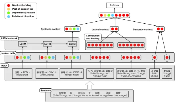
Figure 1: The architecture of the base neural network withk=2.

AfterN Ntis trained, ssCRP is employed to generatemclusters fromXu (i.e.,C1, . . . , Cm), where

each cluster represents the collection of entity pairs that are most likely to share the same underlying relation. We select the “best” clusterC∗fromC1, . . . , Cmbased on the size and intra-cluster similarity,

and map it to the relationr∗. r∗ could either be one of the pre-defined relations, or a newly discovered relation. Either way, we updateXlandYlwithC∗labeled asr∗, and remove them fromXu.

For unlabeled entity pairs(e1, e2) ∈ Xu, we use modelN Ntto predict the probability distribution Pr(r|e1, e2, N Nt) over all possible relations. If the distribution is not “near uniform”, the model is

confident to predict the relationr∗ = argmaxPr(r|e1, e2, N Nt). Hence,(e1, e2)will be labeled asr∗

and added to labeled data (i.e.,XlandYl). Here, we only add unlabeled data with confident predictions to the training set, in order to avoid error propagation in a semi-supervised learning environment.

After the execution of the above three modules in one iteration, if a new relation is found with its seed relation instances (i.e., entity pairs), the structure of the neural network retrained in the next iteration will be adjusted dynamically with parameters updated.

4 The Architecture of the Base Neural Network

Base neural network takes texts with annotated entity pairs as input and classify them to a fixed relation set. It learns representation of texts by exploiting the following three contexts: (i) syntactic contexts; (ii) lexical contexts; and (iii) global semantic contexts. The overall architecture is illustrated in Fig. 1.

Syntactic contexts. Previous work exploits the shortest dependency path (SDP) (Bunescu and Mooney, 2005) to capture predicate-argument sequences (Cai et al., 2016; Xu et al., 2015; Shwartz et al., 2016). However, SDP can not handle the dependency relation properly betweene1 ande2due to

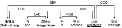
the lack of the associated predicate. Consider the example in Fig. 2. Entities “张智霖 (Zhilin Zhang)” and “袁咏仪(Yongyi Yuan)” are in the coordinate dependency relation via a direct arc. Thus, the SDP between two entities is “张智霖(Zhilin Zhang)→_袁咏仪 (Yongyi Yuan)”, which contains not much useful information. In this paper, we design a structure to capture the root verb along the dependency path, namely root augmented dependency path (RADP):

Definition 2. An RADP is the combination of two subpaths derived from the dependency graph, one from

e1to the root verb, and the other one from the root toe2.

Here, the RADP is “注册(registered)→张_智霖(Zhilin Zhang)→_袁咏仪(Yongyi Yuan) ”. Com-pared to SDP, it includes the extra root verb “注册 (registered)”, a crucial complement indicating the relation “配偶(spouse)” holds between two entities.

Zhilin Zhang and Yongyi Yuan in America registered marriage SBV

LAD

COO ADV

POB

COO

Figure 2: An example of the dependency graph.

where~vword,~vpos,~vrel,~vdirare the embeddings of the word, POS tag, dependency relation and relational

direction, respectively. [·]is the concatenation of embeddings. These embeddings are initialized as one-hot vectors except for~vword, pre-trained on a large corpus.

We employ an LSTM network to handle the long-term dependencies. For an RADP with sequence

w1, . . . , wj, the corresponding embeddings~vsyn1, . . . , ~vsynj are fed into an LSTM network. The output vector~vlstmis the context vector modeling the syntactic features of the whole sequence.

Lexical contexts. Specific patterns around target entities can imply semantic relations between entity pairs (Hearst, 1992). Similar to previous research (Zeng et al., 2014; Vu et al., 2016), given a window size

k, we define the lexical context of an annotated entity askwords ahead andkwords following. Formally, the lexical context vector~vconis represented as follows:~vcon = [~vwi−k, . . . , ~vwi−1, ~vei, ~vwi+1, . . . , ~vwi+k]

where~veiand~vwj are embeddings of entity and context word at indexiandj.

For entities e1 and e2 in the pair,~vcone₁ and~vcone₂ are fed into CNN units, respectively. After a

convolutional layer and a max pooling layer, the resulting vectors are concatenated as~vcnn.

Semantic contexts. The context-sparsity problem of domain knowledge motivates us to explore se-mantic contexts in the global corpus, instead of being limited to local features. Based on the distributional hypothesis, we train a Skip-gram model (Mikolov et al., 2013) to learn the distributional representations of words in a large corpus. For entity paire1ande2, the embeddings~ve1and~ve2are further concatenated to build the final representation of semantic contexts:~vemb= [~ve1, ~ve2].

Prediction. The final context representation for prediction is the concatenation of three resulting vectors~vf = [~vlstm, ~vcnn, ~vemb]. Then we apply asoftmaxlayer on~vf to predict the class distributiony:

~

y=softmax(W ·~vf+b)whereW is the transformation matrix andbis the bias vector. The prediction

of base neural network is the relation whose probability is maximal in~y.

5 Relation Discovery

To expand the output layer of base neural network, a clustering algorithm ssCRP is proposed to explore new relations from unlabeled data. In this part, we first introduce how the network expands, and briefly cover the basics of CRP, followed by the algorithm ssCRP in detail.

5.1 Network Expansion

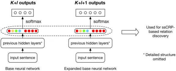
After training base neural network, we take its final hidden layer as the representation for each entity pair, since it contains all high-level context features. The representations used as the input of ssCRP should be close to each other in the embedding space, if the same relation holds for these pairs.

In iterationt, ssCRP and the table selection process (to be discussed later) generate a clusterC∗ from unlabeled data. Letr∗ be the mapping relation that entity pairs inC∗ hold, {r1, . . . , rK+l}be theK

pre-defined relations andlnew relations discovered int−1iterations. If r∗ ∈ {/ r1, . . . , rK+l}, a new

relation is found and base neural network trained in the next iterationt+ 1expands its output layer with an extra class; otherwise, it remains the same with K+l output classes. Fig 3 shows the base neural network and its expansion network.

5.2 Similarity Sensitive Chinese Restaurant Process

Preliminaries. The Chinese restaurant process (CRP) is a stochastic process, which groups customers into random tables where they sit (Aldous, 1985). AssumeNp denotes the number of customers sitting

previous hidden layers*

K+l outputs K+l+1 outputs

softmax

Used for ssCRP-based relation

discovery

input sentence * Detailed structure _omitted

Base neural network

previous hidden layers*

softmax

input sentence

Expanded base neural network

Figure 3: Base neural network and the expanded network.

table assignment for other customers. The distribution over table assignments is as follows:

Pr(zi=p|~z−i, α)∝ (

Np ifp≤K

α ifp=K+ 1 (1)

whereαis a scaling parameter andKis the number of occupied tables.

ssCRP.Although CRP can be applied for clustering in a non-parametric Bayesian fashion, it does not consider the similarity of relation instances. We observe that some extensions of CRP (e.g., ddCRP (Blei and Frazier, 2010)) leverage the distances between data points but they do not consider the iterative clus-ter generation process with pre-defined clusclus-ters. In this paper, we propose a similarity-based clusclus-tering algorithm especially designed for ERC, called similarity sensitive Chinese restaurant process (ssCRP).

In ssCRP, we turn the problem of table assignment into customer assignment. Unlike the CRP and ddCRP, we accommodate labeled data by initializing tables withK pre-defined classes. Customerihas the choice of sitting next to any customerjbased on similarity, which leads to three cases: (i)ijoins the table wherejsits; (ii)iand an upcomingjgenerates a new table2; and (iii)isits at an empty table alone. Case (i) is specifically introduced for task ERC due to the initialization of existing tables. Each table in case (i) can be represented as a virtual customer averaged from all its seated customers.

Denote η = {S, N, α, β}as the set of hyperparameters, where S is a similarity matrix between all customers,N = (N1,· · · , NK)is the size vector of existingKtables,αis the scaling parameter andβ

is a parameter balancing the weight of table size. The distribution of customer assignmentciis:

Pr(ci =j|η)∝   

 

α ifjis customeriitself

g(sij) ifjis an upcoming customer

g(sij)(1 +βlgNp) ifjis averaged from tablep

(2)

wheregis a function modeling the cosine similaritysij between customeriandj. We design a

magni-fying functiong(sij) = −1/lnsij wheresij >0, to increase the dissimilarity of inputs. The first two

cases in Eq. (2) are derived from CRP. The third case gives existing tables additional weights to avoid generating too many small clusters. An alternative measuring system is to use the distance function

dij = 1−sij and to apply different non-increasing functions to mediate the distances between

cus-tomers. Given a parametera, typical decay functions like window decayf(d) = 1[d < a], exponential decayf(d) = exp(d/a)and logistic decay f(d) = exp(−d+a)/(1 +exp(−d+a))are provided as alternatives (Blei and Frazier, 2010).

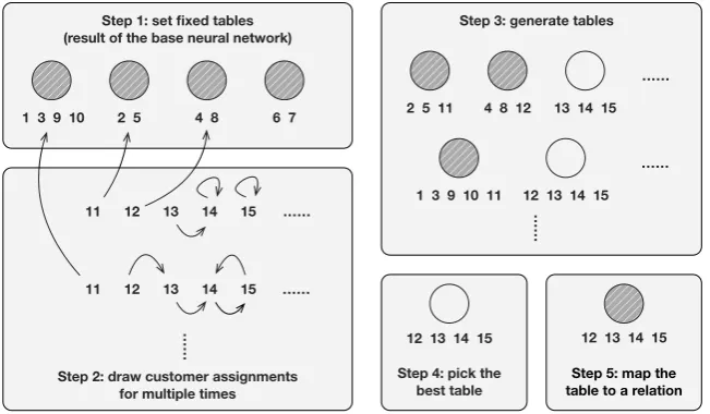
ssCRP-based relation discovery. The overall sampling and table selection process is illustrated in Fig. 4. In Step 1, we initialize fixed tables with classification results of labeled data. In Step 2, ssCRP draws customer assignments based on Gibbs sampling. DenoteCpas the collection of entity pairs w.r.t

tablep. Given the hyperparameter setη, the likelihood function of tablepdenoted byCp is calculated

as follows:Pr(Cp |η) = Q|Cp|

i=1 Pr(c p

i |η)wherec p

i represents the customer assignment that customeri

sits at tablep.

1 3 9 10 2 5 4 8 6 7 Step 1: set fixed tables (result of the base neural network)

11 12 13 15

11 12 13 14 15

14

Step 2: draw customer assignments for multiple times

……

……

2 5 11 4 8 12 13 14 15

……

1 3 9 10 11 12 13 14 15

……

……

……

Step 3: generate tables

12 13 14 15

Step 4: pick the best table

12 13 14 15

Step 5: map the table to a relation

Figure 4: Relation discovery based on ssCRP. Circles with shadow are existing relations, while plain circles are new tables surrounded with customers representing entity pairs.

1 2 3 4 5 6 7

(a) i links to itself

1 2 3 4 6 7

(b) i links to a new table where j sits

1 2 3 4 5 6 7

(c) i links to an existing table p where j sits

1 2 3 6 7

(d) i joins two new tables

p and q

1 2 3 6 7

(e) i joins an existing table

p and a new table q

5 4 5 4 5

Figure 5: Five cases of customer assignment with i = 4 based on Gibbs sampling. Grey boxes are existing tables while white ones are generated new tables.

Given the rest of customer assignments c−i, customer assignmentci can be divided into five cases

(Blei and Frazier, 2010), generated by Gibbs sampling as Fig. 5 shows:

Pr(ci =j|c−i, η)∝                  α (a)

g(sij) (b)

g(sij)(1 +βlgNp) (c)

g(sij)_{Pr(Cp|η) Pr(Cq|η)}Pr(Cp∪Cq|η) (d)

g(sij)(1 +βlgNp)_{Pr(Cp|η) Pr(Cq|η)}Pr(Cp∪Cq|η) (e)

(3)

After this process, all customers are connected together with direct links from one to another or self-loops. New tables can be automatically generated by connected customers while existing tables are extended with new customers in Step 3. In our implementation, we run Gibbs sampling for multiple times to select the best configuration (i.e., largest likelihood), to enhance the fault tolerance.

Step 4 calculates a score for each tablepconsidering pairwise similarities and table size, defined as:

score(p) = lgNp 2 Np₂

Np X i=1 Np X j=1

sij(i6=j) (4)

where 1

2(Np

2)

PNp i=1

PNp

j=1sij(i6=j)is the average pairwise similarity of instances in table p.lgNpgives

Predefined relations 执导(directing) 演唱(singing) 主演(starring) 配偶(spouse) # Instances 633 648 1609 590

Table 1: The statistics of pre-defined relations extracted from (Fan et al., 2017).

2 4 6 8

80 85 90 95 100

input dim of syntactic unit

F1 score (%)

0 20 40 60 80

85 90 95 100

output dim of LSTM units

F1 score (%)

0 200 400 600 80

85 90 95 100

number of hidden units

F1 score (%)

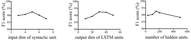
Figure 6: The effects of hyperparameters of the base neural network.

5.3 Relation Prediction

New relations generated via ssCRP only contain a small number of seed instances. To populate relations, part of unlabeled entity pairs will be assigned with labels based on model prediction, and added to the training set. To avoid error propagation, the algorithm requires that only if the prediction of DSNN is highly confident for an entity pair, can we add it to the training set.

Consider the distribution [Pr(r1|e1, e2), . . . ,Pr(rK+l|e1, e2)] for entity pair (e1, e2). If it is “near

uniform”, none of the existing relation labels are confident enough to be the perfect fit. Goodness-of-fit tests are able to determine if the prediction follows uniform distribution (e.g. Kolmogorov-Smirnov test), but experiments show they do not work in this scenario (refer to Section 6.3). In this paper, we define a heuristic “Max-SecondMax” value to estimate the confidence score of a prediction:

conf(e1, e2) =

max([Pr(r1|e1, e2), . . . ,Pr(rK+l|e1, e2)])

secondMax([Pr(r1|e1, e2), . . . ,Pr(rK+l|e1, e2)])

(5)

where secondMax(·)is the second largest value of probabilities. Ifconf(e1, e2)is no less than a given

thresholdτ, the label with the highest probability is indeed a convincing prediction. Such entity pairs will be added to labeled data together with their labels.

6 Experiments

In this section, we conduct extensive experiments for ERC task to evaluate our method and compare it with state-of-the-art approaches.

6.1 Datasets

We use distant supervision (Mintz et al., 2009) to create datasets. We choose four relations from an entertainment knowledge graph (Fan et al., 2017), and extract texts from Chinese Wikipedia where two entities from the same pair have joint occurrence. We manually check the correctness of relation labeling and remove annotation errors. In total, we have 3480 sentences with annotated entity pairs and relations, and spilt them into training data, testing data and validation data, with the proportion of 70%, 20% and 10%. The statistics of labeled data are summarized in Table 1. Similarly, two entities which do not appear in pairs of pre-defined relations are used for harvesting unlabeled data, which contains 3161 sentences.

6.2 Evaluation of Relation Classification

We implement base neural network with Keras3and use dependency parsing results generated by pyltp4. The word embeddings are initialized as 50 dimensions, trained on Chinese Wikipedia dump5 _{via the}

Skip-gram model (Mikolov et al., 2013).

3

https://github.com/fchollet/keras/tree/master/keras 4

http://www.ltp-cloud.com/

Classifier Feature set F1 (%)

logistic regression/ SVM

entity pairs (add) 77.3/ 77.4 entity pairs (sub) 75.9/ 80.8 entity pairs (concat) 89.0/ 87.5 syntactic units, entity pairs (concat) 84.9/ 82.5 context words, entity pairs (concat) 87.6/ 86.6 syntactic units, context words 89.2/ 87.8 syntactic units, context words, entity pairs (concat) 89.9/ 88.0 Shwartz et al. (Shwartz et al., 2016) shortest dependency path, entity pairs 65.3 Zeng et al. (Zeng et al., 2014) context words, entity pairs 81.5 RNN+E syntactic units, entity pairs (concat) 66.8 CNN+E context words, entity pairs (concat) 91.4 Full implementation syntactic units, context words, entity pairs (concat) 92.2

Table 2: Classifiers with their feature sets and F1 score in relation classification.

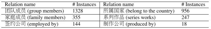
Relation name # Instances Relation name # Instances 团队成_员(group members) 1328 所属国家(belong to the country) 956 家庭成_员(family members) 355 系列作品(series works) 247 签_约公_司(employed by) 144 制作公_司(produced by) 18

Table 3: Semantic relations discovered via ssCRP.

We first study the effects of hyperparameters, i.e., the input dimension of syntactic unit dsyn, the

output dimension of LSTM unitsdlstmand the number of convolutional hidden unitsh. We tune these

hyperparameters on the validation set and illustrate the F1 scores with different settings in Fig. 6. As we can see, the best performance is achieved whendsyn = 5anddlstm= 30. The base neural network

shows signs of overfitting withhlarger than 150. We heuristically set the window sizek= 5and train the network with 0.5 weightedL2regularization.

The second part is to evaluate the effectiveness of the proposed features. We implement several state-of-the-art methods of representing the embeddings of entity pairs: concatenation~ve1 ⊕~ve2, difference

~ve1−~ve2 and sum~ve1+~ve2 model (Baroni et al., 2012; Roller et al., 2014; Mirza and Tonelli, 2016). We train logistic regression and SVM with the combination of the above features. As Table 2 shows, both classifiers achieve the highest F1 scores when trained with all three features. Similar to observations (Mirza and Tonelli, 2016), the concatenated embeddings of entity pairs are the most effective.

The third part is the comparison of our model and other approaches. We implement the CNN-based model (Zeng et al., 2014) and keep the way they use features. Another competitor is the RNN-based model for hypernymy detection (Shwartz et al., 2016), which is modified slightly to classify more gen-eralized semantic relations. We also evaluate the variations of base neural network during iterations, e.g. removing LSTM units (CNN+E) or the convolution layer (RNN+E). The results shown in Table 2 prove that our model has the best performance. The CNN-based models such as CNN+E and model (Zeng et al., 2014) are both significantly effective than RNN-based models, e.g. RNN+E and model (Shwartz et al., 2016). It suggests that lexical features are more effective than syntactic features. The embedding layer improves the performance in either situation due to the use of semantic features.

6.3 Evaluation of Relation Discovery

We first introduce the semantic relations found during the relation discovery process. Table 3 summarizes six relations discovered via ssCRP, containing 3048 instances. The sizes of relations are unbalanced due to the random selection of entity pairs in order to construct unlabeled data automatically.

0.0 0.2 0.4 0.6 0.8 1.0 0

50 100

k

top-k

precision

0.0 0.2 0.4 0.6 0.8 1.0 0

50 100

k

top-k

precision

0.0 0.2 0.4 0.6 0.8 1.0 0

50

100 ssCRP_{Seeded KMeans} EM-based Naive Bayes ssCRP w/o prediction

Logistic ssCRP Exp ssCRP ssCRP w/o tables

k

top-k

precision

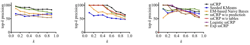
Figure 7: The top-kprecisions (%) of three relations (series works, produced by, employed by) generated by various methods with differentk.

Algorithm # Instances Precision (%) Recall (%) F1 (%) Fit ssCRP 3161 31.0 35.7 33.2 Exploratory EM-based Naive Bayes 3161 70.7 40.2 52.8 Exploratory seeded KMeans 3161 80.5 53.0 63.9 ssCRP w/o tables 593 66.6 60.4 63.3 ssCRP w/o prediction 903 83.7 61.0 70.6 Exp ssCRP 3161 77.9 66.7 71.9 Logistic ssCRP 3161 81.4 66.9 73.0 Full implementation of ssCRP 3048 83.1 68.4 75.0

Table 4: Performance of different algorithms for relation discovery.

classes. The E-step starts with a random initialization of class assignment, and M-step retrains the model until convergence. We also try several variations of our model. For example, we replace the magnifying function with logistic decay (Logistic ssCRP) or exponential decay (Exp ssCRP) proposed in (Blei and Frazier, 2010). In relation prediction process, we make a comparison between the “Max-SecondMax” criterion and goodness-of-fit models such as Kolmogorov-Smirnov test with significance level of 0.05 (Fit ssCRP). Populating new clusters is essential for our model, so we conduct experiments of two related strategies, e.g. not allowing to join existing tables (ssCRP w/o tables) or removing the relation prediction process (ssCRP w/o prediction). We setτ = 2for all variations, fine tuned over the validation set.

The first experiment presents the top-k precision of newly found relations. Relation instances are sorted according to the cosine similarity between its embedding and averaged relation embedding. We ask human annotator to label whether the extracted top-k relations are correct or not, and evaluate the top-kprecision withkranging from 0.1 to 0.9, and show the results in Fig. 7. The illustrated relations achieve the best performance when they are generated by ssCRP, compared with other baseline models6. We heuristically choosek= 0.4because the precision drops relatively faster whenkis larger.

Next, we design a pairwise experiment to evaluate this non-standard clustering task. We manually construct a standard testing dataset by sampling pairs of instances from unlabeled data. For two entity pairsxi andxj with their respective sentences, we use the domain knowledge graph (Fan et al., 2017)

as the ground truth to determine whether xi andxj have the same relation. We use Precision, Recall

and F1 score as the evaluation metrics. We present the performance of ssCRP and other baseline models in Table 4. For two baseline models, exploratory seeded KMeans performs better than exploratory EM-based Naive Bayes. Experiments of ssCRP variations prove the effectiveness of our specially designed magnifying function and “Max-SecondMax” criterion. The reason that goodness-of-fit models fail is that they are sensitive to check whether the data follows uniform distribution or not, while our purpose is to select those with prominent peaks. Thus non-confident relation labels are assigned to unlabeled entity pairs roughly, increasing the number of false positive instances. For the strategies of table assignment and relation prediction process, the experimental results show that they not only populate new relations, but also improve the overall performance.

6.3.1 Error Analysis

To further obtain additional insights into our method, we study the errors in newly found relations and present three types of errors. A frequent type of confusion happens when entity pairs are closely related

under the same topic but not by the same relation, which accounts for 63.4% errors. For example, two entities involved with cooperation relation are be misclassified to the relation “团队成员 (group members)”. Another 23.7% bad cases are due to the false positive results of NER where common nouns are mistaken as named entities, especially for specific names such as “黎明(Ming Li, which also has the meaning of dawn)”. The rest of errors result from the mixture of different grains of relation types. We observe that the relation “所属国家(belong to the country)” contains a few instances wheree2is not a

country but a finer-grained city or a district.

7 Conclusion

In this paper, we propose the task of ERC to address the problem of domain-specific knowledge ac-quisition. We propose a DSNN model to address the task, consisting of three modules, an integrated base neural network for relation classification, a similarity-based clustering algorithm ssCRP to generate new relations and constrained relation prediction process with the purpose of populating new relations. Extensive experiments are conducted to evaluate the effectiveness of our approach.

Acknowledgements

This work is partially supported by the National Key Research and Development Program of China under Grant No. 2016YFB1000904.

References

David J Aldous. 1985. Exchangeability and related topics. Springer Berlin Heidelberg.

Michele Banko, Michael J. Cafarella, Stephen Soderland, Matthew Broadhead, and Oren Etzioni. 2007. Open information extraction from the web. InIJCAI, pages 2670–2676.

Marco Baroni, Raffaella Bernardi, Ngoc-Quynh Do, and Chung-chieh Shan. 2012. Entailment above the word level in distributional semantics. InEACL, pages 23–32.

Sugato Basu, Arindam Banerjee, and Raymond J. Mooney. 2002. Semi-supervised clustering by seeding. In ICML, pages 27–34.

David M. Blei and Peter I. Frazier. 2010. Distance dependent chinese restaurant processes. InICML, pages 87–94.

Razvan C. Bunescu and Raymond J. Mooney. 2005. A shortest path dependency kernel for relation extraction. In HLT/EMNLP, pages 724–731.

Rui Cai, Xiaodong Zhang, and Houfeng Wang. 2016. Bidirectional recurrent convolutional neural network for relation classification. InACL, pages 756–765.

Bhavana Bharat Dalvi, William W. Cohen, and Jamie Callan. 2013. Exploratory learning. InECML/PKDD, pages 128–143.

Oren Etzioni, Anthony Fader, Janara Christensen, Stephen Soderland, and Mausam. 2011. Open information extraction: The second generation. InIJCAI, pages 3–10.

Yan Fan, Chengyu Wang, Guomin Zhou, and Xiaofeng He. 2017. Dkgbuilder: An architecture for building a domain knowledge graph from scratch. InDASFAA, pages 663–667.

Marti A. Hearst. 1992. Automatic acquisition of hyponyms from large text corpora. InCOLING, pages 539–545.

Sepp Hochreiter and J¨urgen Schmidhuber. 1997. Long short-term memory. Neural Computation, 9(8):1735– 1780.

Nanda Kambhatla. 2004. Combining lexical, syntactic, and semantic features with maximum entropy models for extracting relations. InACL, page 22.

Mike Mintz, Steven Bills, Rion Snow, and Daniel Jurafsky. 2009. Distant supervision for relation extraction without labeled data. InACL, pages 1003–1011.

Paramita Mirza and Sara Tonelli. 2016. On the contribution of word embeddings to temporal relation classifica-tion. InCOLING, pages 2818–2828.

Kamal Nigam, Andrew McCallum, Sebastian Thrun, and Tom M. Mitchell. 2000. Text classification from labeled and unlabeled documents using EM. Machine Learning, 39(2/3):103–134.

Jeffrey Pennington, Richard Socher, and Christopher D. Manning. 2014. Glove: Global vectors for word repre-sentation. InEMNLP, pages 1532–1543.

Likun Qiu and Yue Zhang. 2014. ZORE: A syntax-based system for chinese open relation extraction. InEMNLP, pages 1870–1880.

Desh Raj, Sunil Kumar Sahu, and Ashish Anand. 2017. Learning local and global contexts using a convolutional recurrent network model for relation classification in biomedical text. InCoNLL 2017, pages 311–321.

Carl Edward Rasmussen. 1999. The infinite gaussian mixture model. InNIPS, pages 554–560.

Sebastian Riedel, Limin Yao, Andrew McCallum, and Benjamin M. Marlin. 2013. Relation extraction with matrix factorization and universal schemas. InHLT-NAACL, pages 74–84.

Stephen Roller, Katrin Erk, and Gemma Boleda. 2014. Inclusive yet selective: Supervised distributional hyper-nymy detection. InCOLING, pages 1025–1036.

Vered Shwartz, Yoav Goldberg, and Ido Dagan. 2016. Improving hypernymy detection with an integrated path-based and distributional method. InACL, pages 2389–2398.

Ngoc Thang Vu, Heike Adel, Pankaj Gupta, and Hinrich Sch¨utze. 2016. Combining recurrent and convolutional neural networks for relation classification. InHLT-NAACL, pages 534–539.

Chengyu Wang and Xiaofeng He. 2016. Chinese hypernym-hyponym extraction from user generated categories. InCOLING, pages 1350–1361.

Chengyu Wang, Junchi Yan, Aoying Zhou, and Xiaofeng He. 2017. Transductive non-linear learning for chinese hypernym prediction. InACL, pages 1394–1404.

Fei Wu and Daniel S. Weld. 2007. Autonomously semantifying wikipedia. InCIKM, pages 41–50.

Yan Xu, Lili Mou, Ge Li, Yunchuan Chen, Hao Peng, and Zhi Jin. 2015. Classifying relations via long short term memory networks along shortest dependency paths. InEMNLP, pages 1785–1794.

Daojian Zeng, Kang Liu, Siwei Lai, Guangyou Zhou, and Jun Zhao. 2014. Relation classification via convolu-tional deep neural network. InCOLING, pages 2335–2344.