Development of a Partially Bracketed Corpus with
Part-of-Speech Information Only
Hsin-Hsi Chen
and
Yue-Shi Lee
Department of Computer Science and Information Engineering
National Taiwan University
Taipei, Taiwan, R.O.C.
E-mail: [email protected]
Abstract
Resea/ch based on a treebank is active for many natural language applications. However, the work to build a large scale treebank is laborious and tedious. This paper proposes a probabilistic chunker to help the development of a partially bracketed corpus. The chunker partitions the part-of-speech sequence into segments called chunks. Rather than using a treebank as our training corpus, a corpus which is tagged with part-of-speech information only is used. The experimental results show the probabilistic chunker has more than 92% correct rate in outside test. The well-formed partially bracketed corpus is a milestone in the development of a treebank. Besides, the simple but effective chunker can also be applied to many natural language applications.
1. Introduction
Research based on a treebank, i.e., a corpus annotated with syntactic structures, is active for many natural language applications [1-5]. Framis [1] proposes a methodology to extract selectional restrictions at a variable level of abstraction from the Penn Treebank. Chen and Chen [2] propose a probabilistic chunker to decide the implicit boundaries of constituents and utilize the linguistic knowledge to extract the noun phrases by a finite state mechanism. In their study, Susanne Corpus is used as a trainmg corpus for their chunker. Pocock and Atwell [3] investigate statistical grammars extracted from Spoken English Corpus (SEC), and apply these grammars to find the grammatically optimal path through a word lattice. The stochastic parsers are also developed in [4,5]. All these applications employ the syntactic information extracted from different treebanks and show the satisfactory results.
However, the work to build a large scale treebank is laborious and tedious. Very few large-scale treebanks are currently available especially for languages other than English. In this paper, we propose a probabilistic chunker to help the development of a partially bracketed corpus, i.e., a simpler version of a treebank. The chunker partitions the part-of-speech sequence into segments called chunks. Rather than using a treebank as our training corpus, a corpus which is tagged with part-of-speech information only is used. In the following sections we first introduce the experimental framework of our model. Lancaster- Oslo/Bergen (LOB) Corpus and Susanne Corpus are adopted. Then a tag mapper and a probabilistic chunker are described. Before concluding the experimental results are demonstrated.
2. Experimental Framework
speech sequence P is generated. The output of the tagger is the input of the chunker. The probabilistic chunker partitions P into C, i.e., a sequence of chunks. Each chunk contains one or more parts of speech.
[image:2.612.119.494.276.399.2] [image:2.612.93.512.606.723.2]Consider the example "Attorneys for the mayor said that an amicable property settlement has been agreed upon .". This 15-word sentence is input to the part-of-speech tagger and a part-of-speech sequence "NNS IN ATI NPT VBD CS AT JJ NN NN HVZ BEN VBN IN ." is generated. The probabilistic chunker then partitions this sequence into several chunks. The chunked result is shown as follows.
[ N N S ] [ I N A T I N P T ] [ V B D ] [ C S ] [ A T ] [ J J N N N N ] [ HVZ BEN ] [ V B N ] [ I N ] [ . ]
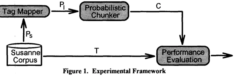
However, the pei-formance evaluation of the chunker is a sticky work. To evaluate the performance of the chunker, Susanne Corpus, which is a modified and condensed version of Brown Corpus, is adopted. But, the tagging sets [6,7] of LOB Corpus and Susanne Corpus are different. The latter has finer tags than the former. Thus, a tag mapper is introduced in the experimental framework shown as Figure 1.
~!.:: . r . ~ : . . ~ . . : ~ :~.j -~':
~'~-~ ~ "~-:'~:"~ "::::'::::~:'~:':~:i':::: .::i'::::'~': -:" ... ::::':':~:::::':::::'::::::~::::~: ~ ... i :~:::: :::::::::::"~!~:!:'~:" ~'| a i ~ . ~ .:.i~ ~ :':: :'~ "":" ":':"~ ~:':':':':':':':':":" ::'~:'~ ~ ~ ":: ... :::::" ":':':~ :~'~" li ~.~.ii::.:i "" ":':":':':':':':'~ ~ ~.~ ~:i~il ~...:~.~ |
C
Figure 1. Experimental Framework
In our experiments, the test sentence Ps comes from Susanne Corpus. It is a part-of-speech sequence. The corresponding syntactic structure T is regarded as an evaluation criterion for the probabilistic chunker. It is sent to the performance evaluation model. The tag mapper in this figure is used to transform the Susanne part-of-speech into LOB part-of-speech. Through the tag mapper, Ps is converted into PI. Then, PI is input to the probabilistic chunker and a chunk sequence C is produced. Finally, the performance evaluation model reports the evaluation results according to C and T.
3. A Tag Mapper
The tagging set of Susanne Corpus is extended and modified from LOB Corpus. They have 424 and 153 tags, respectively. To map a Susanne tag into a LOB tag manually is a tedious work. Thus, an automatic tag mapping algorithm is provided. By our investigation, we found that words are good clues to relate these two tagging sets. Therefore, the first step in automatic tag mapping is to collect words from Susanne Corpus for each Susanne tag. Table 1 lists some examples.
Table 1. Words Extracted from Susanne Corpus for Some Susanne Tags
SusannelTags Words LOB Tags
CC and plus & And ond CC
IW with WITHOUT without WITH With IN NNlux
NN 2
WM
physics math politics mathematics Athletics associates
<apos>m am ai <bbold> <bital> r r L
Column three in Table 1 denotes the correct mapping to LOB tags. The second step is to find the corresponding LOB tags from LOB Corpus for each word collected at the first step. Table 2 shows the sample results.
Table 2. LOB Tags Extracted from LOB Corpus for Each Word in Table 1
Susanne Tags CC IW NNlux
NNJ2 VBM YTL
Words (LOB Tags)
and ( CC RB" RB NC ) plus ( IN JJ NN &FW ) & ( CC ) with ( IN IN" RI NC ) without ( IN RI )
physics ( NN ) politics ( NN NNS ) mathematics ( NN ) associates ( NNS VBZ )
am ( BEM &FW ) ai ( HVZ BEZ BER )
Those words which cannot be found in LOB Corpus are removed. Symbol * denotes that all the words cannot be found in LOB Corpus. The third step is to find the corresponding LOB tag for each Susanne tag. For each Susanne tag, the frequency of LOB tags is calculated and the most frequent LOB tag is regarded as the result. For example, LOB tags NN and NNS in row three of Table 2 appear three and one times, respectively. Thus, Susanne tag NNlux is mapped to LOB tag NN. After examining all the Susanne tags by these three steps, three cases have to be considered:
(1) Unique Tag. Only one LOB tag remains.
(2) Multiple Tags. More than one LOB tags remain. (3) No Match.
When all the words extracted from Susanne Corpus for a Susanne tag cannot be found in LOB Corpus, the Susanne tag is mapped to "No Match". Some of these words are characteristic words such as YTL 1.
The experimental results are shown in Table 3.
Table 3. Experimental Results for Ta:
Mapping Types Subtypes
Unique Tag Correct
Wrong Multiple Tags Include
Exclude
No Match Correct
Wrong
Mapping
Number of Mapping 151
7 113
3 10 26
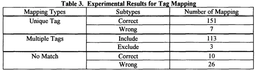
In Table 3, "Include" denotes that the correct tag belongs to the remaining multiple tags and " Exclude" denotes that the correct tag is not mcluded in the remaining tags. Note that the ditto tags are not considered in this experiment. This is because the mapping for ditto tags can be obtained by human easily. Therefore, only 310 Susanne tags are resolved in this experiment. The experimental results show that the number of multiple tags is large. Thus, two heuristic rules are introduced to reduce the number of multiple tags.
[image:3.612.103.525.139.252.2] [image:3.612.100.525.451.567.2]First, those LOB tags which are similar to Susanne tag are selected. For example, Susanne tag NNJ2 can be mapped tO LOB tags NNS or VBZ in the above experiment. NNS has two common characters with NNJ2, so that Susanne tag NNJ2 is mapped to LOB tag NNS. Under this heuristic rule, the experimental results are showia m Table 4.
Table 4. Experimental Results After Applying the First Heuristic Rule
Mapping Types Unique Tag MUltiple Tags No Match Subtypes Correct Wrong Include Exclude Correct Wrong
Number of Mappin 8 222
22 28
10 26
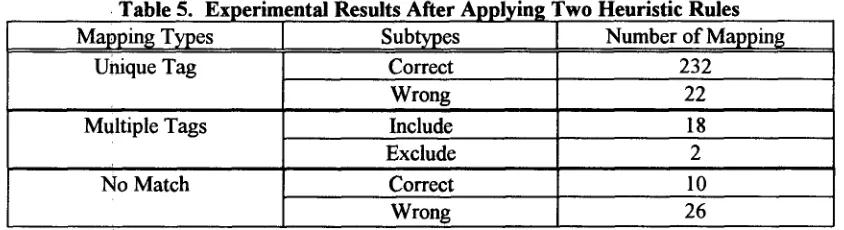
Next, let us consider an example. Susanne tag IW can be mapped to LOB tags IN or RI in the above experiment. Thus, the first heuristic rule has no effects. We examine the tag mapping for the preceding and subsequent three tags of 1W. They are listed as follows.
(-1) Susanne Tag lit is mapped to (-2) Susanne Tag IIx is mapped to (-3) Susanne Tag IO is mapped to (**) Susanne Tag IW is mapped to (+2) Susanne Tag JB is mapped to (+3) Susanne Tag JBo is mapped to
LOB Tag IN. LOB Tag IN. LOB Tag IN. LOB Tag IN RI. LOB Tag JJ. LOB Tag AP.
Note that only tags which have the same first character as IW are considered, that is,. only (-I), (-2) and (-3) are considered. In these three mappings, LOB tag IN is the most frequent and the only one mapping, and IN is a candidate for IW. Thus, Susanne tag IW is mapped to LOB tag IN. The above procedure forms the second heuristic rule. The experimental results after applying two heuristic rules are shown as follows.
Table 5. Experimental Results After Applying Two Heuristic
Mapping Types Unique Tag
Multiple Tags
No Match
Subtypes Numbe r Correct Wrong Include Exclude Correct Wrong Rules of Mapping 232 22 18 10 26
Three tags - say, FA, FB and GG, must be treated in particular. For example, Susanne Corpus tags genitive case noun as [John NP 's_GG], but LOB Corpus tags it as [John's_PN$]. Two Susanne tags may be mapped into One LOB tag. Ignoring these three special tags, only nineteen Susanne tags have wrong mapping in Uniq0e-Tag case.
4. A Probabilistic Chunker
[image:4.612.88.508.163.277.2] [image:4.612.89.511.473.588.2]Table 6. A Contingency Table Word w 1
Word w 2 a b
c d
Cell a counts the number o f sentences that contain both w I and w 2. Cell b (c) counts the number of
sentences that contain w 2 (Wl) but not w I (w2). Cell d counts the number o f sentences that does not
contain both w 1 and w 2. That is, if N is the total number o f sentences, d=N-a-b-c. Based on this
contingency table,
(~2
is defined as follows:( a * d + b ' c ) 2
42 = ( a + b ) * ( a + c ) * ( b + d ) * ( c + d )
(I) 2 is bounded between 0 and 1. For different applications, there are different definitions for the contingency table. Instead of using the above definition, a modified version is shown as follows.
Definition 1: (For Two Parts of Speech)
a=F(Pl,P2)
b=F(P2)-F(P l,p 2 )
c=F(P 1)-F(p l,P2) d=N-a-b-c
where Pi denotes part-of-speech i,
F(p 1,P2) is the frequency o f which P2 follows p 1,
F(Pl) and F(P2) are the frequencies o f Pl and P2, and
N is the corpus size in terms o f the number of words in training corpus.
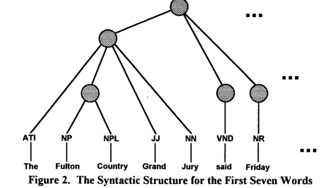
Based on this definition and ~2 measure, consider the sentence "The Fulton County Grand Jury said Friday an investigation ...", which has tag sequence "ATI NP NPL JJ NN VBD NR AT NN ...". Its syntactic structure for the first seven words is shown in Figure 2.
ATI NP
I
I
[image:5.612.215.419.85.148.2]The Fulton
Figure 2.
NPL JJ NN VND NR
I
1
1
1
I
Country Grand Jury said Friday
mum
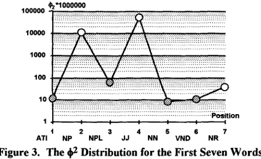
[image:5.612.145.463.489.675.2]The 4 2 distribution for these parts of speech is shown in Figure 3. Position i (x axis) is the location between parts of speech Pi and Pi+ 1'
"1000000
10000
1oo
1 tion
t 2 3 4 5 6 7
ATI NP NPL JJ NN VND NR
Figure 3. The ~2 Distribution for the First Seven Words
Figure 3 shows that there are four local minimal positions, i.e., positions 1, 3, 5 and 6. They can be regarded as the boundaries of chunks. That is, ATI and NP belong to different chunks. Similarly, (NPL and JJ), (NN and VND) and (VND and NR) have the same situation. Let us discuss these concepts formally. For a!probabilistic chunker, the generalized contingency table is defined as follows.
Definition 2: (For Two Chunks) a=F(cl,c 2)
b=F(c2)-F(cl,c 2)
c=F(Cl)-F(cl,c 2) d=N-a-b-c
where c i denotes chunk i,
.F(cl,c2) is the frequency of which c 2 follows el,
F(cl) and F(c2) are the frequencies o f c 1 and c2, and
N is the corpus size m terms of the number of words in training corpus.
Let the tag sequence P be P l, P2, .-., Pn. Assume there are two possible chunked results. The first is
composed o f t w 0 chunks, i.e., [Pl, P2 ... Pi] and [Pi+l, Pi+2, --., Pn], and is regarded as a correct result.
The second is also composed of two chunks, i.e., [Pl, P2, -.., Pi-l] and [Pi, Pi+l, -.., Pn], but is regarded as
a wrong result, iSince [Pl, P2, ..., Pi] is a chunk, [Pl, P2 ... Pi-1] is very likely to be followed by Pi. In other words,
F([Pl, P2, ..-, Pi-1]) ~ F([Pl, P2 .... , Pi]) ... (1)
Similarly,
F([Pi+I, Pi+2, --', Pn]) '~' F([Pi+2, Pi+3, ---, Pn])
Because Pi and Pi+l are in two different chunks,
F([Pi, Pi+l,.--., Pn]) << F([Pi+I, Pi+2, .-., Pn]) ... (2)
Similarly,
[image:6.612.178.433.141.297.2]For the first chunked result, we can obtain the following contingency table:
a# = F([Pl, P2, -.., Pi],[Pi+l, Pi+2, ..-, Pn])
b# = F([pl, P2, ---, Pi]) - F([Pl, P2, .-., Pi],[Pi+l, Pi+2, ..., Pn])
c# = F([Pi+I, Pi+2, .-., Pn]) - F([Pl, P2 ... Pi],[Pi+l, Pi+2, .-., Pn])
d # = N - a # - b # - c #
Similarly, the following contingency table is obtained for the second chunked result:
a& = F([pl, P2 . . . . , Pi-l],[Pi, Pi+l, ..., Pn])
b& = F([Pl, P2, ..., Pi-l]) - F([Pl, P2, ..., P i-l],[Pi, Pi+2, ..., Pn])
c& = F([Pi, Pi+l, --., Pn]) " F ( [ P l , P2 .... , P i-l],[Pi, Pi+2, ..., Pn])
d & = N -a & - b & - c &
It is obvious that a # = a &. By formula (1), we know that b # ~ b &. By formula (2), we can derive c # >> c &. Since N >> a, b and c, d # ,~, d &. Therefore,
(a # * d # _ b # * c #) << (a & * d & _ b & * c &)
(a # + b #) ~ (a & + b &) (a # + c #) >> (a & + c &) (b # + d # ) ,~, (b & + d &)
(c # + d #) ~ (c & + d &)
and
d ( [ P , , P2, ..., P,],[P,+., P,+2, .--, P.])
( a ' * d" - b"* c") 2
(a" + b')* (a" + c")* (b" + d')* (c" + d")
<< ( a ~ * d ~ _ b ~ * c ~ ) 2
(a & + b ~) * (a ~ + c ~) * (b ~ + d ~) * (c ~ + d ~)
= ~2([pl, P2,---, Pi-l],[Pi, PJ+i, ..., P,])
The above derivation tells us: the local minimums o f the ~b 2 distribution denote plausible boundaries o f two chunks. To simplify Definition 2, Definitions 3 and 4 are formulated.
D e f i n i t i o n 3: ( F o r T w o P a r t s of Speech) a = F([Pi],[Pi+l])
b = F([Pi]) - F([Pi],[Pi+l]) e = F([Pi+l]) - F([Pi],[Pi+l]) d = N - a - b - c
where Pi denotes part-of-speech i,
F([Pi],[Pi+l] ) is the frequency o f which Pi+l follows Pi, F([Pi] ) and F([Pi+l]) are the frequencies o f Pi and Pi+l, and
It is clear that Definition 3 is the same as Definition 1. Based on Definitions 3, the probabilistic chunker is presented as follows. Note that N is the length of the tag sequence and the last chunk is always a one-tag chunk (punctuation).
Probabilistic Chunker(A_Sequence Of Tags)
Begin
Output("["); Position=l;
Calculate ~2 a for Current Position By Definition 3; Position=Position+ 1;
While(Position<N)
Begin
Calculate ,l,2b for Current Position By Definition 3; Output(A_Sequence Of Tags[Position-l]);
If (,l,2a < ,I,2b) Then Output("][");
~2a=(I)2b;
Position=Position+ l;
End End
Output(A_Sequence Of Tags[N-l]); Output("][");
Output(A_Sequence Of Tags[N]); Output("]");
Definition 4: (For Three Parts of Speech)
Left Chunk
a = F([pi, Pi+l],[Pi+2])
b = F([Pi+2]) - F([pi, Pi+l],[Pi+2]) c = F([Pi, Pi+l]) "F([Pi, Pi+l],[Pi+2]) d = N - a - b - c
where Pi denotes part-of-speech i,
F([Pi, Pi+l],[Pi+2]) is the frequency of which Pi+l,Pi+2 follows Pi, F([pi, Pi+l]) and F([Pi+2]) are the frequencies of (pi, Pi+l) and Pi+2, and N is the corpus size m terms of the number of words in training corpus.
Right Chunk
a = F([Pi],[pi+ 1, Pi+2])
b = F([Pi+l , Pi+2]) - F([Pi],[Pi+I, Pi+2]) c = F([Pi]) - F([Pi],[Pi+l, Pi+2])
d = N - a - b - c
where Pi denotes part-of-speech i,
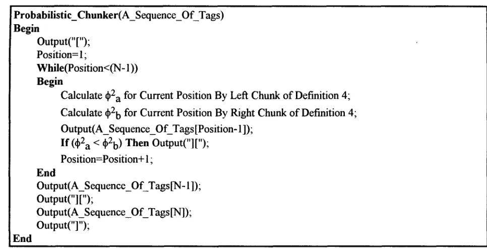
Based on Definitions 4, the probabilistic chunker is presented as follows.
Probabilistic_Chunker(A_Sequence Of Tags)
Begin
Output("["); Position= 1;
While(Position<(N- 1))
Begin
Calculate qb2a for Current Position By Left Chunk of Definition 4; Calculate dp2b for Current Position By Right Chunk of Definition 4; Output(A_Sequence Of Tags[Position-l]);
If (dp2 a < dp2b) Then Output("]["); Position=Position+ 1;
End
Output(A_Sequence Of Tags[N-l]); Output("][");
Output(A_Sequence Of Tags[N]); Output("]");
End
Probabilistic chunker based on Definition 3 concerns the dp 2 distribution between two parts of speech. For each while loop, probabilistic chunker based on Definition 4 processes three parts of speech and concerns the dp 2 distribution between them.
5. Experimental Results
LOB Corpus, which is a million-word collection of present-day British English texts, is adopted as the source of training data. Susanne Corpus is adopted as the source of testing data for evaluating the performance of our probabilistic chunker. This corpus contains one tenth of Brown Corpus, but involves more syntactic and semantic information than Brown Corpus.
For evaluating the performance, a criterion [2], i.e., the content of each chunk should be dominated by one non-terminal node in Susanne parse field, is adopted. The performance evaluation model compares the chunked result C with the corresponding syntactic structure T. Accordmg to this criterion, the experimental results for Definitions 3 and 4 are shown in Table 7 as follows.
[image:9.612.67.550.107.353.2]File
Table 7. Experimental Results for Definition 3 and 4
Correct Rate for Definition 3
II
Correct Rate for Definition 4A0I 80.31% 79.71%
G0I 79.28% 79.72%
J01 76.42% ! 77.17%
N01 87.82% 90.10%
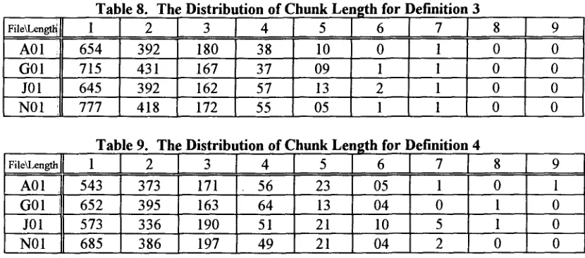
The experimental results demonstrate that Definition 4 (three parts of speech) is more powerful than Definition 3 (two parts of speech). Assume the chunk length is the number of tags in a chunk. The distribution of Chunk length is listed in Tables 8 and 9.
Table 8. The Distribution of Chunk Length for Definition 3
1
I 2
3 1 4 1 5
6
I 7
8 1
9A01 i 654 392 180 38 10 0 1 0 0
G01 715 431 167 37 09 1 I 0 0
J01 i 645 392 162 57 13 2 1 0 0
N01 777 418 172 55 05 1 1 0 0
Table
1
I
A01 543 G01 652 J01 573 N01 685
9 . ' ]
373 395 336 386
The Distribution of Chunk Length for Definition 4
I 3 1 4
5 1 6 1 7
8
171 56 23 05 1 0
163 64 13 04 0 1
190 51 21 10 5 1
197 49 21 04 2 0
One-tag chunks cover about 50%. We further analyze what grammatical components constitute the one- tag chunks and find that most of the one-tag chunks contam punctuation marks, nouns and verbs. This is because proper name forms the bare subject or object. Verb is presented in the form of third person and singular, past tense, or base form. These three cases form about 62% of one-tag chunks.
By analyzing the error chunked results, we find that many errors result from conjunctions. Besides, some tags cannot be located at the end of the chunks. Therefore, the heuristic rule is applied to improve the performance. The tags that cannot be located at the end of chunks are listed as follows:
(01) AT (Singular Article) (03) BED (were)
(05) BEG (being) (07) BER (are, 're)
(09) CC (Coordinating Conjunction) (11) IN (Preposition)
(13) W D T R (WH-Determiner)
(02) ATI (Singular or Plural Article) (04) BEDZ (was)
(06) BEM (am, 'm) (08) BEZ (is, 's)
(10) CS (Subordinating Conjunction) (12) PP$ (Possessive Determiner)
Applying this heuristic rule, the experimental results are listed in Table 10. It shows the usefulness of the heuristic rulel The performance increases about 10%.
Table 10. Ex
File i A01 G01 J01 N01 Average
mrimental Results after Applyin
[ Correct Rate for Definition 3 92.39%
the Heuristic Rule
Correct Rate for Definition 4 89.19%
93.15% 90.92%
91.30% 89.89%
94.86% 92.95%
[image:10.612.100.515.148.331.2] [image:10.612.97.517.603.700.2]6. Concluding Remarks
To process real text is indispensable for a practical natural language system. Probabilistic method provides a robust way to tackle with the unrestricted text. This paper proposes a probabilistic chunker to help the development of a partially bracketed corpus. Rather than using a treebank as our training corpus, LOB Corpus which is tagged with part-of-speech information only is used. The experimental results show the probabilistic chunker has more than 92% correct rate in outside test. The well-formed partially bracketed corpus is a milestone in the development of a treebank. In addition, the simple but effective chunker can also be applied to many natural language applications such as extracting the predicate-argument structures [9,10], grouping words [11] and gathering collocation [12].
The evaluation criterion adopted in this paper is not very strict. Under a strict criterion, the method proposed in this paper may not be suitable for short-fat trees. That is, it is suitable for tall-thin trees. To solve this problem, a more general definition which considers more parts of speech in contingency table is needed. However, that introduces another problem: the more the general definitions we use, the larger the tagged corpus we need. This paper also presents a tag mapper. It sets up the mapping between different tagging sets. Such an algorithm facilitates the development of a large-scale tagged corpus from different sources. By the way, much more reliable statistic information can be trained from the large-scale tagged corpus, so that the feasibility of the chunker is assured. Besides the above problem, the critical points for local minimum are not obvious in some cases. Thus their determination is also demanded in the future.
References
[1] Framis, F.R. (1994) "An Experiment on Learning Appropriate Selectional Restrictions from a Parsed Corpus,"
Proceedings of COLING,
pp. 769-774, 1994.[2] Chen, K H . and Chen, H.H. (1994) "Extracting Noun Phrases from Large-Scale Texts: A Hybrid Approach and its Automatic Evaluation,"
Proceedings of ACL,
pp. 234-241, 1994.[3] Pocock, R.J. and Atwell, E.S. (1993) "Treebank-Tramed Probabilistic Parsmg of Lattices,"
Technical Report 93. 30,
School of Computer Studies, Leeds University, 1993.[4] Pereira, F. and Schabes, Y. (1992) "Inside-Outside Reestimation from Partially Bracketed Corpora,"
Proceedings of ACL,
pp. 128-135, 1992.[5] Weischedel, R.,
et al.
(1991) "Partial Parsing: A Report of Work in Progress,"Proceedings of
DARPA Speech and Natural Language Workshop,
pp. 204-209, 1991.[6] Sampson, G. (1993) "The Susanne Corpus,"
1CAMEdournal,
17, 125-127, 1993.[7] Johansson, S. (1986)
The Tagged LOB Corpus: Users' Manual,
Bergen: Norwegian Computing Center for Humanities, 1986.[8] Gale, W.A. and Church, K.W. (1991) "Identifying Word Correspondences in Parallel Texts,"
Proceedings of DARPA Speech and Natural Language Workshop,
pp. 152-157, 1991.[9] Church, K.W. (1988) "A Stochastic Parts Program and Noun Phrase Parser for Unrestricted Text,"
Proceedings of Applied Natural Language Processing,
pp. 136-143, 1988.[10] Church, K.W.,
et al.
(1989) "Parsing, Word Association and Typical Predicate-Argument Relations,"Proceedings of Parsing Technologies Workshop,
pp. 389-398, 1989.[11] Hindle, D. (1990) "Noun Classification from Predicate-Argument Structures,"
Proceedings of ACL,
pp. 268-275, 1990.