Heuristic Based Heterogeneous Longest Approximate
Time to End
Algorithm of Scientific Workflows in
Computational Clouds
S.Selvalakshmi
1, S.Vinodkumar
21
Research Scholar ,2Assistant Professor Department of Computer Science Sree Saraswathi Thyagaraja College, Pollachi, Coimbatore, TamilNadu, India -642 107. Email: 1[email protected] , 2[email protected]
Abstract-The elasticity of Cloud infrastructures makes them a suitable platform for execution of deadline-constrained workflow applications, because resources available to the application can be dynamically increased to enable application speedup. Existing research in execution of scientific workflows in Clouds either try to minimize the workflow execution time ignoring deadlines and budgets or focus on the minimization of cost while trying to meet the application deadline. The proposed new scheduling algorithm called Longest Approximate Time to End (LATE) that is highly robust to heterogeneity environment. An especially compelling setting where this occurs is a virtualized data center. We show that cloud scheduler can cause severe performance degradation in heterogeneous environments. We design a new scheduling algorithm, Longest Approximate Time to End (LATE) that is highly robust to heterogeneity.
Index Terms: Scientific workflows, LATE algorithm, Virtualization technology, Virtual Machine
1. INTRODUCTION
Cloud computing is an approach of using computing as utility. Relatively new term for representing collection of resources which are shared, scaled dynamically. Based on “pay as you use” model, resources can be used or released whenever needed. This refers to both, applications as service to users and servers in datacenters which support those services. Cloud computing is a paradigm of distributed computing to provide the customers on-demand, utility based computing services. Cloud itself consists of physical machines in the data centers of cloud providers. Virtualization technology is used on these physical machines to run multiple operating systems simultaneously.
We can define cloud computing as collection of resources (servers in datacenter), which are interconnected with each other and using virtualization technology can be scaled and adapted dynamically. Cloud computing provides customers, to start their business without purchasing any physical hardware, whereas service providers can rent their resources to customers and make their profit. Customers have the opportunity to scale up or down, the resources dynamically to provide QOS for
demand varying application. Cloud computing
enables dynamic and flexible application
provisioning used to virtualization technology. Beneficiaries of cloud computing can be divided into a) cloud computing providers, b) cloud computing customers and c) end-users . Cloud service providers own the physical resources as datacenters. Cloud computing customers; use these resources to provide service to customers and end-users use those services.
1.1 Virtualization Technology
Virtualization technology enables to run multiple
operating systems (or virtual machines)
simultaneously on a single physical machine sharing the same underlying resources. Some of the reason for using virtualization is a) sufficient capability of recent computers to run multiple operating systems, b) using multiple isolated operating systems, resource utilization can be maximized, c) ability to run different operating systems on single physical machine (for example Linux and Windows).
1.2 Cloud scheduling
The primary benefit of moving to Clouds is
scheduling in cloud computing tended to use the direct tasks of users as the overhead application base.
The problem is that there may be no relationship between the overhead application base and the way that different tasks cause overhead costs of resources in cloud systems. For large number of simple tasks this increases the cost and the cost is decreased if we have small number of complex tasks.
1.3 Workflow scheduling
Workflow scheduling is the problem of mapping each task to appropriate resource and allowing the tasks to satisfy some performance criterion. A workflow consists of a sequence of concatenated (connected) steps. Workflow mainly focused with the automation of procedures and also in order to achieve an overall goal thereby files and data are passed between participants according to a defined set of rules. A workflow enables the structuring of applications in a directed acyclic graph (DAG) form where each node represents the task and edges represent the dependencies between the nodes of the applications .A single workflow consists of a set of tasks and each task communicate with another task in the workflow. Workflows are supported by
Workflow Management Systems. Workflow
scheduling discovers resources and allocates tasks on suitable resources. Workflow scheduling plays a vital role in the workflow management. Proper scheduling of workflow can have an efficient impact on the performance of the system. For proper scheduling in workflows various scheduling algorithms is used.
2. RELATED WORK
In [13], Rodrigo N. Calheiros(2014) in this paper, we present the elasticity of Cloud infrastructures makes them a suitable platform for execution of deadline-constrained workflow applications, because resources available to the application can be dynamically increased to enable application speedup.
Existing research in execution of scientific
workflows in Clouds either try to minimize the workflow execution time ignoring deadlines and budgets or focus on the minimization of cost while trying to meet the application deadline. However, they implement limited contingency strategies to correct delays caused by underestimation of tasks execution time or fluctuations in the delivered performance of leased public Cloud resources. To mitigate effects of performance variation of resources on soft deadlines of workflow applications, we
propose an algorithm that uses idle time of provisioned resources and budget surplus to replicate tasks. Simulation experiments with four well-known scientific workflows show that the proposed algorithm increases the likelihood of deadlines being met and reduces the total execution time of applications as the budget available for replication increases.
In [14], A.Hirales-Carbajal, A. Tchernykh, R. Yahyapour (2012) in this paper, we present an experimental study of deterministic non-preemptive multiple workflow scheduling strategies on a Grid. We distinguish twenty five strategies depending on the type and amount of information they require. We analyze scheduling strategies that consist of two and
four stages: labeling, adaptive allocation,
prioritization, and parallel machine scheduling. We apply these strategies in the context of executing the Cybershake, Epigenomics, Genome, Inspiral, LIGO, Montage, and SIPHT workflows applications. In order to provide performance comparison, we performed a joint analysis considering three metrics. A case study is given and corresponding results indicate that well known DAG scheduling algorithms designed for single DAG and single machine settings are not well suited for Grid scheduling scenarios, where user run time estimates are available. We show that the proposed new strategies outperform other strategies in terms of approximation factor, mean critical path waiting time, and critical path slowdown. The robustness of these strategies is also discussed.
End (LATE) that is highly robust to heterogeneity. LATE can improved Hadoop response times by a factor of 2 in clusters of 200 virtual machines on EC2.
3. METHODOLOGY
3.1 LATE Scheduler
Proposed a modified version of speculative execution called Longest Approximate Time to End (LATE) algorithm that uses a different metric to schedule tasks for speculative execution.
Instead of considering the progress made by a task so far, they compute the estimated time remaining, which gives a more clear assessment of a straggling tasks’ impact on the overall job response time. They demonstrated significant improvements by Longest Approximate Time to End (LATE) algorithm over the default speculative execution.
We have designed a new speculative task scheduler by starting from first principles and adding features needed to behave well in a real environment. The primary insight behind our algorithm is as follows: We always speculatively execute the task that we think will finish farthest into the future, because this task provides the greatest opportunity for a speculative copy to overtake the original and reduce the job’s response time. We explain how we estimate a task’s finish time based on progress score below. We call our strategy LATE, for Longest Approximate Time to End. Intuitively, this greedy policy would be optimal if nodes ran at consistent speeds and if there was no cost to launching a speculative task on an otherwise idle node.
Different methods for estimating time left can be plugged into LATE. We currently use a simple heuristic that we found to work well in practice: We estimate the progress rate of each task as Progress Score / T , where T is the amount of time the task has been running for, and then estimate the time to completion as (1 − ProgressScore) /
ProgressRate. This assumes that tasks make progress
at a roughly constant rate. There are cases where this heuristic can fail, which we describe later, but it is effective in typical cloud jobs. To really get the best chance of beating the original task with the speculative task, we should also only launch speculative tasks on fast nodes – not stragglers. We do this through a simple heuristic don’t launch speculative tasks on nodes that are below some
threshold, Slow Node Threshold, of total work performed (sum of progress scores for all succeeded and in progress tasks on the node). This heuristic leads to better performance than assigning a speculative task to the first available node. Another option would be to allow more than one speculative copy of each task, but this wastes resources needlessly.
Finally, to handle the fact that speculative tasks cost resources, we augment the algorithm with two heuristics:
• A cap on the number of speculative tasks
that can be running at once, which we denote SpeculativeCap.
• A SlowTaskThreshold that a task’s progress
rate is compared with to determine whether it is “slow enough” to be speculated upon. This prevents needless speculation when only fast tasks are running.
In summary, the LATE algorithm works as follows: If a node asks for a new task and there are fewer than SpeculativeCap speculative tasks running:
• Ignore the request if the node’s total
progress is below SlowNodeThreshold.
• Rank currently running tasks that are not
currently being speculated by estimated time left.
• Launch a copy of the highest-ranked task
with progress rate below
SlowTaskThreshold.
Like cloud scheduler, we also wait until a task has run for 1 minute before evaluating it for speculation. In practice, we have found that a good choice for the three parameters to LATE is to set the Speculative Cap to 10% of available task slots and set the Slow Node Threshold and Slow Task Threshold to the 25th percentile of node progress and task progress rates respectively. We use these values in our evaluation. We have performed a sensitivity analysis to show that a wide range of thresholds perform well. Finally, we note that unlike cloud scheduler, LATE does not take into account data locality for launching speculative map tasks, although this is a potential extension.
fast node that does not have a local copy of the data. Locality statistics available in cloud validate this assumption.
3.2 Speculative Execution
When a node has an empty task slot, chooses a task for it from one of three categories. First, any failed tasks are given highest priority. This is done to detect when a task fails repeatedly due to a bug and stop the job. Second, non-running tasks are considered. For maps, tasks with data local to the node are chosen first. Finally task to execute speculatively.
To select speculative tasks, monitors task progress using a progress score between 0 and 1. For a map, the progress score is the fraction of input data read. For a reduce task, the execution is divided into three phases, each of which accounts for 1/3 of the score:
• The copy phase, when the task fetches map
outputs.
• The sort phase, when map outputs are sorted
by key.
• The reduce phase, when a user-defined
function is applied to the list of map outputs with each key.
In each phase, the score is the fraction of data processed. The average progress score of each category of tasks (maps and reduces) to define a threshold for speculative execution: When a task’s progress score is less than the average for its category minus 0.2, and the task has run for at least one minute, it is marked as a straggler. All tasks beyond the threshold are considered “equally slow,” and ties between them are broken by data locality.
The scheduler also ensures that at most one speculative copy of each task is running at a time. Finally, when running multiple jobs, uses a FIFO discipline where the earliest submitted job is asked for a task to run, then the second, etc. There is also a priority system for putting jobs into higher-priority queues.
3.3 LATE algorithm
The LATE algorithm uses different
strategies in each phase. The first phase namely, task prioritizing phase is to assign the priority to each task. In this phase, upward rank (given in LATE algorithm) and downward rank values for all tasks are computed. The downward rank is computed by
adding average execution time and communication time starting from entry task to the task excluding execution time of the task for which downward rank is computed. The sum of downward and upward rank is used to assign the priority to each task. Initially, the entry task is the selected task and marked as a critical path task. An immediate successor (of the selected task) that has the highest priority value is selected and it is marked as a critical path task. This process is repeated until the exit node is reached.
In the second phase, task with highest priority is selected for execution. If the selected task in on the critical path, then it is scheduled on the critical path processor. The critical processor is the one that minimizes the cumulative computation costs of the tasks on the critical path; otherwise, it is assigned to a processor, which minimizes the earliest execution finish time of the task.
Improved Longest Approximate Time to End (LATE) is a well-established list scheduling algorithm, which gives higher priority to the workflow task having higher rank value. This rank value is calculated by utilizing average execution time for each task and average communication time between resources of two successive tasks, where the
tasks in the CP(cumulative process) have
comparatively higher rank values. Then, it sorts the tasks by the decreasing order of their rank values, and the task with a higher rank value is given higher priority. In the resource selection phase, tasks are scheduled in the order of their priorities, and each task is assigned to the resource that can complete the task at the earliest time.
Let us consider |Tx| to be the size of task Tx
and R be the set of resources available with average
processing power
|
|
=∑
||
=1 Thus, the average
execution time of the task is defined as
=|||| 1
Let
be the size of data to be transferred betweentask Tx and Ty, and R be the set of resources available
with average data processing capacity
=∑
=1 .
Thus, the average data transfer time for the
task is defined as
=
E(Tx) and D(Txy) are used to calculate the rank of a
task. For an exit task, the rank value is,
rank T = E T 3
Now, the rank value of other tasks in the workflow can be computed recursively on the basis of Equations (1), (2), and (3) and is represented as
Rank T
= E T + max'(∈*+,, -. DT 0 rankT0 4
Because a workflow is represented as a DAG, the rank values of the tasks are calculated by traversing the task graph in a breadth-first search (BFS) manner in the reverse direction of task dependencies (i.e., starting from the exit tasks). The advantage of using LATE over min–min or max–min is that while assigning priorities to the tasks, it considers the entire workflow rather than focusing on only unmapped independent tasks at each step.
3.4 Advantages of LATE
The LATE algorithm has several
advantages. First, it is robust to node heterogeneity, because it will prelaunch only the slowest tasks, and only a small number of tasks. LATE prioritizes among the slow tasks based on how much they hurt job response time. The LATE also caps the number of speculative tasks to limit contention for shared resources.
Second, LATE takes into account node
heterogeneity when deciding where to run
speculative tasks. Finally, by focusing on estimated time left rather than progress rate, LATE speculatively executes only tasks that will improve job response time, rather than any slow tasks.
For example, if task A is 5x slower than the mean but has 90% progress, and task B is 2x slower than the mean but is only at 10% progress, then task B will be chosen for speculation first, even though it is has a higher progress rate, because it hurts the response time more.
LATE allows the slow nodes in the cluster to be utilized as long as this does not hurt response time. In contrast, a progress rate based scheduler would always re-execute tasks from slow nodes, wasting time spent by the backup task if the original finishes faster.
4. ALGORITHM IMPLEMENTATION
The LATE heuristic traverses the workflow from the end to the beginning, computing the upward rank of each task as the estimated time to overall workflow completion at the onset of this task. The computation of a given task's upward rank incorporates estimates for both the runtimes and data transfer times of the given task as well as the upward ranks of all successor tasks. The static schedule is then assembled by assigning each task in decreasing order of upward ranks a time slot on a computational resource, such that the task's scheduled finish time is minimized.
It is also two-phase task scheduling algorithm for a bounded number of heterogeneous processors. The first phase namely, task-prioritizing phase is to assign the priority to all tasks. To assign priority, the upward rank of each task is computed. The upward rank of a task is the critical path of that task, which is the highest sum of communication time and average execution time starting from that task to exit task. Based on upward rank priority will be assigned to each task. The second phase (processor selection phase) is to schedule the tasks onto the processors that give the earliest finish time for the task. It uses an insertion based policy which considers the possible insertion of a task in an earliest idle time slot between two already scheduled tasks on a processor, should be at least capable of computation cost of the task to be scheduled and also scheduling on this idle time slot should preserve precedence
constraints. The time complexity is equal to O (v2 x
p) where v is the number of tasks in a dense graph and p is the number of processors.
4.1 Task prioritization phase
In the task prioritization phase, priority is computed and assigned to each task. For assigning priority to a task, we have defined three attributes namely, Average Computation Cost (ACC), Data
Transfer Cost (DTC) and the Rank of Predecessor Task (RPT). The ACC of a task is the average
computation cost on all the m processors and it is computed by using Eqn. (5)
ACC V5 = 6wm58 9
8:;
5
task vi to all its immediate successor tasks and it is computed at each level l using Eqn.(6)
DTC V5 = 6 C58 =
8:;
6
i j , where n is the number of nodes in the next level otherwise = 0, for exit tasks.
The RPT of a task vi is the highest rank of all its immediate predecessor tasks and it computed using Eqn.(7)
? @A
= BC DCEF;, DCEFH… … … … . DCEFK 7
Rank is computed for each task vi based on its ACC, DTC and RPT values. We have used the maximum rank of predecessor tasks of task vi as one of the parameter to calculate the rank of the task vi and the rank computation is given in Eqn. (8).
Rank V5 = undOACC V5DTC V5 RPT V5Q 8
Priority is assigned to all the tasks at each level l, based on its rank value. At each level, the task with highest rank value receives the highest priority followed by task with next highest rank value and so on. Tie, if any, is broken using ACC value. The task with minimum ACC value receives higher priority.
For example, for the task graph, the ACC, DTC, RPT, rank and priority values are computed as follows: For task v1, there are three immediate successor tasks v2, v3, v4 and the communication cost between v1 and to these tasks are 2, 2, 2 respectively. Hence, the DTC of task v1 is 6 (2+2+2). The RPT value of task v1 is 0, since it is the entry task. The ACC value of task v1 is 4 and the rank value of the task v1 is 10 (4+6+0). The priority of task v1 is 1, since it is the only task in level 1. Likewise the ACC, DTC, RPT, rank and priority are computed.
4.2 Processor selection phase
In the processor selection phase, the processor, which gives improved EFT for a task is selected and the task is assigned to that processor. It has an insertion-based policy, which considers the possible insertion of a task in an earliest idle time slot between two already scheduled tasks on a processor. At each level, the EST and EFT value of each task on every processor is computed using Eqn. (2) and (3).
The tasks are selected for execution based on their priority value. Task with highest priority is selected and scheduled on its favorite processor (processor which gives the improved EFT) for execution followed by the next highest priority task. Similarly all the tasks in each level are scheduled on to the suitable processors.
5. RESULTS
To showcase a possible application of Dynamic Cloud Simulation as CloudSim2.0, we simulate the execution of a computationally intensive workflow using different mechanisms of scheduling and different levels of instability in the computational infrastructure. We expect the schedulers to differ in their robustness to instability, which should be reflected in diverging workflow execution times. In this section, we outline the evaluation workflow, the experimental settings, and the schedulers which we used in our experiments.
5.1 The Montage Workflow
We constructed an evaluation workflow using the Montage toolkit. Montage is able to generate workflows for assembling high-resolution mosaics of regions of the sky from raw input data. It has been repeatedly utilized for evaluating scheduling mechanisms or computational infrastructures for scientific workflow execution. The schematic visualization of the Montage workflow for an example of output is generated by a Montage workflow. Figure 4.1 shows the one square degree mosaic of the m17 region of the sky.
Fig 5.1: A one square degree mosaic of the m17 region of the sky.
workflow consists of 43,318 tasks reading and writing 534 GB of data in total, of which 10 GB are input and output files which have to be uploaded to
and downloaded from the computational
infrastructure.
5.2 Experimental Settings
The 43,318 task Montage workflow was executed on a single core of a Dell Power Edge R910 with four Intel Xeon E7- 4870 processors (2.4 GHz, 10 cores) and 1 TB memory, which served as the reference machine of our experiments. Network file transfer, local disk I/O and the runtime of each task in user-mode were captured and written to a trace file. We parsed the Montage workflow and the trace it generated on the Xeon E7-4870 machine in Dynamic Cloud Simulation.
The 43,318 tasks were assigned performance requirements according to the trace file, i.e., a CPU workload corresponding to the execution time in milliseconds, an I/O workload equal to the sizes of the task's input and output files, and a network workload according to the external data transfer caused by the task. When executing the workflow in Cloud Simulation, all data dependencies were monitored. Thus, a task could not commence until all of its predecessor tasks had finished execution.
5.3 Performance Comparison Metrics
We have used the following metrics to evaluate the proposed algorithm. The proposed algorithm is compare with Enhanced IC-PCP with Replication (EIPR). The comparison metrics are 1.Schedule length ratio, 2.Speedup, 3.Runing Time of the algorithm and 4.Performance Analysis of CPU Utilization (%).
5.3.1 Schedule Length Ratio (SLR): SLR is the ratio of the parallel time to the sum of weights of the
Algorithm Number Of Task
30 40 50 60 70 80 90 100 EIPR 2.6 2.7 3.1 3.2 3.2 3.4 3.6 3.8 Optimized
LATE
2.1 2.2 2.4 2.6 2.8 3.1 3.2 3.3
Fig 5.2 Comparison of no of task vs SLR
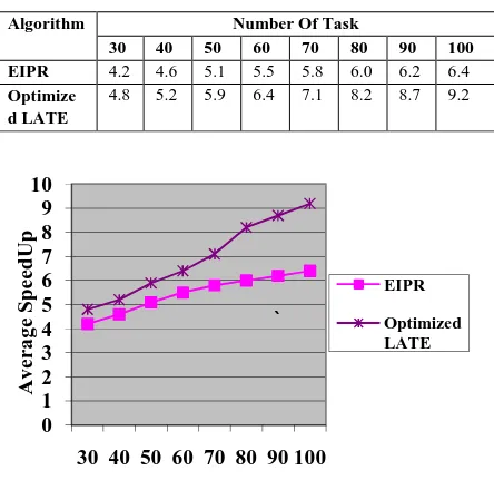
5.3.2 Speed Up: Speed up is the ratio of the sequential execution time to the parallel execution time. The given Table 5.2 and Figure 5.3 show Comparison of no of task vs Average Speed Up.
Table 5.2. Average Speed Up
Algorithm Number Of Task
30 40 50 60 70 80 90 100 EIPR 4.2 4.6 5.1 5.5 5.8 6.0 6.2 6.4 Optimize
d LATE
4.8 5.2 5.9 6.4 7.1 8.2 8.7 9.2
Fig 5.3. Comparison of no of task vs Averages
SpeedUp
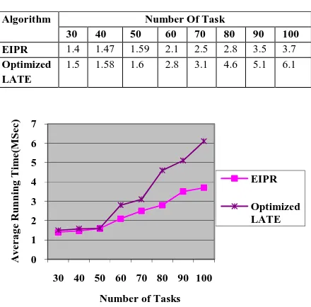
Table 5.3. Average Running Time
Fig 5.4. Comparison of no of task vs Average
Running Time
5.3.4 Performance Analysis of CPU Utilization (%) The LATE algorithm is used to number of virtual machines to calculate the CPU Utilization (%). The given Table 5.4 and Figure 5.5 show Comparison of number of Virtual Node vs CPU Utilization (%).
Table 5.4. CPU Utilization (%)
Algorithm Number of Virtual Machine 1 2 3 4
EIPR 81 67 61 52 48 Optimized
LATE
77 63 57 49 45
Fig 5.5. Comparison of no of Virtual Node vs CPU
Utilization (%)
Comparison of no of task vs Average
CPU Utilization (%):
The LATE algorithm is used to number of virtual machines to calculate the CPU Utilization (%). The 5.5 show Comparison of number of Virtual Node vs CPU Utilization (%).
CPU Utilization (%)
Number of Virtual Machine 5 6 7 8
48 42 39 36
45 37 34 28
Comparison of no of Virtual Node vs CPU
6. CONCLUSION
Motivated by the real
node heterogeneity, we have analyzed the problem of speculative execution in cloud. We identified flaws with both the particular threshold
algorithm in clouds and with progress
algorithms in general. We designed a simple, robust scheduling algorithm LATE, which uses estimated finish times to speculatively execute the tasks that hurt the response times the most. LATE perf significantly better than clouds default speculative execution algorithm in real workloads.
ACKNOWLEDGEMENTS
Mr. S.Vinodkumar, Assistant Professor, PG Department of Computer Science,
Saraswathi Thyagaraja College (Autonomous),
Pollachi, Coimbatore, Tamilnadu, India, for her excellent guidance, caring out this work. His research paper wouldn’t have been a success for me without his cooperation and valuable comments and suggestions. His understanding, encouraging and personal guidance have provided a good basis for the present research paper. computing. Technical Report UCB/EECS 28, EECS Department, University of California, Berkeley, Feb 2009.
[2] Barham, Paul and Dragovic, Boris and Fraser, Keir and Hand, Steven and Harris, Tim and Ho, Alex and Neugebauer, Ro
Warfield, Andrew. Xen and the art of virtualization. In SOSP ’03: Proceedings of the nineteenth ACM symposium on Operating systems principles, 2003, 1
177, Bolton Landing, NY, USA, Beloglazov, Cesar A. F. De Rose, and Rajkumar Buyya. CloudSim : A Toolk
Simulation of Cloud Computing Environments and Evaluation of Resource Provisioning
100 node heterogeneity, we have analyzed the problem of speculative execution in cloud. We identified flaws with both the particular threshold-based scheduling algorithm in clouds and with progress-rate-based algorithms in general. We designed a simple, robust scheduling algorithm LATE, which uses estimated finish times to speculatively execute the tasks that hurt the response times the most. LATE performs significantly better than clouds default speculative execution algorithm in real workloads.
ACKNOWLEDGEMENTS
Mr. S.Vinodkumar, Assistant Professor, PG Department of Computer Science, Sree
Saraswathi Thyagaraja College (Autonomous),
Coimbatore, Tamilnadu, India, for her excellent guidance, caring out this work. His research paper wouldn’t have been a success for me without his cooperation and valuable comments and suggestions. His understanding, encouraging and provided a good basis for the
[1] Michael Armbrust, Armando Fox, Rean Griffith, Anthony D. Joseph, Randy H.Katz, Andrew Konwinski, Gunho Lee, David A. Patterson, Ariel Rabkin, IonStoica, and Matei Zaharia. ds: A berkeley view of cloud computing. Technical Report UCB/EECS-2009-28, EECS Department, University of California,
[2] Barham, Paul and Dragovic, Boris and Fraser, Keir and Hand, Steven and Harris, Tim and Ho, Alex and Neugebauer, Rolf and Pratt, Ian and Warfield, Andrew. Xen and the art of virtualization. In SOSP ’03: Proceedings of the nineteenth ACM symposium on Operating systems principles, 2003, 1-58113-757-5, 164–
Algorithms. Software: Practice and Experience, ISSN: 0038-0644, Wiley Press, New York, USA, 2010 (in press, accepted on June 14, 2010). [5] Rajkumar Buyya, Rajiv Ranjan and Rodrigo N.
Calheiros. Modeling and Simulation of Scalable
Cloud Computing Environments and the
CloudSim Toolkit: Challenges and
Opportunities. In Proceedings of the 7th High
Performance Computing and Simulation
Conference (HPCS 2009, ISBN: 978-1-4244-4907-1, IEEE Press, New York, USA), Leipzig, Germany, June 21-24, 2009. [6] Sujesha
Sudevalayam and Purushottam Kulkarni.
Affinity-aware Modeling of CPU Usage for
Provisioning Virtualized Applications. In
Proceedings of IEEE Cloud 2011, the 4th
International Conference on Cloud Computing, Washington DC, USA.
[7] The BRITE Output Format. Website.
http://www.cs.bu.edu/brite/user/manual/node29. html
[8] G. Juve, A. Chervenak, E. Deelman, S. Bharathi, G. Mehta, and K. Vahi, ‘‘Characterizing and Profiling Scientific Workflows,’’ Future Gener. Comput. Syst., vol. 29, no. 3, pp. 682-692, Mar. 2013.
[9] R. Abbott and H. Garcia-Molina, ‘‘Scheduling Real-Time Transactions,’’ ACM SIGMOD Rec., vol. 17, no. 1, pp. 71-81, Mar. 1988.
[10] K.R. Jackson, L. Ramakrishnan,K.Muriki, S. Canon, S. Cholia, J. Shalf, H.J.Wasserman, and N.J.Wright, ‘‘Performance Analysis of High Performance Computing Applications on the Amazon Web Services Cloud,’’ in Proc. 2nd Int’l Conf. CloudCom, 2010,pp. 159-168. [11] Y.K. Kwok and I. Ahmad, ‘‘Static Scheduling
Algorithms for Allocating Directed Task Graphs to Multiprocessors,’’ ACM Comput. Surveys, vol. 31, no. 4, pp. 406-471, Dec. 1999.
[12] Z. Shi and J.J. Dongarra, ‘‘Scheduling Workflow Applications on Processors with Different Capabilities,’’ Future Gener. Comput. Syst., vol. 22, no. 6, pp. 665-675, May 2006.
[13] Rodrigo N. Calheiros
,
Rajkumar Buyya”
Meeting Deadlines of Scientific Workflows in
Public Clouds with Tasks Replication”, IEEE
TRANSACTIONS ON PARALLEL AND DISTRIBUTED SYSTEMS, VOL. 25, NO. 7, JULY 2014,pp.1787 -1796.
[14] A.Hirales-Carbajal, A. Tchernykh, R.
Yahyapour, J.L. Gonza´lez-Garcı´a, T. Ro¨ blitz,
and J.M. Ramı´rez-Alcaraz, ‘‘Multiple
Workflow Scheduling Strategies with User Run Time Estimates on a Grid,’’ J. Grid Comput., vol. 10, no. 2, pp. 325-346, June 2012.
[15] C. Lin and S. Lu, ‘‘SCPOR: An Elastic Workflow Scheduling Algorithm for Services Computing,’’ in Proc. Int’l Conf. SOCA, 2011, pp. 1-8.
[16] C.J.Reynolds, S.Winter, G.Z.Terstyanszky, T. Kiss,P.Greenwell, S. Acs, and P. Kacsuk, ‘‘Scientific Workflow Makespan Reduction through Cloud Augmented Desktop Grids,’’ in Proc. 3rd Int’l Conf. CloudCom, 2011, pp. 18- [17] M. Xu, L. Cui, H. Wang, and Y. Bi, ‘‘A
Multiple QoS Constrained Scheduling Strategy of Multiple Workflows for Cloud Computing,’’ in Proc. Int’l Symp. ISPA, 2009, pp. 629-634. [18] M. Mao and M. Humphrey, ‘‘Auto-Scaling to
Minimize Cost and Meet Application Deadlines in Cloud Workflows,’’ in Proc. Int’l Conf. High Perform. Comput., Netw., Storage Anal. (SC), 2011, p. 49.
[19] M. Rahman, X. Li, and H. Palit, ‘‘Hybrid
Heuristic for Scheduling Data Analytics
Workflow Applications in Hybrid Cloud Environment,’’ in Proc. IPDPSW, 2011, pp. 966-974.
[20] E.K. Byun, Y.S. Kee, J.S. Kim, and S. Maeng, ‘‘Cost Optimized Provisioning of Elastic Resources for Application Workflows,’’ Future Gener. Comput. Syst., vol. 27, no. 8, pp. 1011-1026,Oct. 2011.
[21] S. Abrishami, M. Naghibzadeh, and D. Epema, ‘‘Deadline- Constrained Workflow Scheduling Algorithms for IaaS Clouds,’’ Future Gener. Comput. Syst., vol. 29, no. 1, pp. 158-169, Jan. 2013.
[22] R. Sirvent, R.M. Badia, and J. Labarta,
‘‘Graph-Based Task Replication for Workflow
Applications,’’ in Proc. 11th Int’l Conf. HPCC, 2009, pp. 20-28.
[23] M. Dobber, R. van der Mei, and G. Koole, ‘‘Dynamic Load Balancing and Job Replication in a Global-Scale Grid Environment: A Comparison,’’ IEEE Trans. Parallel Distrib. Syst., vol. 20,no. 2, pp. 207-218, Feb. 2009. [24] X. Tang, K. Li, G. Liao, and R. Li, ‘‘List
Scheduling with Duplication for Heterogeneous Computing Systems,’’ J. Parallel Distrib. Comput., vol. 70, no. 4, pp. 323-329, Apr. 2010. [25] K. Plankensteiner and R. Prodan, ‘‘Meeting Soft
Deadlines in Scientific Workflows Using Resubmission Impact,’’ IEEE Trans. Parallel Distrib. Syst., vol. 23, no. 5, pp. 890-901, May 2012.
Distributed Environments,’’ in Proc. 8th Int’l Conf. E-Science, 2012, pp. 1-8.
[27] Matei Zaharia, Andy Konwinski, Anthony D. Joseph, Randy Katz, Ion Stoica, “Improving MapReduce Performance in Heterogeneous Environments” , USENIX Association, 8th USENIX Symposium on Operating Systems