Study on Impact of Sea Level Rise and Extreme Sea State on Coastal Inundation in Tamil Nadu

Study on Impact of Sea Level Rise and Extreme Sea State on Coastal

Inundation in Tamil Nadu

Hezron Philip J

_,

_{S. Jayalakshmi}

_,

1

_{M.E. Geomatics student, Institute of Remote Sensing, College of Engineering, Guindy, Anna University, Chennai,}

India.*Correspondence: jhezronphilip@gmail.com

2

_{Assistant Professor, Institute of Remote Sensing, College of Engineering, Guindy, Anna University, Chennai, India.}

GIS based inundation mapping is done on the digital elevation model to determine the areas that are vulnerable to the flooding. This is compared with the observed values of inundation due to the tsunami during the year 2004 to validate the model.

The model is used to map the inundation for the year 2100 and to assess the socio-economic impacts, as well as the comparative impact on the land use land cover of Tamil Nadu with respect to a hypothetical scenario of extreme conditions during the year 2012.

The Analysis of the affected land use gives us a clear picture as to the areas that are most affected by the projected inundation. The wetlands (86.27%) and the mangrove forests (96.86%) are the land uses that have

projected inundation. The districts worst affected by the projected inundation are Cuddalore, Nagapattinam and Rameswaram. This is due to the low elevation of these directly resulted in an increased rate of sea level rise due to a wide range of factors, the least of which is not the melting of polar ice caps. This increase in sea level impacts adversely on low lying coastal areas, where the increase in sea level creates a huge risk in coastal inundation. Any rise in the mean sea level will result in the retreat of unprotected coastlines due to coastal inundation, erosion and increased storm flooding. As emphasized in the Fourth Assessment Report of the Intergovernmental Panel on Climate Change (2007), the global sea level rose by 1.8 to 3.1 mm/year during the last century and present estimates of future rise range from 18 cm to 59 cm by the year 2100. Low lying areas such as beach ridges, coastal plains, deltas, estuaries, lagoons, and bays would be the areas that would suffer the most as a result of the enhanced sea level rise.

level rise on gross domestic product (GDP) is slightly greater than the impact on population, because GDP per capita is generally above average for coastal populations and cities.

Since the start of the Industrial Revolution the focus has been on economic development rather than environmental sustainability. By estimating the coastal inundation, we can assess the damage and impacts at the social and economic levels. One of the most likely consequences of global warming is an accelerated Sea-Level Rise (SLR) mainly due to oceanic thermal expansion and melting of glaciers, Greenland and Antarctic ice sheets. Comparison of the rate of SLR over the last two millennia indicates a relatively recent acceleration in the rate of SLR in the last century. According to IPCC Third Assessment Report (2001), the global SLR in the 20th century was 10 to 20 cm and predicted that a further accelerated rise of 9-88 cm will occur between 1990 and 2100 with a mid-estimate of 48 cm. This faster rate of the SLR mid-estimated at 1-2 mm per year is caused by human-induced global warming. Whereas, IPCC Fourth Assessment Report (2007) projected a global SLR of 18-59 cm from 1990 to the 2090s. These ranges are narrower than in the Third Assessment Report (2001), mainly because of improved information about some uncertainties in the projected contributions. However, the global mean SLR will not be uniform around the world since the local change in sea level at any coastal location depends on the sum of global, regional, and local factors, which is termed as relative sea level change.

Relative SLR is a major factor contributing to recent losses and projected future reductions in the area of valued coastal habitats, including mangroves and other tidal wetlands, with an increased threat to human safety and shoreline development from coastal. Many of the world’s coastal wetlands have suffered significant losses during this century. This is a concern because they provide valuable services, such as flood protection and fisheries production, for a global human population that is increasingly concentrated near the coast and dependent on its resources. Moreover, the direct effect of inundation is the potential large loss of inhabited areas, particularly in low-lying, flat deltaic and estuarine areas. Half of humanity inhabits the coastal regions around the globe, and large areas of highly vulnerable flood prone sections are densely populated.

On the other hand, the response of coastal ecosystems to climate change and SLR is strongly influenced by continuing developments, i.e. Developments that in many cases lead to overexploitation of resources, pollution, sediment starvation and fragmentation of ecosystems through urbanization and development of infrastructure. These developments will, on an increasing scale: lead to a decrease in the resilience of coastal systems in coping with natural climate variability; adversely affect the natural capability of the systems to adapt to changes in climate; lead to the increased hazard potential for the coastal population, infrastructure and investments, therefore, the assessment of impacts of climate change in coastal areas involves the estimation of the additional risk that is posed by climate change to systems that already are under significant stress. Thus, predictions of changes in coastal ecosystem boundaries, in response to projected relative SLR, enables advanced planning appropriate for specific sections of coastline to minimize and offset anticipated losses and reduce threats to coastal development and human safety. The objective of this study is to identify and quantify the coastal dependent social communities to the adverse impact of SLR and extreme sea state using GIS and to mainstream, the importance of coastal adaptation to the inundation of the coast.

2. DESCRIPTION OF THE STUDY AREA

The study area comprises of Tamil Nadu which is part of the Indian Peninsula that has a coastline of 1076km which accounts for 15% of the Indian Coast. The study area is outlined in figure 1. Changes in the coastline due to the afore mentioned factors will lead to loss of the coastal lands over the prolonged duration and have a socio-economic impact even with regard to India’s strict coastal regulations . Therefore, it is necessary to study these changes and the impacts they pose on the coastline.

3. METHODOLOGY

Figure 2:

3.1 ESTIMATION OF INUNDATION LEVEL

The first step involved in the process is the estimation of the inundation level. This is done by using the risk zone definition of Hoozemans et al. (1993) where the inundation level (Inlev) is given by Eq. (1), i.e. the sum of

mean high water (MHW), relative sea level rise (S), extreme wave height (HTR) and sea level change due to the

barometric pressure (SP)

..(1)

MHW is defined as the average of all the high water heights above the mean sea surface observed during the altimetry data period from 1992 to 2014. It is calculated using Eq. (2).

..(2)

The current rate of sea level rise has been determined using Eq. (3), that includes bias and trend that is given by:

..(3)

where t is time, t0 is the origin of time or reference epoch,

SLA(t0) is the initial sea level anomaly at time t=t0, A1 is a

constant rate of sea level rise and ε(t) is the error term. The unknown parameters in Eq. (3) are derived by fitting the least squares regression to the altimetric sea level time series. Assuming there are no significant land movements (subsidence/ uplift) in the vicinity of the study, no

acceleration in the rate of sea level rise, and no inter annual to decadal changes in the seasonal parameters. The relative sea level rise S is projected for 2004 and 2100 using the estimated parameters of the above harmonic model.

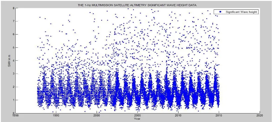
The extreme significant wave height with a return period of 100 years has been predicted using Gumbel extreme value distribution. According to this statistical distribution, the wave height expected for a selected return period HTR can be estimated using Eq. (4).

..(4)

Where α and β represent the location and scale parameters, respectively, and P is the probability of non-exceedance. The model is fitted to the cumulative distribution function (CDF) of the altimetric wave data, which have been constructed using Eq. (5).

..(5)

Where m is the rank based on descending order of magnitude and N is the total number of passes or data points within the study area. The extreme wave height with a 100-year return period (H100) has been predicted from the estimated parameters of the distribution model and the non-exceedance probability given by Eq. (6), where D is the de-correlation time scale in hours for significant wave height (SWH) observations (3 h), and

P( ..(6)

The term SP is computed from the MOG2D (2D Gravity

Waves) model. The model is used in the satellite altimetry data processing to account for the high frequency sea level variations caused by pressure and wind forcing. The extreme meteorological contribution to sea level is considered in this study. Therefore, the term SP is computed exactly in the same way as is done for MHW, where the highest values over each satellite repeat cycle and pass are averaged as shown in Eq. (7).

..(7)

The “eight-side rule” approach used by Rodriguez (2010) is used to simulate inundation in this study. A grid cell of the digital elevation model (DEM) is flooded only if its elevation is below the inundation level and if it is connected to an adjacent grid cell that is flooded or open water. Therefore, the surface connectivity between a grid cell and its immediate 8 neighbours in the cardinal and

Inundation Mapping and analysis of flooding impacts require data on the land surface elevations, land use and cover. The DEM for the study area was acquired from the freely available SRTM DEM data. The raster grid containing the elevation information was stored as a TIFF file for further processing. The land use land cover map for the study area was prepared using the LISS III satellite imagery acquired for the year 2012 by means of image classification on the ERDAS platform. The satellite imagery corrected and registered as a geoTIFF with 23.5 m resolution. Supervised classification is done using the maximum likelihood classifier based on training signatures established by onscreen digitization of the false colour composite based on the land use land cover of Tamil Nadu (2011-2012) obtained from Google Earth images and Google Maps. Finally the classified image is converted into vector format for further analysis.

4. ANALYSIS AND RESULTS

4.1

Satellite Altimetry Data and Inundation Level

The mean high water level, the rate of the mean sea level rise, and the extreme wave height with a return period of

100 years has been computed based on the sea level anomaly (SLA) and SWH data of Topex, Poseidon, Jason-1 and Jason-2 altimeter satellites. The standard along-track altimetry data from the Radar Altimetry Data System (RADS) is extracted for the study area using version 3.1 of the default settings in the RADS database as described by Scharroo (2011). SLA and SWH time series cover Topex cycles 1 to 364 (October 1992 to August 2002), Jason-1 cycles 1 to 260 (January 2002 to January 2009), and Jason-2 cycles 1 to Jason-239 (July Jason-2008 to January Jason-2015), each having average repeat cycles of 9.9 days. Default data editing criteria (limits and flags) have been accepted during the SLA and SWH data construction. The sea level anomalies are given with respect to the DNSC08 global mean sea surface model derived from a combination of 12 years of satellite altimetry from 8 different satellites covering the period of 1993–2004.

4.1.1 Mean High Water

The MHW level was estimated using the SLA data from the RADS database from which the tidal corrections have been removed was used. The highest values for each satellite repeat cycle and pass is averaged to estimate the MHW [Eq. (2)]. The MHW is found to be 17 cm above the mean sea surface for the year 2004.

4.1.2 Relative Sea Level Rise

The rate of sea level rise and sea level variations are obtained from the multi-mission RADAR altimetry satellites such as the Topex/Poseidon, 1 and Jason-2. The variation in the MSL over the period from January 1993 to June 2014 is plotted and a mean sea level rise of 3.43 mm/year superimposed to the seasonal variations is observed from figure 3. This is consistent with the regional and global estimates. Projection suggests that the mean sea level had risen up to 3.233 cm in 2004 with respect to the MSL in 2000, which is also consistent with global mean sea level rise scenarios of IPCC Fourth Annual Report(2007).

4.1.3 Sea Level Changes due to Barometric

Pressure

Figure 3: Smoothed mean sea level signal from January 1993 to June 2014, and the rate of sea level rise

4.1.4 Extreme Wave Height

Multi-mission satellite altimetry (figure 4) is used for the prediction of the 100-year return wave height. The median of the SWH data over each satellite repeat cycle is computed and the data is used to describe the empirical CDF, or probability, of non-exceedance of wave height [Eq. 5]. The SWH is then plotted against the reduced variate of Gumbel distribution -In[In(1/P)] and is fitted to obtain the parameters of the probability distribution (Figures 5 and

6). The non-exceedance probability of H100 [Eq. (6)] and

the estimated parameters of probability distribution are used to determine the extreme wave height for a return period of 100 years [Eq. 4]. The location and scale parameters of the Gumbel distribution are 0.6436 and 0.2611. The non-exceedance probability is 0.999996582. These values can be used to determine the predicted value of H100. The extreme wave height as predicted by this

equation for the year 2004 is 3.089 m.

Figure 5:

Figure 6:

4.2 Inundation Mapping

The computation for the projected inundation level in extreme conditions for the year 2004 is obtained as 3.64 m. This value is then applied to the SRTM DEM raster by using the Raster Calculator tool to reduce the raster to the inundation level. This new raster can now be run through a conditional statement to create a binary raster that shows the inundated areas. The binary raster has to be processed such that only the connected pixels, i.e., the pixels that are connected to open water are flooded. This can be done by using the “bwconncomp” function in MATLAB. The output image is now exported to ArcGIS and converted to a feature layer (Polygon) for further analysis.

5. Validation

Validation is done by comparing the projections for the year 2004 to the actual observed values of inundation on

the aftermath of one of the most extreme conditions to affect the Tamil Nadu coast, the Tsunami of December 2004. In order to validate the Inundation Map for the year 2004 (Figure 8) with respect to the modeled value of 3.64 m, the observed inundation at 50 points during the aftermath of the Tsunami in Chennai and its surrounding areas was used (Satheesh Kumar et. al., 2008).

The validation process was carried out by plotting the observed values of inundation against the modelled values of inundation (Figure 7); the plot has a fit with an R-square value of 0.9103 and provides proof that the modelled inundation for the year 2004 provides an accurate representation of the observed inundation during the same period. Therefore the modeled inundation for the year 2100 can be used to analyze the impacts it will have on the study area.

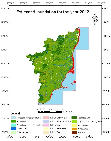
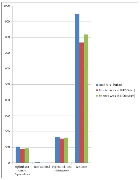
6. RESULTS AND ANALYSIS indicates that with the projected inundation 3.96 m for the year 2012, about 2.2% of the total area of Tamil Nadu will be at a risk of flooding; this translates to roughly 2855.72 sqkm along the coast of Tamil Nadu. Overlaying the inundated areas and land use map shows that about 1.59% of the agricultural land, 86.1% of aquaculture farms, 1.7% of the Built Up area, 93.32% of the Mangrove vegetated area, 1.63% of the wastelands and 80.9% of the wetlands would be exposed to permanent as well as temporary inundation.

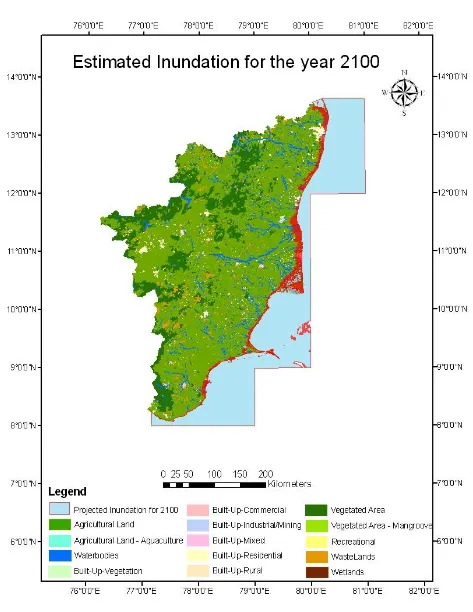
The inundation for the year 2100 is found to be 4.81 m and this inundation height is applied to the digital elevation model and the inundation map is prepared. This inundation map is overlaid on the 2012 land use land cover map assuming the land use conditions remain the same in 2100 so that the amount of damage that will be caused by the extreme conditions can be assessed

The inundation map presented in Figure 10 indicates that with the projected inundation 4.81 m for the year 2100, about 2.81% of the total area of Tamil Nadu will be at a risk of flooding; this translates to roughly 3658.18 sqkm along the coast of Tamil Nadu. Overlaying the inundated areas and land use map shows that about 2.26% of the agricultural land, 90.78% of aquaculture farms, 2.59% of the Built Up area, 96.86% of the Mangrove vegetated area, 2.08% of the wastelands and 86.27% of the wetlands would be exposed to permanent as well as temporary inundation.

Population and GDP per capita of the state of Tamil Nadu were obtained from the information available in the Census of India website. The population was forecast for 2100 using the Logistic Curve Method.

Table 1 and table 2 provide the results of the comparative analysis of the coastal vulnerability of Tamil Nadu to inundation in the year 2012, based on a computed inundation height of 3.96 m; and the vulnerability of the Tamil Nadu coast for the year 2100 assuming similar land use to the 2012 scenario.

The results of the analysis show us that the land uses that are most affected by the Inundation are the Mangroves and the Wetlands. The wetlands of Kodiakarai Wildlife and Bird Sanctuary, otherwise known as Point Calimere, is a low headland on the Coromandel Coast, in Nagapattinam district and the wetlands of Natarajapuram near Rameshwaram lying between 9.2° N and 9.3° N are some of the worst affected by the projected inundation.

The Mangrove forest of Muthupet, also found in the Kodiakarai Wildlife and Bird Sanctuary in Nagapattinam District accounts for a major part of the Mangrove vegetation affected by the projected Inundation.

7. CONCLUSION

The result obtained in this study shows that the rise in the sea level severely affects the coastal land use. The sea level rise is modeled using four parameters, i.e., mean high water, relative sea level rise, extreme wave height and changes in sea level due to barometric pressure. Thus the Sea level rise modeling for the extreme sea state scenario shows that the maximum height of the inundation is 3.64 m for the year 2004, which is validated using the inundation data that was observed during the 2004 tsunami. Thus, the model is used to predict the inundation for the year 2100 i.e. 4.81 m. The estimated height of inundation can be applied to the coast in order to determine the impacts it has, by using the Digital Elevation Model.

The model is used to create a worst case scenario thereby projects the worst possible effects sea level rise can have on the coast of Tamil Nadu. The main objective of the study is to determine the land use and land cover that is affected by the sea level rise. It is also used to estimate the Socio-Economic impact of the sea level rise on Tamil Nadu.

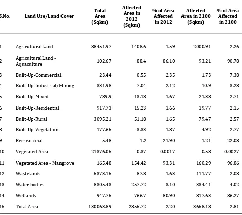
Table 1

S.No. Land Use/Land Cover

Total Area (Sqkm)

Affected Area in

2012 (Sqkm)

% of Area Affected

in 2012

Affected Area in 2100

(Sqkm)

% of Area Affected

in 2100

1 Agricultural Land 88451.97 1408.6 1.59 2000.91 2.26

2 Agricultural Land -

Aquaculture 102.67 88.4 86.10 93.21 90.78

3 Built-Up-Commercial 23.44 0.55 2.35 1.73 7.38

4 Built-Up-Industrial/Mining 331.98 7.04 2.12 10.9 3.28

5 Built-Up-Mixed 789.9 13.18 1.67 21.38 2.71

6 Built-Up-Residential 917.73 15.23 1.66 19.77 2.15

7 Built-Up-Rural 3095.21 51.18 1.65 79.47 2.57

8 Built-Up-Vegetation 177.65 3.33 1.87 4.92 2.77

9 Recreational 5.48 1.2 21.90 1.21 22.08

10 Vegetated Area 21376.05 0.37 0.0017 0.58 0.0027

11 Vegetated Area - Mangrove 165.48 154.42 93.31 160.29 96.86

12 Wastelands 5373.15 87.8 1.63 111.77 2.08

13 Water bodies 8305.43 257.72 3.10 334.41 4.02

14 Wetlands 947.75 766.7 80.90 817.63 86.27

15 Total Area 130063.89 2855.72 2.20 3658.18 2.81

Table 2

S.No. _{Description Unit Affected by Inundation}

1 Population in 2012 554.34 people/km2 _1,583,039

2 GDP for 2012 $1622 per capita $2,567,689,258

3 Population in 2100 691.54 people/km2 _2,529,763

References

Dasgupta, S., Laplante, B., Meisner, C., Wheeler, D. and Yan, J. 2007. The Impact of Sea Level Rise on developing countries: A comparative analysis. World Bank Policy

Research Working paper, 4136.

Available at http://econ.worldbank.org.

Hoozemans, F.M.J., Marchand, M, and Pennekamp, H.A. 1993. Sea level Rise: A Global Vulnerability Assessment-Vulnerability Assessments for population, Coastal Wetlands and Rice Producation on a Global Scale, 2nd _ed. Delft Hydraulics, Delft, The Netherlands.

James J. McCarthy, Osvaldo F. Canziani, Niel A. Leary, David J. Dokken, and Kasey S. White, 2001, Working Group II: Impacts Adaptation and Vulnerability, IPCC Third

Assessment Report: Climate Change 2001.

Ozlem Simav, Dursun Zafer Seker, Cem Gazioglu, 2013. Coastal Inundation due to sea level rise and extreme sea state and its potential impacts: Cukurova Delta Case.

Turkish Journal of Earth Sciences (2013) 22:671-680.

Parry M.L., O.F. Canziani, J.P. Palutikof, P.J. van der Linden and C.E. Hanson, 2007, Contribution of Working Group II to the Fourth Assessment Report of the Intergovernmental Panel on Climate Change, 2007 Cambridge University Press, Cambridge, United Kingdom and New York, NY, USA.

Rodriguez A., 2010, Mexican Gulf of Mexico regional introduction and sea level rise analysis of the Carmen

Island, Campeche, Mexico.

http://www.geo.utexas.edu/courses/371c/projects/Rodri guez.pdf

Saleem Khan A., A. Ramachandran, N. Usha, S. Punitha, V. Selvam, 2012, Predicted impact of sea level rise at Vellar-Coleroon estuarine region of Tamil Nadu Coast in India: Mainstreaming adaptation as a coastal zone management option. Ocean & Coastal Management 69 (2012) 327e339.

Satheesh Kumar C., P. Arul Murugan, R. R. Krishnamurthy, B. Prabhu Doss Batvari, M. V. Ramanamurthy, T. Usha, and Y. Pari, Inundation Mapping – A Study Based On December 2004 Tsunami Hazard Along Chennai Coast, Southeast India.