Spectrum efficiency of nested sparse sampling and coprime sampling

R E S E A R C H

Open Access

Spectrum efficiency of nested sparse sampling

and coprime sampling

Junjie Chen

, Qilian Liang

, Baoju Zhang

and Xiaorong Wu

Abstract

This article addresses the spectrum efficiency study of nested sparse sampling and coprime sampling in the estimation of power spectral density for QPSK signal. The authors proposed nested sampling and coprime sampling only showed that these new sub-Nyquist sampling algorithm could achieve enhanced degrees of freedom, but did not consider its spectrum efficiency performance. Spectral efficiency describes the ability of a communication system to accommodate data within a limited bandwidth. In this article, we give the procedures of using nested and coprime sampling structure to estimate the QPSK signal’s autocorrelation and power spectral density (PSD) using a set of sparse samples. We also provide detailed theoretical analysis of the PSD of these two sampling algorithms with the increase of sampling intervals. Our results prove that the mainlobe of PSD becomes narrower as the sampling intervals increase for both nested and coprime sampling. Our simulation results also show that by making the sampling intervals, i.e.,N1 andN2for nested sampling, andPandQfor coprime sampling, large enough, the main lobe of PSD obtained from these two sub-Nyquist samplings are much narrower than the original QPSK signal. That is, the bandwidthB

occupancy of the sampled signal is smaller, which improves the spectrum efficiency. Besides the smaller average rate, the enhanced spectrum efficiency is a new advantage of both nested sparse sampling and coprime sampling.

Keywords: Spectrum efficiency, Nested sampling, Coprime sampling, Autocorrelation, Power spectral density

1 Introduction

In recent years, spectrum efficiency has gained renewed interest in wireless communication system. From [1], we know that the performance of a particular communication system is often measured in terms of spectral efficiency (or bandwidth efficiency). Spectral efficiency describes the ability of a communication system to accommodate data within a limited bandwidth. It reflects how efficiently the allocated bandwidth is utilized and defined as the ratio of the throughput data rate per Hertz in a given band-width. LettingRto be the data rate in bits per second, and Bthe bandwidth occupied, the bandwidth efficiencyηis expressed as

η= R

Bbit/s/Hz (1)

If we apply Shannon’s capacity to AWGN non-fading channel, i.e.,C =Blog₂(1+_NS), and with the knowledge

*Correspondence: [email protected]

1Department of Electrical Engineering, University of Texas at Arlington, Arlington, TX 76019-0016, USA

Full list of author information is available at the end of the article

that all communication rates are below channel capacity R ≤ C[2], we can get the fundamental upper bound [1] on achievable spectrum efficiency, for an arbitrarily small probability of error, where _NS is the signal to noise ratio.

ηmax=

C B =log2

1+ S N

(2)

From (1), if we hope to improve the spectrum efficiency, we should either increase the data rate R or efficiently use the bandwidthB. Lots of efforts have been made to increase the spectrum efficiency. For example, power and spectral efficient family of modulations for wireless com-munication systems were introduced in [3]. The author in [4] proposed a high spectrum efficient multiple access code. Cognitive radios have been proposed as a method to efficiently reuse the licensed limited spectrum. And in general, the spectral efficiency can be improved [5] by frequency re-use, spatial multiplexing, OFDMA, or some radio resource management techniques such as effi-cient fixed or dynamic channel allocation, power control, link adaptation etc. As stated in [6], time is also a fac-tor in determining overall spectrum efficiency, because

most applications do not use spectrum on a continu-ous basis and users typically share resources on a time basis.

A new approach to super resolution spectral estimation using nested sparse sampling is provided by [7,8]. In [8], a two user case of sparse sampling, coprime sampling is also introduced. The authors has already proved that these two new sub-Nyquist sampling algorithms could achieve enhanced degrees of freedom. While in this article, we will show that both nested sparse sampling and coprime sam-pling are much more spectrum efficiency, i.e., they occupy much narrower bandwidth than the original non-sampled signal.

Traditional sampling methods are based on Nyquist rate sampling, which will have poor efficiency in terms of both sampling rate and computational complexity. Nowadays, more and more techniques are proposed to overcome the Nyquist sampling. Compressive sensing [9] provides us a new point of view, which could only use much less samples to perfectly recover the original signal at a high com-pression ratio. The authors give a new idea of coprime sampling in [8], which uses two uniform sampling to estimate the autocorrelation for all lags.

Differently, nested sparse sampling is an non-uniform sampling, using two different samplers in each period. Although the signal is sampled sparsely and nonuniformly at 1 ≤ l ≤ N1T and(N1+1)mT,1 ≤ m ≤ N2for one period, the autocorrelationRc(τ )of the signalxc(t)could

be estimated at all lagsτ =kT,k,l, andmare all integers. Hence, nested sparse sampling can be used to estimate power spectrum even though the samples in the time domain can be arbitrarily sparse [8]. While coprime sam-pling uses two uniform samplers, with sample spacings PTandQT, respectively, wherePandQare coprime inte-gers. Similar as nested sparse sampling case, the authors in [8] proved that the estimates of all lags of autocorrelation Rc(kT)could be obtained from these two sets of samples

of the signalxc(t), both of the samples are taken at much

smaller rates than Nyquist sampling rate, which results in a much less time consumption.

In this article, we give the principle of nested sparse sampling and coprime sampling first and provide the pro-cedures of using these two sparse sampling structures to estimate the QPSK signal’s autocorrelation and power spectral density (PSD). We give the theoretical analysis of how these two sparse sampling methods effect the power spectral density as well. Our simulation results also show that with if we choose the sampling spacings larger, the main lobe of PSD obtained from these two sampling will be much narrower than the original QPSK signal. That is, besides the much less time consumption, the occupied bandwidthBin expression (1) is smaller, which makes the spectrum efficiency higher. Besides the smaller average rate, the increased spectrum efficiency is a new advantage

of these two sparse sampling algorithms, which is studied for the first time.

The rest of this article is organized as follows. In Section 2, we give a brief overview of nested sparse sampling. An introduction of coprime sampling is in Section 3. Spectrum estimation based on the difference sets obtained from both nested sampling and coprime sampling structures is detailed in Section 4. In Section 5, we give the theoretical analysis of these two sparse sam-pling and how they will effect the power spectral den-sity. In Section 6, we provide the numerical results of the power spectral density estimation. Conclusions are presented in Section 7.

2 Nested sparse sampling

The nested array was introduced in [7] as an effective approach to array processing with enhanced degrees of freedom [10]. The time domain autocorrelation could also be obtained from sparse sampling with nested sampling structure [11]. And the samples of the autocorrelation can be computed at any specified rate, although the sam-ples from this nested sparse sampling are sparsely and nonuniformly located.

In the simplest form, the nested array [11] has two lev-els of sampling density, with the level 1 samples at theN1 locations and the level 2 samples at theN2locations.

1≤l≤N1, for level 1

(N1+1)m, 1≤m≤N2, for level 2

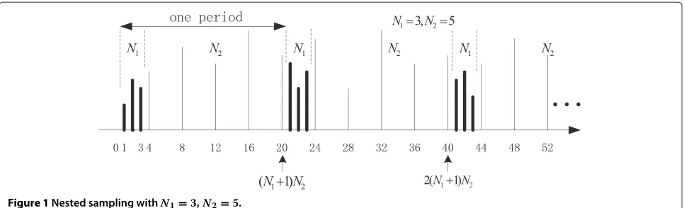
Figure 1 shows an example of periodic sparse sampling using nested sampling structure withN1=3 andN2=5. The cross-differences are given by

k=(N1+1)m−l, 1≤m≤N2, 1≤l≤N1 (3)

The cross-differences [11] are in the following range with the maximum value(N1+1)N2−1, except the integers and the corresponding negated versions shown in (5).

−[(N1+1)N2−1]≤k≤[(N1+1)N2−1] (4)

(N1+1), 2(N1+1),. . .,(N2−1)(N1+1) (5)

For example, consider the example in Figure 1, where 1 ≤ m ≤ 5 and 1 ≤ l ≤ 3, the cross differences k = (N1+1)m−lwill achieve these values

1, 2, 3,(), 5, 6, 7,(), 9, 10, 11,(), 13, 14, 15,(), 17, 18, 19

with 4, 8, 12, 16 missing.

Besides these integers, the difference 0 is also missing, for the reason thatmandlare nonzero. While, we notice that the self differences among the second array could cover all of the missing differences, as shown

Figure 1Nested sampling withN1=3,N2=5.

The difference-co-array could be obtained from the cross-differences and the self-differences, which is a filled difference co-array as shown in (4). This means that using nested array structure, with sparse samples, we could obtain the degrees of freedom as

2[(N1+1)N2−1]+1=2(N1+1)N2−1 (7)

Using the above principle, we could get a sparse sampling using nested sampling structure as shown in Figure 1. We have two levels of nesting, with N1 level-1 samples and N2 level-2 samples in each period, with period (N1+ 1)N2. This shows that nested sampling is non-uniform and the samples obtained are very sparse.

Therefore, in(N1+1)N2Tseconds, there are totallyN1+

N2samples. The average sampling rate is

fs,nested= frequency, which is greater than twice of the maximum frequency. As the Nyquist sampling rate is 1/T, the aver-age sampling rate of nested sampling is smaller than the conventional Nyquist sampling rate.

If we set N1 and N2 larger, the average sampling rate

fs would be arbitrarily smaller. In the theoretical and

numerical results sections, we will show that withN1and

N2 becoming larger, the bandwidth of the power spec-trum density goes narrower, i.e., the specspec-trum gets more efficiently used.

3 Coprime sampling

Different with nested sampling, coprime sampling involves two sets of uniformly spaced samplers as shown in Figure 2.

The coprime sampling uniformly sample the wide-sense stationary (WSS) process xc(t) using two sub-Nyquist

samplers, with sample spacingPT andQT, respectively, wherePandQare coprime integers withP <Q. 1/THz

is the Nyquist rate for a bandlimited process, i.e., 1/T = 2fmax,fmaxbeing the highest frequency.

x(n)=xc(nT) (9)

Consider the product

x(Pn1)x∗(Qn2) (10)

where x(Pn1) andx(Qn2) comes from the first and the second sampler. Set the difference as

k=Pn1−Qn2 (11)

The authors in [11] have shown thatk can achieve any integer value in the range 0≤k≤PQ−1, ifn1andn2in the ranges 0≤n1≤2Q−1 and 0≤n2≤P−1.

For coprime sampling, the two samplers collectP+Q samples inPQTseconds, the average sampling rate is

fs,coprime= Nyquist sampling frequency. We could notice the average sampling rate of coprime sampling is much smaller than the conventional Nyquist sampling rate of 1/T.

Similar as stated in nested sampling, if we set P and Q larger, the average sampling rate would be arbitrar-ily smaller. We will show that with P andQ becoming larger, the bandwidth of the power spectrum density goes narrower.

4 Power spectral density estimation based on nested & coprime sampling

In this part, we will detail the estimation of PSD using nested and coprime sampling structure. In signal and sys-tems analysis, the autocorrelation plays a very important role. The autocorrelation function of a random signal describes the general dependence of the values of the sam-ples at one time on the values of the samsam-ples at another time.

The autocorrelation [12] of a real and stationary signal xc(t)is defined by this averaging

Rc(τ )=E[xc(t)x∗c(t−τ )] (13)

Rc(τ )is always real-valued and an even function with a

maximum value atτ =0.

For sampled signal, define x(n) = xc(nT), for some

fixed spacingT. For the autocorrelation samples,R(k) = Rc(kT), whereRc(·)as shown in (13). Therefore,

R(k)=E[xc(nT)x∗c((n−k)T)]=E[x(n)x∗(n−k)]

(14)

R(k) can be computed from samples of xc(t) taken at

an arbitrarily lower rate using nested or coprime sparse sampling.

And here we only list some important autocorrelation properties which will be used in this article:

(1) Maximum value: The magnitude of the autocorrelation function of a wide sense stationary random process at lagm is not greater than its value at lagm=0, i.e.,

R(0)≥|R(k)|,k=0 (15)

(2) The autocorrelation function of a periodic signal is also periodic.

(3) The autocorrelation function of WSS process is a conjugate symmetric function ofk :

R(k)=R∗(−k) (16)

The power spectral density (PSD) describes how the power of a signal or time series is distributed with fre-quency. The PSD is the Fourier transform of the autocor-relation function of the signal if the signal is treated as a wide-sense stationary random process [13]. Therefore, the Fourier transform ofRc(τ )is the PSDS(f),

S(f)=

∞

−∞Rc(τ )e

−2πifτ_{dτ (17)}

S(f) is a real-valued, nonnegative function. Definition (17) shows that S(−f) = S(f), i.e., the PSD is an even function of frequencyf.

Taking discrete Fourier transform (DFT) of these lags of autocorrelation values, we could obtain the power spectral density as

Next, we will separately describe how nested sam-pling and coprime samsam-pling estimate the autocorrelation function.

4.1 For nested sampling

For the samples obtained from nested sparse sampling, consider the productx(n1)x∗(n2), withn1andn2belong to the first period in Figure 1. We will get the samples at the following locations

1, 2,. . .,N1,(N1+1), 2(N1+1),. . .,N2(N1+1) (19)

The set of differencesn1−n2are exactly the difference-co-array described in (4), that is,n1−n2will achieve all integer values in (4).

We can see that although the signal is sampled sparsely and nonuniformly at 1≤l≤N1and(N1+1)m, 1≤m≤

N2for one period, the autocorrelationRc(τ )of the signal xc(t)could be estimated at all lagsτ =k.

An estimate of the autocorrelation samples for all k could be obtained [11] by averaging the products x(n1)x∗(n2)overLperiods,

4.2 For coprime sampling

As PandQare coprime, there exist integers 0 ≤ n1 ≤ 2Q−1 and 0 ≤ n2 ≤ P−1, such that the difference in Equation (11) can achieve any integer valuek=Pn1−Qn2 in the range of 0≤k≤PQ−1. Sincek =P(n1+Ql)−

Q(n2+Pl)for anyl, we can averagelto obtain an estimate of the autocorrelationR(k), that is,

ˆ

As nested sampling and coprime sampling are similar, in this part, I will use nested sparse sampling to state the theoretical analysis.

From the property of DFT, we know that, ifRˆ(k)are real, thenS(N−n)andS(n) are related by

S(N−n)= ¯S(n) (22)

0 20 40 60 80 100 −50

−40 −30 −20 −10 0 10 20 30 40 50

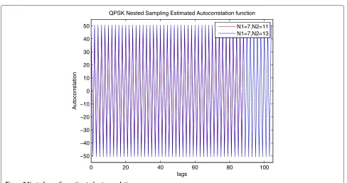
QPSK Nested Sampling Estimated Autocorrelation function

lags

Autocorrelation

N1=7,N2=11 N1=7,N2=13

Figure 3Nested sampling estimated autocorrelation.

In our simulation, we always consider the amplitude of the PSD, which indicates that

|S(N−n)| = |¯S(n)| (23)

This gives the reason of why the PSD figure is always symmetric.

From the simulation, we observe the absolute values of the autocorrelationRˆ(k)are the same for the QPSK signal,

which obtain positive or negative of a fixed value as shown in Figure 3 for differentN1andN2of nested sampling, and Figure 4 for differentPandQof coprime sampling. This could make the calculation of the PSD easier. In our anal-ysis, for simplicity, we assume all theRˆ(k)have the same absolute valueR, i.e., R = | ˆR(k)| = ˆR(0) = − ˆR(1) =

ˆ

R(2) = · · ·. Therefore, we setRˆ(k) = (−1)kR. The esti-mated autocorrelation satisfies those properties we stated

0 50 100 150

−50 −40 −30 −20 −10 0 10 20 30 40 50

QPSK Coprime Estimated Autocorrelation function

lags

Autocorrelation

P=7,Q=13 P=11,Q=13

before, i.e., Rˆ(0) ≥ | ˆR(k)|,k = 0, and as the QPSK signal we used is periodic, the estimated autocorrelation functionRˆ(k)is also periodic.

Let’s see how the PSD changes with the increase of N1 and N2. As stated in the principle of nested sparse sampling, k falls in the range of (4). Here we only use those positive, i.e., k = 0, 1,. . .,(N1 + 1)N2 − 1, that is, N = (N1 + 1)N2. We could get the PSD by taking the Fourier transform of the estimated autocorrelation,

As stated in the principle of nested sparse sampling,k falls in the range of (4),N = (N1+1)N2. For coprime

The corresponding amplitude of the PSD is

|S(n)| =R

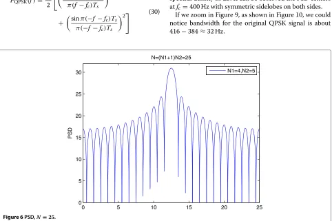
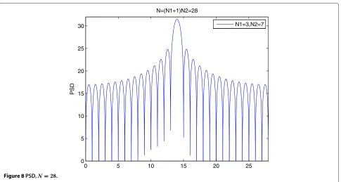
We could draw these two expressions in (27) as shown in Figures 5, 6, 7, and 8. It’s obvious that no matterNis odd or even, with the increase ofN, the mainlobe becomes narrower and the number of sidelobes increases. In next paragraph, we will prove the central of the mainlobe represents the central frequency.

In the simulation, if we takeN-point fast Fourier trans-form (FFT), we will get N PSD values. Letfnrepresents

the Nyquist sampling frequency,fn = 2fc (fcis the

car-rier frequency), usingf = fn·(0 : N −1)/N, we could

map these PSD values to the frequency. It is obvious that whenn = N/2, the PSD gets its central value ofS(N₂)at

From this derivation, we also notice that with the increase of N, besides the mainlobe becomes narrower, the central value of the PSD gets higher, which results in a higher spectrum efficiency.

In the numerical results part, we will show that with the same sampling spacings chosen for both nested and coprime sampling, i.e.,N1=P,N2=Q, we could achieve

N = (N1+1)N2for nested sampling will be larger than that ofN=PQfor coprime sampling, which will result in a better spectrum efficiency for nested sampling.

6 Numerical results

This section presents some numerical results for the auto-correlation and power spectrum density estimation using nested sampling structure. We use QPSK modulated sig-nal with carrier frequency fc = 400 Hz, which could be

expressed as [1]

0 5 10 15 0

5 10 15 20 25 30

PSD

N=(N1+1)N2=15

N1=2,N2=5

Figure 5PSD,N=15.

The power spectrum density [1] of a QPSK signal using rectangular pulses can be expressed as

PQPSK(f)=

Es

2

sinπ(f −fc)Ts π(f−fc)Ts

2

+

sinπ(−f −fc)Ts π(−f −fc)Ts

2 (30)

Figure 9 shows the PSD of a QPSK signal for rectangular and raised cosine filtered pulses. Thex-axis refers to the frequency in Hz, and they-axis are the normalized power spectral density in dB. It can be observed the PSD centers atfc=400 Hz with symmetric sidelobes on both sides.

If we zoom in Figure 9, as shown in Figure 10, we could notice bandwidth for the original QPSK signal is about 416−384≈32 Hz.

0 5 10 15 20 25

0 5 10 15 20 25 30

PSD

N=(N1+1)N2=25

N1=4,N2=5

0 2 4 6 8 10 12 14 16 18 0

5 10 15 20 25 30

PSD

N=(N1+1)N2=18

N1=2,N2=6

Figure 7PSD,N=18.

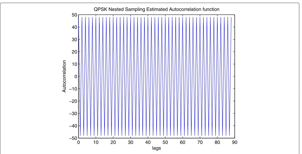
The estimated autocorrelation using nested sampling and coprime sampling structures are plotted in Figures 11 and 12. In the simulation, for nested sampling, we use N1 = 7,N2 = 11, andL = 10. Therefore,Rˆ(k) can be estimated for|k|≤(N1+1)N2−1. For each period, we totally get(N1+1)N2=(7+1)×11=88 samples. While for coprime sampling, we setP=7 andQ=11, for each period, we getPQ=7×11=77 lags ofRˆ(k).

Using the relationship of autocorrelation and the PSD described in Section 3, we could obtain the estimated PSD using nested sampling structure for this QPSK signal as shown in Figure 13. In the simulation, we use 1024 point fast Fourier transform and normalize the PSD. We can see that the estimated PSD is also centered atfc=400 Hz with

symmetric sidelobes on both sides. As stated in Section 3, we can see the PSD is an even function.

0 5 10 15 20 25

0 5 10 15 20 25 30

PSD

N=(N1+1)N2=28

N1=3,N2=7

0 100 200 300 400 500 600 700 800 −60

−50 −40 −30 −20 −10 0

Power Spectral Density of QPSK signal

Frequency, Hz

Normalised PSD, [dB]

Figure 9PSD of the QPSK signal.

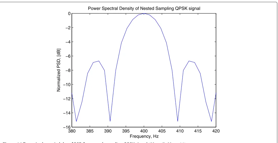
Similarly, if we zoom in this PSD around the central fre-quencyfc, in Figure 14, we could find the main lobe, i.e.,

the bandwidth occupied is approximately 409− 391 ≈ 18 Hz, which is much narrower than that 32 Hz of the PSD of the original QPSK signal. Hence, the spectrum efficiency is improved in the estimation using nested sam-pling structure.

We could also get the estimated PSD using coprime sampling structure for this QPSK signal as shown in Figure 15. In the simulation, we use 1024 point fast Fourier transform and normalize the PSD. We can see that the estimated PSD is also an even function centered at fc=400 Hz with symmetric sidelobes on

both sides.

380 385 390 395 400 405 410 415 420

−50 −45 −40 −35 −30 −25 −20 −15 −10 −5 0

Power Spectral Density of QPSK signal

Frequency, Hz

Normalised PSD, [dB]

0 10 20 30 40 50 60 70 80 90 −50

−40 −30 −20 −10 0 10 20 30 40 50

QPSK Nested Sampling Estimated Autocorrelation function

lags

Autocorrelation

Figure 11Nested sampling estimated autocorrelation of the QPSK signal, whenN1=7,N2=11.

If we zoom in this PSD around the central frequencyfc,

in Figure 16, we could find the main lobe, i.e., the band-width occupied is approximately 411− 389 ≈ 22 Hz, which is near to that estimated using nested sampling and is much narrower than that 32 Hz of the PSD of the original QPSK signal. Hence, the spectrum efficiency is improved in the estimation using coprime sampling structure as well.

Another interesting observation is that the bandwidth of the PSD estimated using coprime sampling is a little larger than that estimated by nested sampling, as shown in our example, the bandwidth for coprime estimated PSD is 411 −389 ≈ 22 Hz, while it is 409− 391 ≈ 18 Hz for nested sampling. This is because for the same num-ber ofPandQ(orN1andN2), the nested sampling could achieveN = (N1+1)N2, while coprime sampling could

0 10 20 30 40 50 60 70 80

−50 −40 −30 −20 −10 0 10 20 30 40 50

QPSK Coprime Estimated Autocorrelation function

lags

Autocorrelation

0 100 200 300 400 500 600 700 800 −35

−30 −25 −20 −15 −10 −5 0

Power Spectral Density of Nested Sampling QPSK signal

Frequency, Hz

Normalized PSD, [dB]

Figure 13PSD of nested sampling QPSK signal(N1=7,N2=11).

only get N = PQ. If N1 = P andN2 = Q, it is obvi-ous that the nested sampling estimate a larger number of Nthan coprime sampling. Refer to the theoretical analy-sis, we could conclude that largerN results in narrower bandwidth, which indicates that ifN1 = PandN2 = Q for nested and coprime sampling, nested sampling would have a more efficient spectrum performance.

By changing different N1 and N2 pairs, as shown in Figure 17, it is obvious that forN1fixed toN1 = 3, with the increase of the value ofN2from 5, 7 to 13, the main lobe of the estimated PSD using nested sampling structure becomes narrower significantly, i.e., the bandwidth occu-pied gets smaller. Here, in the simulation, we normalize the PSD values.

380 385 390 395 400 405 410 415 420

−16 −14 −12 −10 −8 −6 −4 −2 0

Power Spectral Density of Nested Sampling QPSK signal

Frequency, Hz

Normalized PSD, [dB]

0 100 200 300 400 500 600 700 800 −40

−35 −30 −25 −20 −15 −10 −5 0

QPSK Coprime Sampling Estimated Power Sepctrum Density

Frequency, Hz

PSD,[dB]

Figure 15PSD of coprime sampling QPSK signal(P=7,Q=11).

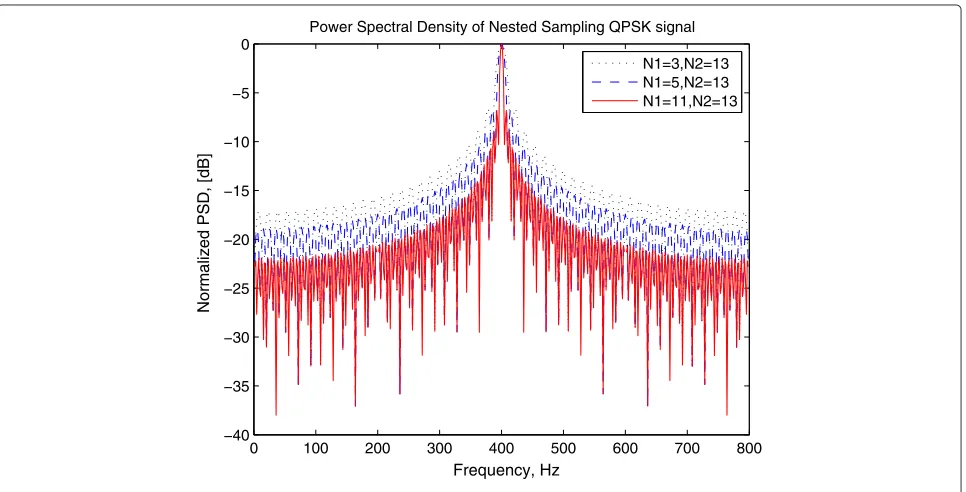
Similarly, Figure 18 shows that with the increase ofN1 fromN1 = 3, 5 toN1 = 11, whileN2fixed toN2 = 13, the main lobe also gets narrower, which also results in the increase of spectrum efficiency.

From the results got from Figures 17 and 18, we con-clude that in the nested sparse sampling process, besides its advantage of less samplers, with N1 and N2 chosen

larger, the bandwidth of the PSD occupied will becomes narrower, which increases the spectrum efficiency.

Similar as nested sampling, as P and Q increase for coprime sampling, the mainlobe of the estimated PSD narrows down as well, which also indicates smaller bandwidth and higher spectrum efficiency as shown in Figure 19, where we increase the second sampler’s

380 385 390 395 400 405 410 415 420

−20 −18 −16 −14 −12 −10 −8 −6 −4 −2 0

QPSK Coprime Sampling Estimated Power Sepctrum Density

Frequency, Hz

PSD,[dB]

0 100 200 300 400 500 600 700 800 −35

−30 −25 −20 −15 −10 −5 0

Power Spectral Density of Nested Sampling QPSK signal

Frequency, Hz

Normalized PSD, [dB]

N1=3,N2=5 N1=3,N2=7 N1=3,N2=13

Figure 17PSD of nested sampling QPSK signal with differentN2.

sampling interval ofQfrom 5, 7, to 13, and in Figure 20, where we increase the first sampler’s sampling interval of Pfrom 3, 5, to 11.

From Figures 17, 18, 19, 20, we could observe nested sparse sampling and coprime sampling could obtain sim-ilar estimated PSD and both are spectrum efficient as the sampling intervals increase, i.e., N1 and N2 for nested sampling, andPandQfor coprime sampling.

7 Conclusions

In this article, the estimated power spectrum density is analyzed and simulated using both nested sampling and coprime sampling structures, which provide us a new way to efficiently use the spectrum.

We give the principle of nested arrays and coprime samplers, and the procedure of how to estimate the autocorrelation and PSD with the sparse samples using

0 100 200 300 400 500 600 700 800

−40 −35 −30 −25 −20 −15 −10 −5 0

Power Spectral Density of Nested Sampling QPSK signal

Frequency, Hz

Normalized PSD, [dB]

N1=3,N2=13 N1=5,N2=13 N1=11,N2=13

0 100 200 300 400 500 600 700 800 −40

−35 −30 −25 −20 −15 −10 −5 0

QPSK Coprime Sampling Estimated Power Sepctrum Density

Frequency, Hz

Normalized PSD,[dB]

P=3,Q=5 P=3,Q=7 P=3,Q=13

Figure 19PSD of coprime sampling QPSK signal with differentQ.

nested and coprime sampling for QPSK signal. We give detailed theoretical analysis of how these two sparse sampling effects the PSD and why it is spectrum effi-ciency with the increase of sampling intervals, i.e., N1 and N2 for nested sampling, P and Q for coprime sampling.

Our simulation results show that with the proper choice of sampling intervals, i.e., making them large enough, the

main lobe of PSD obtained from both nested sampling and coprime sampling is much narrower than the orig-inal QPSK signal. If we choose the sampling intervals larger, the bandwidth occupied will be narrower, which improves the spectrum efficiency. Besides the smaller average rate, the increased spectrum efficiency is a new advantage of both nested sparse sampling and coprime sampling.

0 100 200 300 400 500 600 700 800

−40 −35 −30 −25 −20 −15 −10 −5 0

QPSK Coprime Sampling Estimated Power Sepctrum Density

Frequency, Hz

Normalized PSD,[dB]

P=3,Q=13 P=5,Q=13 P=11,Q=13

Competing interests

The authors declare that they have no competing interests.

Acknowledgements

This study was supported in part by U.S. Office of Naval Research under Grants N00014-13-1-0043, N00014-11-1-0071, N00014-11-1-0865, and U.S. National Science Foundation under Grants CNS-1247848, CNS-1116749, and CNS-0964713.

Author details

1_{Department of Electrical Engineering, University of Texas at Arlington,} Arlington, TX 76019-0016, USA.2_{College of Physics & Electronic Information,} Tianjin Normal University, Tianjin, 300387, China.

Received: 27 January 2013 Accepted: 5 February 2013 Published: 22 February 2013

References

1. TS Rappaport,Wireless Communications: Principles and Practice, 2nd edn. (Prentice Hall PTR, 2001), pp. 278–302

2. TM Cover, JA Thomas,Elements of Information Theory, 2nd edn. (John Wiley & Sons, Inc, Hoboken, New Jersey, 2006)

3. H Mehdi, K Feher, FQPSK, power and spectral efficient family of modulations for wireless communication systems. IEEE Veh. Technol. Conf.3, 1562–1566 (1994)

4. D Li, inAPCC/OECC. A high spectrum efficient multiple access code, (1999), pp. 18–22

5. M-S Alouini, AJ Goldsmith, Area spectral efficiency of cellular mobile radio systems. IEEE Trans. Veh. Technol.48(4), 1047–1066 (1999)

6. JW Burns, inProc. of IEE Conference on Getting the Most Out of Spectrum. Measuring spectrum efficiency-the art of spectrum utilisation metrics, (London, UK, 2002), pp. 1–3

7. P Pal, PP Vaidyanathan, Nested arrays: a novel approach to array processing with enhanced degrees of freedom. IEEE Trans. Signal Process.

58(8), 4167–4181 (2010)

8. P Pal, PP Vaidyanathan, inDigital Signal Processing Workshop and IEEE Signal Processing Education Workshop. Coprime sampling and the MUSIC algorithm, Sedona, 2011), pp. 289–294

9. EJ Candes, MB Wakin, An introduction to compressive sampling. IEEE Signal Process Mag.25(2), 21–30 (2008)

10. P Pal, PP Vaidyanathan, inInternational Conference on Acoustics, Speech and Signal Processing (ICASSP). A novel array structure for

directions-of-arrival estimation with increased degrees of freedom, (Dallas, 2010), pp. 2606–2609

11. PP Vaidyanathan, P Pal, Sparse sensing with co-prime samplers and arrays. IEEE Trans. Signal Process.59(2), 573–586 (2011)

12. DW Ricker,Echo Signal Processing, (Springer, Kluwer Academic Publishers, 2003). pp. 23–26. ISBN 1-4020-7395-X

13. P Stoica, RL Moses,Introduction to Spectral Analysis, 1st edn. (Prentice Hall, Upper Saddle River, New Jersey, 1997), pp. 1–13

doi:10.1186/1687-1499-2013-47

Cite this article as:Chenet al.:Spectrum efficiency of nested sparse

sam-pling and coprime samsam-pling.EURASIP Journal on Wireless Communications

and Networking20132013:47.

Submit your manuscript to a

journal and benefi t from:

7 Convenient online submission

7 Rigorous peer review

7 Immediate publication on acceptance

7 Open access: articles freely available online

7 High visibility within the fi eld

7 Retaining the copyright to your article