R E S E A R C H
Open Access
Robust precoder-decoder design for physical
layer network coding-based MIMO two-way
relaying system
Laddu Keeth Saliya Jayasinghe
*, Nandana Rajatheva and Matti Latva-Aho
Abstract
In this paper, we investigate a robust joint precoder-decoder design scheme for a multiple-input multiple-output physical layer network coding (PNC)-based two-way relay system. An orthogonal training sequence is used to estimate the channels. The estimate is imperfect, and a robust design is proposed to find precoders at the source nodes and decoder at the relay node to facilitate PNC operations during multiple-access stage. Both channel estimation error and antenna correlations are used to formulate the optimization problem to minimize the weighted mean square error (WMSE) under a total power constraint. The problem becomes non-convex, and we propose an algorithm to solve it optimally. During the broadcast stage, an algorithm is proposed to find a precoder at the relay node and decoders at source nodes. The system performance is evaluated with estimation error and antenna correlation parameters. The effect of weighting parameters, relay location, and number of antennas at nodes are also considered in the numerical analysis. Numerical results confirm that our joint precoder-decoder algorithms provide the optimal solution to the minimization of WMSE with the total available power.
Keywords: Bit error rate, Imperfect channel state information, Mean square error, Multiple-input multiple-output, Non-convex optimization, Physical layer network coding
1 Introduction
Cooperative relay communication is introduced to improve the throughput, extend the coverage area, and reduce the energy consumption at the transmitter in wireless communication systems. Relaying information through several hops reduces the need to use large power at the transmitter, which in turn results in a lower level of interference [1]. However, even with these advan-tages, the relay alone has a disadvantage, which is due to half-duplex signaling, i.e., the node cannot transmit and receive signals simultaneously without complicated inter-ference canceling techniques. This reduces the spectral efficiency to a considerable degree.
A significant amount of research effort has been focused on this weakness, and new methods are proposed to over-come the problem. In [2,3], various system models have been studied to provide solutions on this drawback, and
*Correspondence: [email protected]
Centre for Wireless Communications (CWC), Department of Communications Engineering, University of Oulu, Oulu 90570, Finland
more suitable schemes are considered in [4,5] with net-work coding. The authors in [6] proposed a two-way relaying scheme to avoid this problem which requires only two time slots to exchange information between two source nodes as opposed to four in a traditional relay-ing scheme. In these two-way relayrelay-ing systems, the first time slot is known as the multiple access (MA) stage, where both source nodes transmit to the relay at the same time. The second time slot is the broadcasting (BC) stage, where the relay broadcasts the message. Different signal processing methods can be used at the relay node. The most common approach is to employ the amplify-forward (AF) technique at the relay. Recently, new approaches have been investigated using physical layer network cod-ing (PNC) [5,7-9]. The PNC treats interference as useful information. Therefore, PNC improves the capacity of the system and overcomes the shortcomings mentioned ear-lier in the use of relays. In [7,9], the authors performed exclusive-or (XOR) operation at the relay and transmit-ted a modulatransmit-ted signal version of that during the second time slot. Another approach was used in [8], where the
relay estimates the sum of two transmitted messages and forwards it during the next time slot. This is less com-plex and valid for most modulation schemes, and the carrier phase offset between the signals will not affect the performance. Further studies on PNC-based relay-ing are discussed in [5,9,10], and it is found that PNC results in rate improvements of wireless relay systems. Multiple-input multiple-output (MIMO) communication is another spectrally efficient technique that can be used to improve the wireless system performance. MIMO sys-tems have significant performance enhancements over the single-input single-output counterpart [11], and they also provide higher spectral efficiency in the presence of multi-path fading channels [12-14].
Both MIMO and PNC are considered together in some recent research efforts and are identified as potential capacity enhancement techniques for future wireless sys-tems. In most of these studies, it is required to find a relation between two transmitted signals to perform PNC mapping at the relay node. Even though the PNC map-ping is well established for single antenna scenarios, there are no such models to handle MIMO PNC mapping. The authors in [15-18] have used MIMO two-way relaying schemes and discussed the detection mechanisms and performances of such systems. Most of these need com-plex processing at the relay to estimate the XOR of two received signal vectors. A precoder before transmission is proposed in [16], and that reduces the complexity of the receiver at the relay node. The MIMO two-way relaying system can then be shown to produce spatial multiplexing streams; hence, the PNC operation at the relay becomes less complex. In [19], power allocation is considered with zero-forcing precoders at the source nodes to reduce the complexity of PNC operation at the relay node.
Moreover, a joint precoder-decoder design can be thought of as an effective way to reduce the inter-data-stream interference that lowers the complexity of the PNC operation further by placing signal processing capa-bilities at both transmitters and the receiver. Previous studies on AF two-way relaying suggest that the joint precoder and decoder design can achieve more effec-tive capacity enhancements and decoding performances [20-22]. The focus is mainly on minimizing the weighted mean square error (WMSE) in an AF two-way relay sys-tem. In PNC-based two-way relaying systems, the sum-mation of the transmitted signal vectors is needed to map it to either of the XOR version or to transmit the estimated summation. Therefore, MSE is a good mea-sure to design precoders and decoders in PNC-based two-way relaying.
In most of these related cases, channel state informa-tion (CSI) is assumed to be known perfectly in all nodes [19,21-23]. Precoder design at nodes with ideal channel information is not a practical scenario in general. Channel
estimation has errors, and it will affect the system per-formance in a significant manner. Several research studies are carried out by considering various models of imper-fect CSI and their impact on the performance of wireless systems. In [24,25], the authors considered an imperfect CSI model with estimation errors in channel parameters, and they used a training sequence to estimate the chan-nel. In [25-27], transceiver designs for AF MIMO relaying systems are discussed based on this imperfect CSI model. The authors in [28] studied the impact of imperfect CSI in a two-way relaying system. However, their work is lim-ited to a single antenna with expressions for bit error rate (BER) of BPSK scheme. Another imperfect CSI model is discussed in [29-31] for a scenario where the chan-nel parameters are estimated at the receiver and fed to the information to the transmitter and relay node. This can cause feedback delays, and the main concern is the difference between the actual CSI and the outdated CSI. However, the feedback delay of CSI estimates has a sim-ilar model as for the imperfect estimation. In all these models, consideration of imperfect CSI is very impor-tant since focusing only on the perfect information is not sufficient for practical implementations. Having been motivated with these facts, we concentrate our research on robust precoder and decoder designs for MIMO PNC two-way relay system. We also consider the correlation among antennas, which is practical to be assumed in mod-ern compact devices which have sophisticated features. The proposed system design is compared with other alter-natives. Similar studies are not considered in the open literature, to the best of our knowledge.
In this paper, our main focus is to design robust precoders and decoders for source and relay nodes to minimize the WMSE. A channel estimation method is proposed for two-way relaying systems using already-known orthogonal sequence transmission techniques. Errors in the estimation are illustrated, and those are considered in the joint precoder-decoder design prob-lems. Both MA and BC stages are considered in the design of precoders and decoders. Unfortunately, WMSE-based optimization problems become non-convex, and we present methods of solving those by suitable refor-mulation. Different scenarios are investigated to find the impact of the estimation error, antenna correlation, weighting parameters, relay location, and number of antennas to the design. Performance differences are high-lighted, comparing joint precoder-decoder designs with other possibilities.
Notations: Cm×n denotes an m ×n matrix with ele-ments in the complex field. Capital bold letters represent matrices, simple bold letters represent vectors, and sim-ple letters represent scalar variables. Tr(·),(·)−1,(·)T,(·)∗, and(·)H indicate trace, inverse, transpose, conjugate, and hermitian of a matrix, respectively.E{·}and(z)denote the expectation of a random variable and real part ofz. vec(·)gives matrix vectorization operator, and ⊗ repre-sents the Kronecker operator.CN(x,y)denotes a complex Gaussian random variable with meanxand variancey. A similar notation with mean vector and covariance matrix is valid when the variable is a vector.
2 System model and problem formulation
A basic two-way communication system model is consid-ered as shown in Figure 1. The system operates in the time division duplex mode. Source 1 and source 2 are required to exchange data between themselves with the assistance of a relay node. All three nodes haveN anten-nas. The relay is located at a normalized distancedfrom source 1. Source 1-to-relay and source 2-to-relay trans-missions undergo Rayleigh fading withH1 ∈ CN×N and
H2∈CN×N, respectively. Entries ofH1are assumed to be approximatelyd1α CN(0, 1), and entries ofH2are assumed to be approximately (2−1d)α CN(0, 1), whereαis the path loss exponent anddis the normalized distance. The dis-tance between any node to the midpoint of two nodes is considered as the reference distance.
We consider Ri ∈ CN×N as the antenna correlation matrix at sourcei(=1, 2), andRr ∈CN×N is the antenna correlation matrix at the relay node. We consider these matrices to be symmetric. We denoteHm1 = R
1
2 to be the channel matrices from source 1-to-relay and source 2-to-relay. During the BC stage, channel matrices are denoted asHb1 = R
1
During the MA stage, the source nodes transmit their signals and the summation of two signals are received at the relay node. The relay node estimates the sum of the two signals, which is the general scheme of PNC map-ping [8]. However, a problem arises due to channel fading. With fading, the estimation at the relay node becomes exceedingly complex. Therefore, we consider designing precoders at the source nodes and a decoder at the relay node to overcome this problem. Source nodes use pre-codersF1 ∈ CN×N andF2 ∈ CN×N before their trans-missions. The relay node receives both signals at the same time and uses the decoderG∈CN×Nprior to performing any PNC operation as in [8] to estimate the XOR or the summation of two transmitted symbol vectors.
Next, we consider the BC stage of two-way communica-tion. The relay node retransmits the estimated summation during this stage. The source nodes estimate the sum-mation at their nodes and find the respective symbol transmitted by the other node with the help of its own symbol. Here, we consider the precoder at the relay node and decoders at the source nodes. The relay uses the pre-coderFr ∈ CN×N. Both sources 1 and 2 use decoders
G1 ∈ CN×N andG2 ∈ CN×N, and each reconstructs the required symbol with the help of their own information. All nodes dynamically adjust their precoder and decoder matrices with the channel information.
Both stages require CSI knowledge to design the pre-coders and the decoder, and the following procedure is used to estimate channels prior to their data transmission.
2.1 Channel estimation
We assume channel reciprocity and a quasi-static channel environment. The relay transmits an orthogonal sequence to estimate channels at the end of the BC time slot. Both source nodes receive this signal, and they find optimum precoder and decoder matrices. The source nodes then send optimumGandFr to the relay node via dedicated feedback link. We assume that the channel estimation and
y
relay feedback time durations are very small compared to the channel coherence time. Once the two-way relay-ing system is established with optimum precoders and decoders, the source nodes transmit data that are required to exchange between them. Antenna correlations are also assumed to be known.
The relay broadcastsXttraining sequence, whereXtis anN×Nmatrix. The received signal at source 1 is given by the following:
Y1=Hb1Xt+N1, (1)
whereN1is anN×Nmatrix with entries independent and identically distributed (i.i.d.) CN(0,σN2
1). As commonly
used in orthogonal sequence channel estimation [24], we useXt= R− mit powerPt. Source 1 pre-multiplies the received signal matrix byR−
1 2
1 and post-multiplies it byX−1. Therefore, the received channel matrixHT1 is given by the following:
criterion is used to obtain the channel estimate fromHT1. The MMSE estimate is presented as follows:
¯
The estimation error can be obtained [27] as
R− matrix now consists of MMSE estimation and the estimation error part as
HT1 = ¯HT1 +R−
A similar result is valid for the estimation ofHT2, and it is given byHT2 = ¯HT2 +R−12
Since we assume the channel reciprocity, using (3) and (4), we can write the source-to-relay channels Hmi as follows:
Correlation matrices are symmetric, and for sim-plicity, we denote H¯mi = R
, where these represent each channel matrix with a mean part and an estimation error part. We use these estimated channels to design precoders and decoder.
2.2 Physical layer network coding
During data transmission, modulated symbol vec-tors are fed into sources 1 and 2, with each given as x1 = (x11, x12, x13,. . .,x1N)T and
x2 = (x21, x22, x23,. . .,x2N)T, where xii ∈ C and
Ex{xixHi } = IN (i = 1, 2). The relay node estimates the summation of modulated signals (x1+x2) and transmits it during the next time slot. This is more general and a valid PNC scheme for any modulation alphabet. For simple modulation schemes like QPSK, this summation of two signals can be mapped to XOR of two transmit-ted unmodulatransmit-ted information [8]. During the next time slot, the modulated symbol of XOR version will then be transmitted. In summary, we can carry out PNC for any case if we design the precoders and decoders to mini-mize the MSE between received signal and summation of modulated signals.
During the first time slot, the received signal vectory∈
CN×1at the relay is given by the following:
y=GHm1F1x1+GHm2F2x2+Gn, (6)
where n ∼ CN(0,σ2IN). The relay node estimates the
x1+x2, and this leads us to considerNnumber of sep-arate spatial streams. Therefore, the received signal atith streamyi can be used to obtain an estimate correspond-ing tox1i+x2i. This scheme reduces the complexity of the PNC mapping at the relay [32]. We denote the estimation ofx1i+x2iasx3i, andx3ibroadcasts to other nodes during the next time slot.
During the second time slot, the received signal vector
y1∈CN×1at the source 1 is given as follows:
y1=G1Hb1Frx3+G1n1, (7)
where x3 = (x31, x32, x33,. . .,x3N)T and n1 ∼
CN(0,σ2IN). Similarly, received signal vectory2∈CN×1 at the source 2 is given as follows:
y2=G2Hb1Frx3+G2n1, (8)
a similar manner as for the case where there are equal number of antennas at the nodes.
Accuracy of the PNC mapping is dependent on the esti-mated summation of two symbols. Therefore, it is evident that the optimum joint design is required to have accurate estimation process. Problem formulation and the solving method for designing optimum precoders and decoders are described in the next sections of the paper.
2.3 Problem formulation
As two-way communications have two phases, we can consider the analysis separately for both phases. For each phase, the total power can be limited, which can occur in many practical scenarios. Therefore, we considerPTas the maximum total transmitted power available in each time slot. A similar problem formulation and solving procedure is valid for individual power constraints of nodes.
2.3.1 Multiple-access stage
In this stage, both source nodes transmit to relay, and the transmitted powers of source nodes should satisfy the following constraint:
Tr(F1FH1)+Tr(F2FH2)≤PT, (9) The received signal (6) during the MA stage is used to estimatex1+x2. The estimation error vectoremcan be defined as follows:
em=GHm1F1x1+GHm2F2x2+Gn−x1−x2 (10) Data streams may need different quality of service (QoS). We facilitate this by introducing weights for differ-ent streams. A diagonalN × N positive definite weight matrixWis used for that purpose. We express WMSE at the MA stage as follows:
WMSEm=Ex,n{W1/2em2}
We need to minimize WMSEm during the MA stage subject to the total power constraint to find optimum precoders and decoders. However, for given channel instances ofHm1andHm2, the estimation error becomes
a random variable. We have to consider this channel esti-mation error with WMSEm. The error has a Gaussian dis-tribution, and we focus on the expected value of WMSEm, given as follows:
EE{WMSEm} =EE{Tr(W(GHm1F1−IN)
×(GHm1F1−IN)H+W(GHm2F2−IN) ×(GHm2F2−IN)H+σ2WGGH)}. (13) Channel estimates in (5) consist of the MMSE value and the error part asHmi= ¯Hmi+Emifori=1, 2. Therefore, expanding (13) into the following:
EE{WMSEm} =
Moreover, we can expand the following term with the expectation as follows:
between trace and vectors to simplify (16) into the following:
EE{Tr(PiEiTQiE∗i)} =EE{vec(E∗i)vec(PiETiQi)} =EE{vec(E∗i)(Qi⊗Pi)vec(ETi )} =Tr((Qi⊗Pi)E{vec(ETi)vec(E∗i)}).
(17) We know thatE{vec(ETi)vec(E∗i)} = σi2Iand using the relation Tr((Qi⊗Pi)) = Tr(Qi)Tr(Pi), we can find the following expression for (15):
EE{WMSEm} = 2
i=1
Tr(WGH¯miFiFHi H¯HmiGH−WGH¯miFi
−WFHi H¯HmiGH+W)
+ 2
i=1
σi2Tr(Qi)Tr(Pi)+Tr(σ2WGGH)
(18) Next, we formulate the optimization problem to min-imize expected value of WMSEm under a limited avail-able transmit power at source nodes as presented in Problem 1:
Problem 1.
min F1,F2,G
EE{WMSEm}
subject to Tr(F1FH1)+Tr(F2FH2)≤PT
(19)
This is a non-convex optimization problem. In Section 3, we propose an algorithm to solve this optimally.
2.3.2 Broadcasting stage
Estimatedx1+x2, i.e.,x3broadcasts during this time slot. Relay uses Fr precoder and transmitsx3to both source nodes. Sources 1 and 2 now haveG1 and G2 decoders, respectively. At sourcei(= 1, 2), it estimatesx3and uses that to find desired symbol.
Similar to the MA stage, the joint design is considered to minimize the WMSE of received signals. We considered all nodes to satisfy a total power constraint for their trans-mission. Therefore, during the BC stage, transmit power at the relay node should satisfy the following constraint:
Tr(FrFHr)≤PT/2. (20)
This constraint becomesPT/2 becauseEx{x3xH3}is now equal to 2IN; ebi is the estimation error vector at ith source. It is given as follows:
ebi=GiHbiFrx3+Gini−x3. (21)
We use the similar weights for different streams as in multiple-access analysis. WMSE at sourceiis denoted as WMSEiand is given by the following:
WMSEi=2W(GiHbiFr−IN)(GiHbiFr−IN)H +σ2WGiGHi i=1, 2. (22)
Hbi has an error component. Therefore, the expected value of WMSEiis considered in the optimum precoder-decoder design. A similar procedure as in the MA stage is valid to find the expected value of WMSEi. We find WMSEias follows:
EE{WMSEi} =2Tr(WGiH¯miT FrFHr H¯∗miGHi
−WGiH¯TmiFr−WFHrH¯∗miGHi +W) +2σi2Tr(Li)Tr(K)
+Tr(σ2WGiGHi ) i=1, 2, (23)
whereLi=
IN+σi2R−i 1 −1
2
GHi WGHi
IN+σi2R−i1 −1
2
andK=R12 rFrFHr R
1 2 r.
Both source nodes are trying to minimize expected val-ues of the WMSE1and WMSE2during the BC stage. We are not considering a greedy approach, i.e., every node is trying to minimize its own WMSE component. Equal proportions of WMSE are considered to find optimum precoder and decoders. Therefore, we consider the sum of two components, and the problem is formulated in Problem 2.
Problem 2.
min Fr,G1,G2
1
2EE{WMSE1} + 1
2EE{WMSE2} subject to Tr(FrFHr )≤PT/2.
(24)
This problem is a non-convex problem, and we propose solutions in the next section.
3 Optimum joint designs
Here, we propose optimum algorithms to solve the non-convex optimization Problems 1 and 2. We can prove that both problems have global minimums (Appendix), and we can achieve those in our proposed algorithms.
3.1 Optimum precoder-decoder design for MA stage Here, we propose an algorithm to solve Problem 1 by dividing it into two sub-problems. Mainly, we can find two different sets of variables in this problem. Precoders can be categorized into one set of variables and the decoder into the other. With these observations, we proceed with the following method.
These are identified as the two sub-problems of the origi-nal problem. The solutions of these two sub-problems are used in the next iteration. The problem is solved iteratively untilG,F1, andF2converge to become fixed matrices.
3.1.1 Sub-problem 1A
We considerF1andF2as fixed. Therefore, the problem is reduced to the following form:
min
G EE{WMSEm}. (25)
The power constraint is independent ofG. Therefore, we take derivative of the objective function and make that equal to zero. The solution forGis the optimum one dur-ing that iteration and is given as a function ofF1,F2, and
We considered complex-valued matrix function differ-entiation as in [33] to obtain the results.
3.1.2 Sub-problem 1B
We consider a similar problem as in (19) and keep G
as fixed. Therefore, we have two variables, F1 and F2. Optimization problem can be reformulated as follows:
min
A variable transformation is considered before solving this problem. We define new matrix variablesF∈C2N×2N
asF = (F1 0N×N ; 0N×N F2). We also define the fol-lowing matricesAandCto simplify the other parameters, whereA=(W12GH¯m1 0N×N ; 0N×N W12GH¯m2)and
The reformulated optimization problem is then given as follows: whereAHAis a positive semi-definite matrix. This is con-vex and is known as the quadrature matrix programming problem. We transpose this into a quadratically con-strained quadratic programming (QCQP) problem which is given by the following:
min can be easily solved with QCQP solvers, which ultimately give optimum matrices ofF1andF2in that iteration. In the numerical analysis, we used interior point method to solve this sub-problem.
We solve Problem 1 using the two sub-problems men-tioned. First, we start by fixing F1 andF2, giving initial values. Next, we solve sub-problem 1A to find the opti-mumG. We then useGto solve sub-problem 1B, which gives F1 andF2. TheseF1 andF2 will be used again to solve the sub-problem 1A, which updates the optimum
G. We solve iteratively until the problem gives convergent solutions. The final algorithm is given as follows:
The proposed algorithm converges rapidly with a small number of iterations. Initialization point does not have any effect on the final convergence point. We find that this always reaches the global optimum.
3.2 Optimum precoder-decoder design for BC stage During the BC stage, the requirement is that source nodes should find decoders and the relay node should find the precoder. Those can be found by solving Problem 2. Simi-lar to the previous stage, we can use an iterative algorithm to find the optimum design. First, we consider the fixedFr matrix, and findG1andG2. Next, we fixG1andG2and find Fr. These can be identified as two sub-problems of the original Problem 2.
3.2.1 Sub-problem 2A
Algorithm 1Algorithm for solving Problem 1
1: Initialize
i. Initialize precoder matrices.F1=
initial point). Solve sub-problem 1A to find
optimumG.
ii. FixGobtained from (2.i). Solve sub-problem 1B to find optimumF. Then obtainF1andF2.
3: Until
i. WMSEmreduces during each step. Continue
till it converges, i.e.,
|WMSEkm+1−WMSEkm| ≤, wherek denotes the iteration number and (<<1)is a positive constant.
The power constraint is independent of G1 and G2. Therefore, we can derive the objective function withG1 andG2and make those equal to zero. Solutions are given as follows:
In here, we considerG1 andG2 as fixed. Therefore, we have one variable Fr. The second sub-problem can be found as follows:
We can transform this problem into QCQP, which is given by the following:
min and can be solved with any QCQP solver. We used inte-rior point method to solve this in our numerical analy-sis. Finally, Problem 2 can be solved with the following algorithm.
Algorithm 2Algorithm for solving Problem 2
1: Initialize
i. Initialize precoder matrices.Fr =
PT 4NIN.
2: Repeat
i. FixFrobtained from (2.ii.) (Or (1.i) at initial
point). Solve sub-problem 2A to find optimum G1, andG2.
ii. FixG1, andG2obtained from (2.i). Solve
sub-problem 2B to find optimumFr.
3: Until
(a) WMSE1+WMSE2reduces in each step.
Continue till it converges, i.e.,
|WMSEk1+1+WMSE2k+1−WMSEk1−WMSEk2| ≤
, wherek denotes the iteration number, and
(<<1)is a positive constant.
The proposed algorithm converges with a small num-ber of iterations, and initial point does not have any effect on the final solution. As we explain in the Appendix, this reaches global optimum.
We use these two algorithms to find precoders and decoders in both MA and BC stages. These precoder and decoder matrices are dependent on the instanta-neous channel information, and nodes dynamically adjust according to the CSI.
4 Numerical results
parameters on error probability. Rayleigh fading channels are considered, and relay location is normalized from the source 1-to-relay distance. Numerical simulations are also assume that the transmitted symbols be uniformly dis-tributed with unit magnitude. During the MA stage, the relay receiver estimates the summation of symbols. Dur-ing the BC stage, source nodes estimate the broadcast symbol by the relay node (estimated sum of two symbols). We have considered WMSE minimization problems at both MA and BC stages. Therefore, we focus on the error analysis after a complete cycle. Antenna correlation of source 1 is defined by(R1)ij=ρS1|i−j|, whereρS1is the cor-relation coefficient. A similar definition is used forR2and
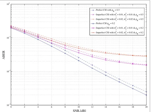
Rrwith correlation coefficientsρS2andρR, respectively. Figure 2 shows the average BER (ABER) performance with the transmit signal-to-noise ratio (SNR) (γ) of a modulated symbol. Performance metric ABER considers average error rates at both source nodes after a complete cycle. The weighting matrix is considered asW = N1IN,
the relay is located at midpoint (d = 1), the number of antennas isN=2, convergence constant=0.0001, and the total transmit powerPTis selected such thatPT/σ2= 8γ. We consider both perfect and imperfect channel esti-mation scenarios with different relay correlation coeffi-cientsρR. Here, the estimation error partEmiof channel estimation is considered as in (5), and the error variance σi2is used to quantify the contribution of the error. The error varianceσi2is obtained withσi2=σN2
iTr(R
−1 r )/Pt. In the simulations, we changePt/σN2ito vary theσi2. As seen in the Figure 2, the joint precoder-decoder design with the perfect channel knowledge performs better than the rest. When the estimation error increases, the performance reduces. This figure also shows the relay antenna corre-lation effect on the average BER. The joint design for the perfect channels is highly sensitive to antenna correlation of the relay. When the estimation error becomes higher, the antenna correlation has less effect, which can be seen from the case having σi2 = 0.02. Pt/σN2i is considered
0 2 4 6 8 10 12 14 16 18 20
10−3 10−2 10−1 100
SNR,[dB]
ABER
Perfect CSI with ρR = 0.5 Imperfect CSI with σ12 = 0.01, σ
2
2 = 0.01 & ρ R = 0.5
Imperfect CSI with σ
1 2
= 0.02, σ
2 2
= 0.02 & ρ
R = 0.5
Perfect CSI ρR = 0.2
Imperfect CSI with σ12 = 0.01, σ 2
2 = 0.01 & ρ R = 0.2
Imperfect CSI with σ
1 2
= 0.02, σ
2 2
= 0.02 & ρ
R = 0.2
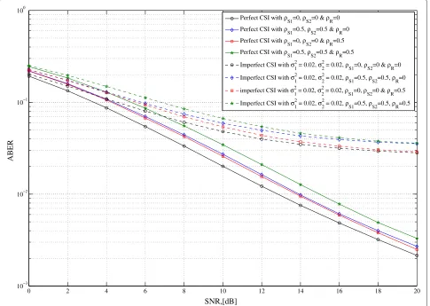
as 21.2 and 20.2 dB for cases ρR = 0.5 and ρR = 0.2, respectively. Here, the difference in the error performance is very small. Similarly, Figure 3 presents the case when all nodes have antenna correlation. It is clear that when all nodes have some amount of correlation, the performances become degraded. A significant variance is visible with a small channel estimation error (or perfect estimation).
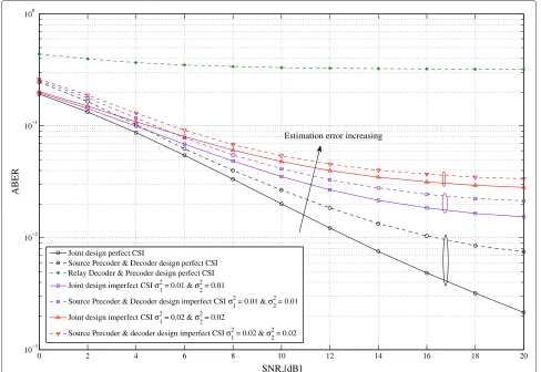
Next, we consider two other design schemes to compare the benefits of the proposed scheme. The first scheme considers signal processing at the source nodes during both MA and BC stages. During the MA stage, the opti-mum precoder design is considered to minimize WMSE at the source nodes. Here, the decoder is not taken into account. Similarly, at the BC stage, the decoder design is considered to minimize WMSE, where the precoder at the relay is not considered. The second scheme is the opposite of the first scheme. During the MA stage, the decoder design is considered at the relay node. During the BC stage, only the precoder design is considered. These two schemes are useful to find how beneficial the joint design is compared to other possible designs. Figure 4
shows the ABER variation of these three schemes with the transmit SNR. We considerW = N1IN,N = 2, = 0.0001,PT/σ2 = 8γ, andd = 1. It shows that the joint design scheme performs better than the rest. In the low SNR region, the first design scheme gives a small varia-tion in ABER performance, whereas when SNR increases, the joint design has a significant performance improve-ment. This difference is reduced when the error variance becomes high.
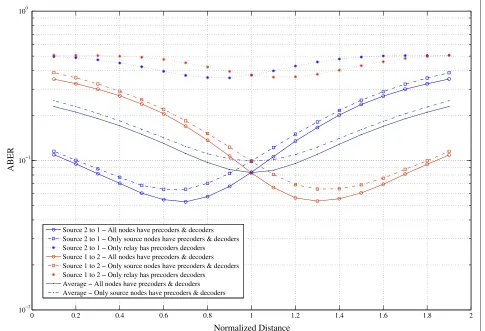
In Figure 5, we considered the ABER variation with normalized distanced. We consider error rates of bidirec-tional transmissions and also their corresponding average. We considerN =2, =0.0001,γ =4 dB, andPT/σ2= 32 dB. It can be seen that the joint design performs bet-ter than the rest for all relay locations. However, when the relay is near one source, the precoder design also gives better results.
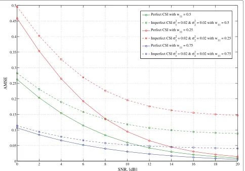
We consider different weight parameters to observe their effect on MSE. Figure 6 shows the average MSE (AMSE) of the received signal at the first antenna of the relay (during MA stage) with the transmit
0 2 4 6 8 10 12 14 16 18 20
10−3 10−2 10−1 100
SNR,[dB]
ABER
Perfect CSI with ρS1=0, ρS2=0 & ρR=0 Perfect CSI with ρ
S1=0.5, ρS2=0.5 & ρR=0
Perfect CSI with ρ
S1=0, ρS2=0 & ρR=0.5
Perfect CSI with ρS1=0.5, ρS2=0.5 & ρR=0.5 Imperfect CSI with σ
1 2
= 0.02, σ
2 2
= 0.02, ρ
S1=0, ρS2=0 & ρR=0
Imperfect CSI with σ
1 2
= 0.02, σ
2 2
= 0.02, ρ
S1=0.5, ρS2=0.5, ρR=0
imperfect CSI with σ12
= 0.02, σ22
= 0.02, ρS1=0, ρS2=0 & ρR=0.5 Imperfect CSI with σ
1 2
= 0.02, σ
2 2
= 0.02, ρ
S1=0.5, ρS2=0.5, ρR=0.5
0 2 4 6 8 10 12 14 16 18 20 10−3
10−2 10−1 100
SNR,[dB]
ABER
Joint design perfect CSI
Source Precoder & Decoder design perfect CSI Relay Decoder & Precoder design perfect CSI Joint design imperfect CSI σ
1 2
= 0.01 & σ
2 2
= 0.01 Source Precoder & Decoder design imperfect CSI σ
1 2
= 0.01 & σ
2 2
= 0.01 Joint design imperfect CSI σ12
= 0.02 & σ22
= 0.02 Source Precoder & decoder design imperfect CSI σ
1 2
= 0.02 & σ
2 2
= 0.02
Estimation error increasing
Figure 4ABER versus transmit SNR: three different design schemes.Average BER variation with SNR (γ) for three different design schemes. N=2,PT/σ2=8γ.
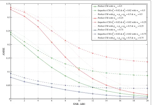
SNR. We consider each node to have two anten-nas N = 2, = 0.0001, and the total trans-mit power PT/σ2 = 8γ. Antenna correlation is not considered; it focuses only on the channel esti-mation errors. Two data streams are considered with three possible weight values (0.25, 0.50, 0.75) for stream 1. AMSE reduces with the transmit SNR for every weight scenario. Also, when the weight parameter is higher, it further reduces the AMSE. This is therefore suitable to provide specific QoS requirements for mul-tiple streams. Figure 7 shows a similar numerical anal-ysis for the BC stage. The received signal at source 2 is used to find AMSE. In addition to the previ-ous case, we assume the antenna correlation at the nodes, and it can be seen that the correlation has less impact on the performance compared to channel estimation errors.
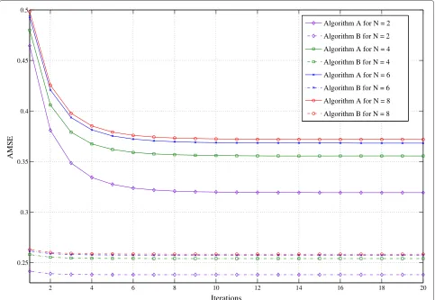
Figure 8 shows the average number of iterations required for Algorithms 1 and 2 to converge with the number of antennas. We use W = N1IN, γ = 4 dB, σ1 =σ2 = 0.02,ρS1= ρS2 = ρR = 0.5, = 0.0001 and
PT/σ2 = 4Nγ. When the system has a higher number of antennas, more iterations are needed for Algorithm 1. These are realistic numbers, which can be used in practice with large MIMO systems. Algorithm 2 converges with a fewer number of iterations, and the variation with the initial point is extremely low.
5 Conclusions
0 0.2 0.4 0.6 0.8 1 1.2 1.4 1.6 1.8 2 10−2
10−1 100
Normalized Distance
ABER
Source 2 to 1 − All nodes have precoders & decoders Source 2 to 1 − Only source nodes have precoders & decoders Source 2 to 1 − Only relay has precoders decoders
Source 1 to 2 − All nodes have precoders & decoders Source 1 to 2 − Only source nodes have precoders & decoders Source 1 to 2 − Only relay has precoders decoders
Average − All nodes have precoders & decoders Average − Only source nodes have precoders & decoders
Figure 5ABER versus normalized distance (d).Average BER variation with normalized distance (d) for three different design schemes.N=2,
γ=4 dB, andPT/σ2=32 dB.
the joint precoder-decoder design performs better than the other schemes. The weight matrix can be used to provide QoS requirements of multiple data streams in MIMO two-way channels. The midpoint is seen to be the best location for the relay node to assist two-way communication. The proposed algorithm converges in a fewer iterations, and the number of iterations increases slowly with the number of antennas. These findings can help to have less complex PNC operation, improve the error performances, and mitigate the half-duplex issue of cooperative relays.
Appendix
Existence of a global solution Problem 1
As in ([34], p. 133, Sec. 4.1.3), an optimization prob-lem with several variables can always be minimized by initially minimizing some of the variables and then minimizing the remaining ones. Therefore, the opti-mization problem given in (19) can be reformulated as follows:
min F1,F2,Tr(F1FH
1)+Tr(F2FH2)≤PT min G[F1,F2] ×EE{WMSEm
F1,F2,G[F1,F2]
},
(36)
where G = G[F1,F2] is a function ofF1 andF2. Inner optimization in problem (36) has no constraints, and the solution forG[F1,F2] is given as follows:
G[F1,F2]=(FH1H¯Hm1+FH2H¯Hm2) (37) ×(H¯m1F1FH1H¯m1H + ¯Hm2F2FH2H¯Hm2 +Tr(σ12Q1+σ22Q2)Rr+σ2IN)−1.
Then, we can replaceGwith that, and the final objective function becomes variables ofF1andF2:
min F1,F2,Tr(F1FH
1)+Tr(F2FH2)≤PT
0 2 4 6 8 10 12 14 16 18 20 0
0.05 0.1 0.15 0.2 0.25 0.3 0.35 0.4 0.45 0.5
SNR, [dB]
AMSE
Perfect CSI with w
11 = 0.5
Imperfect CSI σ12 = 0.02 & σ 2 2
= 0.02 with w
11 = 0.5
Perfect CSI with w
11 = 0.25
Imperfect CSI σ12 = 0.02 & σ 2 2
= 0.02 with w
11 = 0.25
Perfect CSI with w
11 = 0.75
Imperfect CSI σ12 = 0.02 & σ 2 2
= 0.02 with w
11 = 0.75
Figure 6AMSE versus transmit SNR: weight parameters in MA stage.Average MSE variation with SNR (γ) for different weight parameters in multiple access stage.N=2,PT/σ2=8γ.
where
EE{WMSEm[F1,F2]}
= 2
i=1 Tr
WG[F1,F2]H¯miFiFHi H¯HmiG[F1,F2]H
−WG[F1,F2]H¯miFi −WFHi H¯HmiG[F1,F2]H+W
+Tr(σ2WGGH)
+ 2
i=1
σi2Tr(IN+σi2R−i 1)−1FiFHi
×TrRrG[F1,F2]HWG[F1,F2]. (39)
We can see that the feasible set of the optimization prob-lem (38) is closed and bounded as in ([34], p. 30, Sec. 2.2.3). Since this is closed and bounded, the feasible set is compact according to ([35], p. 653, A.6 (g)). Addition-ally, the objective function (39) is continuous at all points of the feasible set. Therefore, according to the theorem in
([35], p. 654, A.8), there exists a global minimum for the problem (38). Finally, we can conclude that in ([34], p. 130, Sec. 4.1.3), there exists a global minimum for the original problem.
Problem 2
A similar procedure is valid to show the existence of a global minimum for Problem 2. However, for the sake of completeness, we describe it as given in this section. Opti-mization problem in (24) can be reformulated as follows ([34], p. 133, Sec. 4.1.3):
min Fr,Tr(FrFHr)≤PT/2
min G1[Fr],G2[Fr]
× 1
2EE{WMSE1[Fr,G1[Fr] ]}
+ 1
2EE{WMSE2[Fr,G2[Fr] ]} (40)
0 2 4 6 8 10 12 14 16 18 20 0
0.05 0.1 0.15 0.2 0.25 0.3 0.35
SNR, [dB]
AMSE
Perfect CSI with w
11 = 0.5
Imperfect CSI σ
1 2
= 0.02 & σ
2 2
= 0.02 with w
11 = 0.5
Perfect CSI with ρs1 = ρs2= ρR = 0.5 & w
11 = 0.5
Perfect CSI with w
11 = 0.25
Imperfect CSI σ12 = 0.02 & σ 2
2 = 0.02 with w 11 = 0.25
Perfect CSI with ρ
s1 = ρs2= ρR = 0.5 & w11 = 0.25
Perfect CSI with w
11 = 0.75
Imperfect CSI σ
1 2
= 0.02 & σ
2 2
= 0.02 with w
11 = 0.75
Perfect CSI with ρs1 = ρs2= ρR = 0.5 & w
11 = 0.75
Figure 7AMSE versus transmit SNR: weight parameters in BC stage.Average MSE variation for source 1 with SNR (γ) for different weight parameters in broadcasting stage.N=2,PT/σ2=8γ.
which are independent with Fr which is fixed. Also, the problem has no constraints. Therefore, the problem can be solved by taking derivatives and making those equal to zero.
Gi[Fr]=
2FHrH¯∗mi
×2H¯TmiFrFHr H¯∗mi+2σi2Tr(K)
×IN+σi2R−i 1 −1+
σ2IN −1
i=1, 2. (41)
Next, we can replace G1[Fr] and G2[Fr] with above-mentioned solutions to find the following optimization problem:
min Fr,Tr(FrFHr)≤PT/2
1
2EE{WMSE1[Fr]} + 1
2EE{WMSE2[Fr]} (42)
where
EE{WMSEi[Fr]}
=2TrWGi[Fr]H¯TmiFrFHrH¯∗miGi[Fr]H
−WGi[Fr]H¯TmiFr−WFHrH¯∗miGi[Fr]H+W
+2σi2Tr(IN+σi2Ri−1)−1Gi[Fr]HWGi[Fr]H
×TrRrFrFHr
+Trσ2WGi[Fr]Gi[Fr]H i=1, 2. (43)
2 4 6 8 10 12 14 16 18 20 0.25
0.3 0.35 0.4 0.45 0.5
Iterations
AMSE
Algorithm A for N = 2
Algorithm B for N = 2
Algorithm A for N = 4
Algorithm B for N = 4
Algorithm A for N = 6
Algorithm B for N = 6
Algorithm A for N = 8
Algorithm B for N = 8
Figure 8AMSE versus number of iteration.Average number of iteration to converge with the number of antennas.γ=4 dB andPT/σ2=4Nγ.
Competing interests
The authors declare that they have no competing interests.
Acknowledgements
The authors would like to acknowledge the support of the European Commission by partially funding this work, under project
FP7-ICT-2009-4-247733-EARTH, Finnish Funding Agency for Technology and Innovation (Tekes), Renesas Mobile, Nokia Siemens Networks, Elektrobit.
Received: 1 January 2013 Accepted: 16 May 2013 Published: 26 May 2013
References
1. JN Laneman, GW Wornell, Energy-efficient antenna sharing and relaying for wireless networks. Proc. IEEE, Wireless Commun. Networ. Confe.1, 7–12 (2000)
2. G Scutari, S Barbarossa, D Ludovici, inProceedings of 4th IEEE Workshop on Signal Processing Advances in Wireless Communications SPAWC 2003 Rome. Cooperation diversity in multihop wireless networks using opportunistic driven multiple access (IEEE Piscataway, 2003), pp. 170–174
3. Munoz O, A Agustin, J Vidal, inInternational Zurich Seminar on
Communications (IZS), Zurich. Cellular capacity gains of cooperative MIMO transmission in the downlink (Piscataway, 2004), pp. 22–26
4. S Katti, H Rahul, W Hu, D Katabi, M Médard, J Crowcroft, XORs in the air: practical wireless network coding. IEEE/ACM Trans. Netw. (TON).16(3), 497–510 (2008)
5. P Larsson, N Johansson, K Sunell, Coded bi-directional relaying. Proc. IEEE 63rd Veh. Technol. Conf.2, 851–855 (2006)
6. B Rankov, A Wittneben, Spectral efficient protocols for half-duplex fading relay channels. IEEE J. Sel. Areas Commun.25(2), 379–389 (2007) 7. S Zhang, SC Liew, PP Lam, inProceedings of the 12th Annual International
Conference on Mobile Computing and Networking (MobiCom ’06). Hot topic: physical-layer network coding (ACM New York, 2006), p. 365
8. S Zhang, SC Liew, L Lu, inProceedings of IEEE Global Telecommunications Conference (GLOBECOM), Los Angeles. Physical layer network coding schemes over finite and infinite fields (IEEE Piscataway, 2008), pp. 1–6 9. P Popovski, H Yomo, Bi-directional amplification of throughput in a
wireless multi-hop network. Proc. IEEE, 63rd Vehi. Tech. Conf.2, 588–593 (2006). VTC 2006-Spring
10. B Nazer, M Gastpar, Compute-and-forward: Harnessing interference through structured codes. IEEE Trans. Infor. Theo.57(10), 6463–6486 (2011)
11. IE Telatar, Capacity of multi-antenna Gaussian channels. Euro. Trans. Telecommun.10(6), 585–596 (1999)
12. JH Winters, J Salz, RD Gitlin, The impact of antenna diversity on the capacity of wireless communication systems. IEEE Trans. Commun.42(2), 1740–1751 (1994)
13. MO Hasna, MS Alouini, End-to-end performance of transmission systems with relays over Rayleigh-fading channels. IEEE Trans. Wireless Commun. 2(6), 1126–1131 (2004)
14. GK Karagiannidis, TA Tsiftsis, RK Mallik, Bounds for multihop relayed communications in Nakagami-m fading. IEEE Trans. Commun.54, 18–22 (2006)
15. S Xu, Y Hua, inProceedings of IEEE International Conference on Acoustics Speech and Signal Processing (ICASSP), Texas. Source-relay optimization for a two-way MIMO relay system (IEEE Piscataway, 2010), pp. 3038–3041 16. S Kim, J Chun, inProceedings of IEEE Wireless Communications and
MIMO pre-equalizer using modulo in two-way channel (IEEE Piscataway, 2008), pp. 517–521
17. H Yang, K Lee, J Chun, inProceedings of IEEE International Conference on Communications (ICC) 2007 Glasgow. Zero-forcing based two-phase relaying (IEEE Piscataway, 2007), pp. 5224–5228
18. S Zhang, S Liew, inProceedings of IEEE Wireless Communications and Networking Conference (WCNC), Sydney. Physical layer network coding with multiple antennas (IEEE Piscataway, 2010), pp. 1–6
19. LKS Jayasinghe, N Rajatheva, M Latva-aho, inProceedings of IEEE Wireless Communications and Networking Conference (WCNC), Paris. Energy efficient MIMO two-way relay system with physical layer network coding (IEEE Piscataway, 2012), pp. 1–5
20. W Guan, H Luo, Joint MMSE transceiver design in non-regenerative MIMO relay systems. IEEE Commun. Lett.12(7), 517–519 (2008)
21. KJ Lee, KW Lee, H Sung, I Lee, inProceedings of IEEE 69th VTC Spring 2009 Barcelona. Sum-rate maximization for two-way MIMO
amplify-and-forward relaying systems (IEEE Piscataway, 2009), pp. 1–5 22. S Xu, Y Hua, Optimal design of spatial source-and-relay matrices for a
non-regenerative two-way MIMO relay system. IEEE Trans. Wireless Commun.10(5), 1645–1655 (2011)
23. R Wang, M Tao, Joint source and relay precoding designs for MIMO two-way relaying based on MSE criterion. Tran. Sign. Proc.60(3), 1352–1365 (2012)
24. B Hassibi, B Hochwald, How much training is needed in multiple-antenna wireless links?. IEEE Trans. Infor. Theo.49(4), 951–963 (2003)
25. C Xing, S Ma, Y Wu, Robust joint design of linear relay precoder and destination equalizer for dual-hop amplify-and-forward MIMO relay systems. IEEE Trans. Sig. Proc.58(4), 2273–2283 (2010)
26. C Xing, Z Fei, Y Wu, S Ma, J Kuang, inProceedings of IEEE ICSPCC 2011 Shaanxi. Robust transceiver design for AF MIMO relay systems with column correlations (IEEE Piscataway, 2011), pp. 1–6
27. M Ding, S Blostein, MIMO minimum total MSE transceiver design with imperfect CSI at both ends. IEEE Trans. Sig. Proc.57(3), 1141–1150 (2009) 28. Z Ding, KK Leung, Impact of imperfect channel state information on
bi-directional communications with relay selection. IEEE Trans. Sig. Proc. 59(11), 5657–5662 (2011)
29. S Thoen, L Van der Perre, B Gyselinckx, M Engels, Performance analysis of combined transmit-SC/receive-MRC. IEEE Trans. Commun.49, 5–8 (2001) 30. HA Suraweera, TA Tsiftsis, GK Karagiannidis, M Faulkner, inProceedings of
IEEE GLOBECOM 2009 Hawaii. Effect of feedback delay on downlink amplify-and-forward relaying with beamforming (IEEE Piscataway, 2009), pp. 1–6
31. G Amarasuriya, C Tellambura, M Ardakani, inProceedings of IEEE GLOBECOM 2010 Miami. Feedback delay effect on dual-hop MIMO AF relaying with antenna selection (IEEE Piscataway, 2010), pp. 1–5 32. T Koike-Akino, P Popovski, V Tarokh, Optimized constellations for two-way
wireless relaying with physical network coding. IEEE J. Sel. Areas Commun.27(5), 773–787 (2009)
33. A Hjorungnes, D Gesbert, Complex-valued matrix differentiation: techniques and key results. IEEE Trans. Sign. Proces.55(6), 2740–2746 (2007)
34. S Boyd, L Vandenberghe,Convex Optimization. (Cambridge University Press, Cambridge, 2004)
35. DP Bertsekas,Nonlinear Programming. (Athena Scientific, Nashua, 1999)
doi:10.1186/1687-1499-2013-137
Cite this article as:Saliya Jayasingheet al.:Robust precoder-decoder design
for physical layer network coding-based MIMO two-way relaying system.
EURASIP Journal on Wireless Communications and Networking20132013:137.
Submit your manuscript to a
journal and benefi t from:
7Convenient online submission
7 Rigorous peer review
7Immediate publication on acceptance
7 Open access: articles freely available online
7High visibility within the fi eld
7 Retaining the copyright to your article