R E S E A R C H
Open Access
A fourth-order finite difference method
based on spline in tension approximation for
the solution of one-space dimensional
second-order quasi-linear hyperbolic
equations
Ranjan K Mohanty
1*and Venu Gopal
2*Correspondence:
[email protected]; [email protected]
1Department of Mathematics,
South Asian University, Akbar Bhawan, Chanakyapuri, New Delhi, 110021, India
Full list of author information is available at the end of the article
Abstract
In this paper, we propose a new three-level implicit nine-point compact finite difference formulation of order two in time and four in space directions, based on spline in tension approximation inx-direction and central finite difference approximation int-direction for the numerical solution of one-space dimensional second-order quasi-linear hyperbolic equations with first-order space derivative term. We describe the mathematical formulation procedure in detail and also discuss how our formulation is able to handle a wave equation in polar coordinates. The proposed method, when applied to a general form of the telegrapher equation, is also shown to be unconditionally stable. Numerical examples are used to illustrate the usefulness of the proposed method.
MSC: 65M06; 65M12
Keywords: second-order quasilinear hyperbolic equation; spline in tension; wave equation in polar coordinates; stability analysis; maximum absolute errors
1 Introduction
We consider the one-space dimensional second-order quasi-linear hyperbolic equation
∂u
∂t =A(x,t,u)
∂u
∂x +g(x,t,u,ux,ut), <x< ,t> (.)
with the following initial conditions:
u(x, ) =a(x), ut(x, ) =b(x), ≤x≤ (.)
and the boundary conditions
u(,t) =p(t), u(,t) =p(t), t≥. (.)
We assume that the conditions (.) and (.) are given with sufficient smoothness to maintain the order of accuracy in the numerical method under consideration.
The study of a second-order quasilinear hyperbolic equation is of keen interest in the fields like acoustics, electromagnetics, fluid dynamics, mathematical physics, engineering etc. Many efforts are going on to develop efficient and high accuracy methods for such types of partial differential equations. The term ‘spline’ in the spline function arises from the prefabricated wood or plastic curve board, which is called spline and is used by a draft-man to plot smooth curves through connecting the known points. In early , the cubic spline method was proposed to be applied on the differential equation to get their nu-merical solutions, and it was in that Raggettet al. [] and Fleck, Jr. [] successfully implemented cubic spline techniques to D wave equations. But, still so far in literature, a very limited number of spline methods are there for second-order quasilinear hyperbolic equations. During last three decades, there has been much effort to develop stable numer-ical methods based on spline approximations for the solution of the differential equations. Fyfe [], Jainet al. [, ], Al-Said [, ], Khanet al. [] and Kadalbajooet al. [] have stud-ied the solution of two point boundary value problems by using the cubic spline method. Kadalbajooet al.[–], Marušić [] and Khanet al. [] have developed the tension spline method for the numerical solution of singular perturbed boundary value problems. Mohantyet al. [, ] on both uniform as well as non-uniform mesh have used tension spline to find the numerical solution of singular perturbed boundary value problems. The computational techniques based on cubic spline are discussed in detail by Khanet al. [] and Kumaret al. [] for the differential equations. Apart from initial work by Raggettet al. [] and Fleck, Jr. [] on wave equations using cubic splines, recently, Rashidiniaet al. [], Dinget al. [] and Mohantyet al. [–] have studied the cubic spline and com-pact finite difference method for the numerical solution of hyperbolic problems. More recently, Dinget al. [, ] and Rashidiniaet al. [, ] have formulated the solution of second-order telegraph equations and a nonlinear Klein-Gordon, sine-Gordon equation by using parametric spline, respectively. In the present paper, we follow the idea of Jain et al. [, ] but use non-polynomial tension spline approximation to develop an method of order four for the solution of a wave equation in polar co-ordinates with a significant first-order derivative term. We have shown that our method is in general of order four but, for the sake of computation of the result, we have used the consistency of the first-order continuity condition.
numerical results with the results of the corresponding second-order accuracy spline in tension method. Concluding remarks are given in Section .
2 Spline in tension approximation
LetSj(x) be the non-polynomial spline in tension of the functionu(x,t) at the grid point (xl,tj) and be given by
lare unknowns, andωis an arbitrary parameter to be determined.Sj(x) is a class ofC[, ], which interpolatesu(x,t) at the grid point (xl,tj) at jth time level.
The derivatives of a non-polynomial spline in tension functionSj(x) are given by
Sj(x) =bjl+ωcjleω(x–xl)+e–ω(x–xl)+ωdj
From algebraic manipulation, we get
Whenω→, that is,θ →, then (α,β)→(,), and the relation (.) reduces to the ordinary cubic spline relation
Ulj+– Ulj+Ulj–=h
Mjl++ Mjl+Mlj–.
From (.), we obtain the consistency conditionα+ β+α= , which is equivalent to the equationtanhθ =θ. This equation has an infinite number of roots. Solving graphically, we obtain the smallest nonzero positive valueθ= ..
Now,
mjl=Sj(xl) =Uxlj =U j l+–U
j l h –h
αMjl++βMjl, xl≤x≤xl+, (.)
and replacing ‘h’ by ‘–h’, we get
mjl=Sj(xl) =Uxlj =U j l–U
j l–
h +h
βMjl+αMjl–, xl–≤x≤xl. (.)
Combining (.) and (.), we obtain
mjl=Sj(xl) =Uxlj =
Ulj+–Ulj–
h –
αh
Mjl+–Mlj–. (.)
Further, from (.), we have
mjl+=Sj(xl+) =Uxlj+=
Ulj+–Ulj h +h
βMjl++αMjl (.)
and from (.), we have
mjl–=Sj(xl–) =Uxlj–=
Ulj–Ulj– h –h
βMjl–l+αMjl. (.) Note that (.), (.), (.) and (.) are important properties of the non-polynomial cubic spline in tension functionSj(x).
3 The finite difference method based on spline in tension approximation For the sake of the simplicity, first we consider the one-space dimensional nonlinear hy-perbolic partial differential equation
∂u
∂t =A(x,t)
∂u
∂x +g(x,t,u,ux,ut), <x< ,t> (.)
with the given initial conditions (.) and boundary conditions (.).
We consider the following approximations: at each grid point (xl,tj), we use the following approximations for the derivatives ofSj(x). Let
Now we define the following approximations:
ˆ
in which we use spline in tension functionUlj=Sj(xl), the approximation of its first-order space derivative defined by (.a)-(.c) inx-direction and central difference approxima-tions of time derivative defined by (.a)-(.d) int-direction.
Then, at each grid point (xl,tj), differential equation (.) is discretized by
where
and the local truncation error
ˆ
Tlj=Ok+kh+kh. (.)
4 Derivation of the method
For the derivation of a Numorov-type method (.) based on spline in tension approxima-tions for the numerical solution of differential equation (.), we follow the ideas of Jainet al. [, ]. We use spline in tension approximations inx-direction and second-order finite difference approximation int-direction.
At the grid point (xl,tj), let us denote
Uab=
Using the Taylor expansion, we obtain
L
Simplifying (.a)-(.b), we get
With the help of the approximations (.a) and (.b), from (.a), we obtain
Gjl=g
xl,tj,Ulj,Uxlj +h
U+O
h,Utlj +Ok
=gxl,tj,Ulj,Uxlj,Utlj+h
Uψ j l+O
k+h
=Gjl+h
Uψ j l+O
k+h. (.a)
Similarly,
Gjl+=Gjl+–h
Uψ j l+O
k+h, (.b)
Gjl–=Gjl––h
Uψ j l+O
k+h. (.c)
Now, using the approximations (.a)-(.b), (.a)-(.c) and simplifying (.a), we get
ˆ
mjl=mjl+Ok+h. (.a)
Similarly,
ˆ
mjl+=mjl++Ok+h, (.b)
ˆ
mjl–=mjl–+Ok+h. (.c)
Now, with the help of the approximations (.a) and (.a), from (.a), we obtain
ˆ
Gjl=gxl,tj,Ulj,mjl+Ok+h,Utlj +O(k) =gxl,tj,Ulj,mjl,Utlj+Ok+h
=Gjl+Ok+h. (.a)
Similarly,
ˆ
Gjl+=Gjl++Ok+h, (.b)
ˆ
Gjl–=Gjl–+Ok+h. (.c)
Using the approximations (.a)-(.d) and (.a)-(.c), from (.) and (.), we obtain the local truncation errorTˆlj=O(k+kh+kh).
Now, we consider the numerical method ofO(k+kh+kh) for the solution of D second-order quasi-linear hyperbolic equation (.).
In order to understand the concept to develop the method for quasi-linear case, we con-sider the following differential equation:
A fourth-order method for differential equation (.) is given by
Whenever differential equation (.) is of the formu=f(x,u), then the evaluation of fxxis difficult and the formula (.) needs to be modified. Substitutinghfxxl= (fl
+– fl+ Now, we use the above concept to derive the numerical method for quasi-linear equa-tion (.). Whenever the coefficientAis a function ofx, tandu,i.e., A=A(x,t,u), the difference scheme (.) needs to be modified. For this purpose, we use the following cen-tral differences:
With the help of the approximations (.a)-(.b), it is easy to verify that
λ
Thus, substituting the central differences (.a)-(.b) into (.), we obtain the re-quired numerical method ofO(k+kh+h) for the solution of second-order
quasi-linear hyperbolic equation (.) and hence the local truncation error retains its order, that is,Tˆlj=O(k+kh+kh).
5 Application to wave equation with singular coefficients and stability analysis We consider the one-space dimensional wave equation in polar co-ordinates
utt=urr+γ rur–
γ
ru+f(r,t), <r< ,t> . (.)
Forγ = and , the above equation represents the one-space dimensional wave equa-tion in cylindrical and spherical co-ordinates, respectively. The initial and the Dirichlet boundary conditions are prescribed by
u(r, ) =φ(r), ut(r, ) =ϕ(r), ≤r≤, (.)
u(,t) =q(t), u(,t) =q(t), t≥. (.)
Assume thatf(r,t)∈C(, )×[t> ] and the conditions (.) and (.) are given with
sufficient smoothness to maintain the order of accuracy in the numerical method under consideration.
Replacing the variablexbyr, applying the spline in tension method (.) to (.) and neglecting the local truncation error, we obtain
λujl+– ujl+ujl–
where the approximations associated with (.) are defined in Section .
Note that the scheme (.) is of O(k+kh+h) accuracy for the solution of wave
implicit form operators with respect tor-direction,etc. This implies (μrδr)ujl=u
j
For the stability of the method (.), we follow the technique used by Mohanty []. We may re-write (.) as
The additional terms are of high orders and do not affect the accuracy of the scheme. The exact valueUlj=u(rl,tj) satisfies (.) from (.), we obtain the error equation
number andAis a non-zero real parameter to be determined. Substitutingεlj=Aleiφjeiθl in the homogeneous part of error equation (.), we obtain the amplification factor
–sin
φ
=λT
A+A–cosθ– +iA–A–sinθ
+T
A–A–cosθ+iA+A–sinθ+ T
T+
T
A+A–cosθ– +iA–A–sinθ
+T
A–A–cosθ+iA+A–sinθ. (.)
Since the left-hand side of (.) is a real quantity, hence the imaginary part of the right-hand side of (.) must be zero, from which we obtain
T
A–A–+T
A+A–= or
A=
T–T
T+T
, (.)
whereT±T> . Substituting the values ofAandA–in (.), we get
sin
φ
=
λ[T+
(T
–T)(sin(θ) – ) –T]
T–[T+
(T–T)(sin(θ) – )]
. (.)
Since ≤sin(φ)≤,max sin(θ
) = ,min sin (θ
) = , it follows from (.) that the spline
in tension finite difference scheme (.) is stable if
<λ≤
T–[T+
T –T]
T–T+
T–T
(.)
leading to|ξ|= . It is easy to verify that asl→ ∞, <λ≤.
6 Application to telegraph equation in a general form and stability analysis Consider the telegraph equation in a general form
or current through the wire at positionxand timet, andα=Z/C,β=/Iandc= /(IC),
whereZis the conductance of a resistor,is the resistance of the resistor,Iis the induc-tance of the coil andCis the capacitance of the capacitor.
Now onwards, we denotea= (α+β)k,b=αβk; andflj=f(xl,tj).
Applying the scheme (.) to differential equation (.), we may obtain a numerical ap-proximation ofO(k+h) as
The corresponding error equation is
To establish the stability for the scheme (.), it is necessary to assume that the solution of the homogeneous part of error equation (.) is of the formεjl=ξjeiθl, wherei=√–,
θ is real and we obtain the characteristic equation
pξ+qξ+r= , (.)
whereηandγ are free parameters to be determined. The additional termsηbδ
tu j land –γ λcδ
xδtu j
lare of higher order and do not affect the consistency and accuracy of the scheme. Now using the technique discussed in [] and [], we find that forα> ,β≥,
η≥ ; andγ ≥+λc
λc , the spline in tension finite difference scheme (.) is stable for all choices ofh> andk> .
7 Convergence analysis
In this section, we establish under appropriate conditions the fourth-order convergence of the proposed method. For simplicity, we consider the nonlinear hyperbolic differential equation
∂u
∂t =
∂u
∂x +g(x,t,u,ux,ut), <x< ,t> (.)
with the initial and boundary conditions which are prescribed by (.) and (.), respec-tively.
We assume that the initial value problem (.), (.)-(.) has a unique smooth solution u(x,t) and the following conditions are satisfied:
(i) g(x,t,u,ux,ut)is continuous,
(ii) g(x,t,u,ux,ut)satisfies the Lipschitz condition, namely,
g(x,t,u+ξ,ux+ξ,ut+ξ) –g
x,t,u+ξ∗,ux+ξ∗,ut+ξ∗
≤Lξ–ξ∗+ξ–ξ∗+ξ–ξ∗,
whereξiandξi∗are arbitrary real numbers andLis a Lipschitz constant,
(iii) a(x)andb(x)are continuously differentiable up to order four and two, respectively.
The method (.) becomes
λUlj+– Ulj+Ulj––kUjttl++Ujttl–+ Ujttl
+kGˆjl++Gˆjl–+ Gˆjl=Tlj; l= ()N,j= , , , . . . , (.)
where Gjl=g(xl,tj,Ulj,Uxlj,Ujtl),Gˆjl=g(xl,tj,Ulj,Uˆxlj,Ujtl), etc., . . . and Tlj=O(k+kh+ kh).
LetUj= [Uj,Uj, . . . ,UNj]T(T denotes transpose) anduj= [uj
,u
j
, . . . ,u
j
N]Tbe the exact and approximate solution vectors of the solutionu(x,t) at the grid point (xl,tj), respec-tively, andT= [Tj,Tj, . . . ,TNj]Tbe the local truncation error vector.
Let
φ(U)≡φUj+,Uj,Uj–=kGˆjl++Gˆjl–+ Gˆjl
and
φ(u)≡φuj+,uj,uj–=kgˆlj++gˆjl–+ ˆglj,
Then, the spline in tension method described by (.) can be expressed in a matrix form as follows:
DUj++ CUj+DUj–+φ(U) =T, (.)
whereD= [–, –, –]TandC= [ + λ, – λ, + λ]Tare tri-diagonal matrices of orderN.
The method consists of obtaining an approximationuj+ forUj+ by solving the
tri-diagonal system
for suitableW,HandI. Further, we may write
Wlj±=Wlj±Wxlj +Oh, Hlj±=Hlj±Hxlj +Oh and Ilj±=Ilj±Ixlj +Oh. With the help of (.c) and (.d), we obtain
φ(u) –φ(U) =PEj++ QEj+REj–, (.)
Subtracting (.) from (.), we have
(D+P)Ej++ (C+Q)Ej+ (D+R)Ej–=T. (.) Assume that the exact solution values ofu(x,t) are known exactly at the initial and first time levels so thatEj=Ej–= . Then from (.), we obtain the error equation
(D+P)Ej+=T. (.)
LetPl,mbe the (l,m)th element of matrixP, then it is easy to verify that – +Pl,l±< forl= ()N– , ()N
and henceD+Pis irreducible (see Varga []).
LetSmbe the sum of the elements of themth row ofD+PandH∗=min[(α–β)Hlj· Ixjl– (α+βI
j l)H
j
xl], then for sufficiently smallhandk, we obtain
Sm>kh
H
∗
, m= andN, (.a)
Sm≥khH∗, m= ()N– (.b)
and hence,D+Pis also monotone.
Then, (D+P)–exists and (D+P)–≥ (see Varga []),i.e., (D+P)–
l,m≥. Since
N
m=
(D+P)–l,m·Sm= , l= ()N,
hence
(D+P)–l,m≤ Sm ≤
khH∗, l= ()N;m= andN (.a)
and
N
m=
(D+P)–l,m≤
minSm ≤
khH∗, l= ()N. (.b)
From (.), we have
Ej+≤(D+P)–T. (.)
Now,
εjl+≤(D+P)–l,|T|+ N–
m=
(D+P)–l,m· |Tm|+ (D+P)–l,N|TN|, l= ()N. (.)
LetEj+=max{|εj+
With the help of (.), (.a) and (.b), for a fixed value ofσ =hk, from (.), we obtain for sufficiently smallhandk
Ej+=Oh.
This establishes the fourth-order convergence of the method.
8 Numerical illustrations
In this section, we solve some benchmark problems using the method described by equa-tion (.) and compare our results with those obtained by the numerical method of O(k+h) accuracy based on spline in tension approximations. The exact solutions are provided in each case. The linear difference equation was solved using a tri-diagonal solver, whereas nonlinear difference equations were solved using the Newton-Raphson method. While using the Newton-Raphson method, the iterations were stopped when absolute er-ror tolerance≤–was achieved. In order to demonstrate the fourth-order convergence
of the proposed method, throughout the computation, we chose the fixed value of the parameterσ=hk = .. All computations were carried out using double precision arith-metic.
Note that, the proposed spline in tension finite difference method (.) for second-order quasilinear hyperbolic equations is a three-level scheme. The value ofuatt= is known from the initial condition. To start any computation, it is necessary to know the numerical value ofuof required accuracy att=k. In this section, we discuss an explicit scheme of O(k) foruat first time level,i.e., att=kin order to solve differential equation (.) using
the method (.), which is applicable to problems in Cartesian and polar coordinates. Since the values ofuandutare known explicitly att= , this implies all their successive tangential derivatives are known att= ,i.e., the values ofu,ux,uxx, . . . ,ut,utx, . . . ,etc. are known att= .
An approximation foruofO(k) att=kmay be written as
ul =ul +kutl+k
(utt)
l +O
k. (.)
From equation (.), we have
(utt)l =A(x,t,u)uxx+g(x,t,u,ux,ut)l. (.) Thus, using the initial values and their successive tangential derivative values, from (.) we can obtain the value of (utt)
l, and then ultimately, from (.) we can compute the value ofuat first time level,i.e., att=k. Replacing the variablexbyrin (.), we can also obtain an approximation ofO(k) foruatt=kin polar coordinates.
Example (Wave equation in polar coordinates)
∂u
∂t =
∂u
∂r +
γ
r
∂u
∂r–
γ
ru+f(r,t), <r< ,t> . (.a)
The initial and boundary conditions are given by
Table 1 Example 1: The maximum absolute errors
h O(k2+h4)-method O(k4+h4)-method discussed in [33]
γ= 1,t= 5 γ= 2,t= 5 γ= 1,t= 5 γ= 2,t= 5
1
8 0.4559(–04) 0.3865(–04) 0.6486(–04) 0.5784(–04) 1
16 0.2850(–05) 0.2416(–05) 0.4291(–05) 0.3808(–05) 1
32 0.1781(–06) 0.1510(–06) 0.2774(–06) 0.2424(–06) 1
64 0.1113(–07) 0.9442(–08) 0.1612(–07) 0.1566(–07)
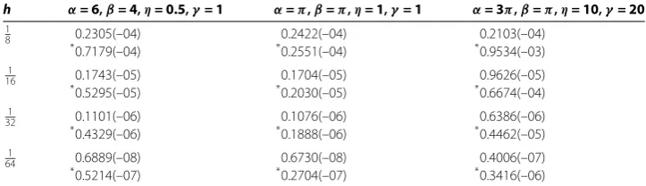
Table 2 Example 2: The maximum absolute errors
h α= 6,β= 4,η= 0.5,γ= 1 α=π,β=π,η= 1,γ= 1 α= 3π,β=π,η= 10,γ= 20
1
8 0.2305(–04) 0.2422(–04) 0.2103(–04)
*0.7179(–04) *0.2551(–04) *0.9534(–03)
1
16 0.1743(–05) 0.1704(–05) 0.9626(–05)
*0.5295(–05) *0.2030(–05) *0.6674(–04)
1
32 0.1101(–06) 0.1076(–06) 0.6386(–06)
*0.4329(–06) *0.1888(–06) *0.4462(–05)
1
64 0.6889(–08) 0.6730(–08) 0.4006(–07)
*0.5214(–07) *0.2704(–07) *0.3416(–06)
*Result obtained by Mohanty [34].
u(,t) = , u(,t) =sinht, t≥. (.c)
We solve equation (.a) using the method (.) in the region bounded by <r< ,t> . The exact solution is given byu(r,t) =rsinht. The maximum absolute errors (MAE) are tabulated in Table att= . and forγ = ,γ = .
Example (Telegraphic equation in general form)
∂u
∂t + (α+β)
∂u
∂t +αβu=c
∂u
∂x +f(x,t), <x< ,t> . (.a)
The initial and boundary conditions are given by
u(x, ) =sinhx, ut(x, ) = –sinhx, ≤x≤, (.b)
u(,t) = , u(,t) =e–tsinh, t≥, (.c) whereα= ,β= ;α=π,β=π, andα= π,β=π. We solve equation (.a) using the method (.). The exact solution is given byu=e–tsinhx. The MAE are tabulated in Ta-ble .
Example (Nonlinear hyperbolic equation)
∂u
∂t =
∂u
∂x +γu
∂u
∂x+
∂u
∂t
+f(x,t), <x< ,t> . (.a)
The initial and boundary conditions are given by
Table 3 Example 3: The maximum absolute errors
h O(k2+h4)-method O(k2+h4)-method
γ= 1 γ= 5 γ= 10 γ= 1 γ= 5 γ= 10
1
8 0.1015(–03) 0.1831(–02) 0.4422(–01) 0.3267(–03) 0.2746(–02) 0.4598(–01) 1
16 0.6438(–05) 0.1080(–03) 0.3198(–02) 0.6032(–04) 0.3570(–03) 0.4750(–02) 1
32 0.4032(–06) 0.6806(–05) 0.1840(–03) 0.1398(–04) 0.6526(–04) 0.8192(–03) 1
64 0.2194(–07) 0.4252(–06) 0.1126(–04) 0.3438(–05) 0.1515(–04) 0.1713(–03)
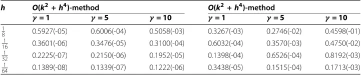
Table 4 Example 4: The maximum absolute errors
h O(k2+h4)-method O(k2+h4)-method
γ= 1 γ= 5 γ= 10 γ= 1 γ= 5 γ= 10
1
8 0.5927(-05) 0.6006(-04) 0.5058(-03) 0.3267(-03) 0.2746(-02) 0.4598(-01) 1
16 0.3601(-06) 0.3476(-05) 0.3100(-04) 0.6032(-04) 0.3570(-03) 0.4750(-02) 1
32 0.2225(-07) 0.2150(-06) 0.1952(-05) 0.1398(-04) 0.6526(-04) 0.8192(-03) 1
64 0.1389(-08) 0.1339(-07) 0.1222(-06) 0.3438(-05) 0.1515(-04) 0.1713(-03)
u(,t) = , u(,t) =sinht, t≥. (.c)
We solve equation (.a) using the method (.) in the region bounded by <x< ,t> . The exact solution is given byu(x,t) =xsinht. The MAE are tabulated in Table for
γ = , and att= ..
Example (Quasi-linear hyperbolic equation)
∂u
∂t =
+x+u∂
u
∂x +γu
∂u
∂x+
∂u
∂t
+f(x,t), <x< ,t> . (.a)
The initial and the boundary conditions are given by
u(x, ) =sinhx, ut(x, ) = –sinhx, ≤x≤, (.b)
u(,t) = , u(,t) =e–tsinh, t≥. (.c) The exact solution is given byu=e–tsinhx. The MAE are tabulated in Table for γ = , and att= .
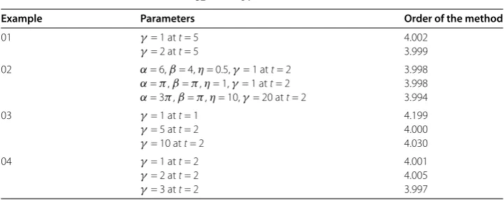
The order of convergence may be obtained by using the formula
log(eh) –log(eh)
log(h) –log(h)
, (.)
whereehandeh are maximum absolute errors for two uniform mesh widthshandh, respectively. For computation of order of convergence of the proposed method, we have consideredh= andh= for all cases, and results are reported in Table .
9 Concluding remarks
Table 5 Order of convergence:h1=321,h2=641
Example Parameters Order of the method
01 γ= 1 att= 5 4.002
γ= 2 att= 5 3.999
02 α= 6,β= 4,η= 0.5,γ= 1 att= 2 3.998 α=π,β=π,η= 1,γ= 1 att= 2 3.998 α= 3π,β=π,η= 10,γ= 20 att= 2 3.994
03 γ= 1 att= 1 4.199
γ= 5 att= 2 4.000
γ= 10 att= 2 4.030
04 γ= 1 att= 2 4.001
γ= 2 att= 2 4.005
γ= 3 att= 2 3.997
three evaluations of the functiong(as compared to five and nine evaluations of the func-tiong discussed in [] and []), we have derived a new stable spline in tension finite difference method ofO(k+h) accuracy for the solution of second-order quasi-linear
hyperbolic equation (.). For a fixed parameterσ=hk, the proposed method behaves like a fourth-order method, which is exhibited by the computed results. The proposed numer-ical method for the wave equation in polar coordinates is conditionally stable, whereas for the damped wave equation and the telegraphic equation, the method is shown to be un-conditionally stable. From Table , we found that the order of the method is nearly equal to four.
Competing interests
The authors declare that they have no competing interest.
Authors’ contributions
RKM derived the difference method based on spline in tension approximation and discussed the convergence analysis of the method. VG has discussed the application of proposed method to wave equation in polar coordinates and telegraphic equation, and stability analysis. VG also carried out all computational work. All authors read and approved the final manuscript.
Author details
1Department of Mathematics, South Asian University, Akbar Bhawan, Chanakyapuri, New Delhi, 110021, India. 2Department of Mathematics, Faculty of Mathematical Sciences, University of Delhi, Delhi, 110007, India.
Acknowledgements
This research work is supported by South Asian University, New Delhi, India. The authors thank the reviewers for their valuable suggestions, which substantially improved the standard of the paper.
Received: 19 November 2012 Accepted: 1 March 2013 Published: 22 March 2013
References
1. Raggett, GF, Wilson, PD: A fully implicit finite difference approximation to the one-dimensional wave equation using a cubic spline technique. IMA J. Appl. Math.14, 75-77 (1974)
2. Fleck, JA Jr.: A cubic spline method for solving the wave equation of nonlinear optics. J. Comput. Phys.16, 324-341 (1974)
3. Fyfe, DJ: The use of cubic splines in the solution of two point boundary value problems. Comput. J.12, 188-192 (1969)
4. Jain, MK, Aziz, T: Spline function approximation for differential equations. Comput. Methods Appl. Mech. Eng.26(2), 129-143 (1981)
5. Jain, MK, Aziz, T: Cubic spline solution of two-point boundary value problems with significant first derivatives. Comput. Methods Appl. Mech. Eng.39(1), 83-91 (1983)
6. Al-Said, EA: Spline methods for solving a system of second order boundary value problems. Int. J. Comput. Math.70, 717-727 (1999)
7. Al-Said, EA: The use of cubic splines in the numerical solution of a system of second order boundary value problem. Comput. Math. Appl.42, 861-869 (2001)
9. Kadalbajoo, MK, Aggarwal, VK: Cubic spline for solving singular two-point boundary value problems. Appl. Math. Comput.156, 249-259 (2004)
10. Kadalbajoo, MK, Bawa, RK: Cubic spline method for a class of non-linear singularly perturbed boundary value problems. J. Optim. Theory Appl.76, 415-428 (1993)
11. Kadalbajoo, MK, Patidar, KC: Tension spline for the numerical solution of singularly perturbed non-linear boundary value problems. Comput. Appl. Math.21(3), 717-742 (2002)
12. Kadalbajoo, MK, Patidar, KC: Tension spline for the solution of self-adjoint singular perturbation problems. Int. J. Comput. Math.79(7), 849-865 (2002)
13. Maruši´c, M: A fourth/second order accurate collocation method for singularly perturbed two-point boundary value problems using tension splines. Numer. Math.88(1), 135-158 (2001)
14. Khan, I, Aziz, T: Tension spline method for second-order singularly perturbed boundary-value problems. Int. J. Comput. Math.82(12), 1547-1553 (2005)
15. Mohanty, RK, Evans, DJ, Arora, U: Convergent spline in tension methods for singularly perturbed two-point singular boundary value problems. Int. J. Comput. Math.82(1), 55-66 (2005)
16. Mohanty, RK, Arora, U: A family of non-uniform mesh tension spline methods for singularly perturbed two-point singular boundary value problems with significant first derivatives. Appl. Math. Comput.172(1), 531-544 (2006) 17. Khan, A, Khan, I, Aziz, T: A survey on parametric spline function approximation. Appl. Math. Comput.171(2), 983-1003
(2005)
18. Kumar, M, Srivastava, PK: Computational techniques for solving differential equations cubic, quintic and sextic splines. Int. J. Comput. Methods Eng. Sci. Mech.10, 108-115 (2009)
19. Rashidinia, J, Jalilian, R, Kazemi, V: Spline methods for the solutions of hyperbolic equations. Appl. Math. Comput.190, 882-886 (2007)
20. Ding, H, Zhang, Y: Parametric spline methods for the solution of hyperbolic equations. Appl. Math. Comput.204, 938-941 (2008)
21. Mohanty, RK, Gopal, V: High accuracy cubic spline finite difference approximation for the solution of one-space dimensional non-linear wave equations. Appl. Math. Comput.218(8), 4234-4244 (2011)
22. Mohanty, RK, Gopal, V: An off-step discretization for the solution of 1D mildly nonlinear wave equations with variable coefficients. J. Adv. Res. Sci. Comput.4(2), 1-13 (2012)
23. Mohanty, RK, Gopal, V: High accuracy arithmetic average type discretization for the solution of two-space dimensional nonlinear wave equations. Int. J. Model. Simul. Sci. Comput.3, 1150005 (2012)
24. Ding, H, Zhang, Y: A new unconditionally stable compact difference scheme ofO(τ2+h4) for the 1D linear
hyperbolic equation. Appl. Math. Comput.207, 236-241 (2009)
25. Ding, H, Zhang, Y, Cao, J, Tian, J: A class of difference scheme for solving telegraph equation by new non-polynomial spline methods. Appl. Math. Comput.218, 4671-4683 (2012)
26. Rashidinia, J, Mohammadi, R: Tension spline approach for the numerical solution of nonlinear Klein-Gordon equation. Comput. Phys. Commun.181(1), 78-91 (2010)
27. Rashidinia, J, Mohammadi, R: Tension spline solution of nonlinear sine-Gordon equation. Numer. Algorithms56(1), 129-142 (2011)
28. Jain, MK: Numerical Solution of Differential Equations, 2nd edn. Wiley, New Delhi (1984) 29. Kelly, CT: Iterative Methods for Linear and Non-Linear Equations. SIAM, Philadelphia (1995) 30. Hageman, LA, Young, DM: Applied Iterative Methods. Dover, New York (2004)
31. Mohanty, RK: Stability interval for explicit difference schemes for multi-dimensional second order hyperbolic equations with significant first order space derivative terms. Appl. Math. Comput.190, 1683-1690 (2007) 32. Varga, RS: Matrix Iterative Analysis, 2nd edn. Springer, Berlin (2000)
33. Mohanty, RK, Jain, MK, George, K: On the use of high order difference methods for the system of one space second order non-linear hyperbolic equations with variable coefficients. J. Comput. Appl. Math.72, 421-431 (1996) 34. Mohanty, RK: New unconditionally stable difference schemes for the solution of multi-dimensional telegraphic
equations. Int. J. Comput. Math.86, 2061-2071 (2009)
35. Mohanty, RK, Arora, U: A new discretization method of order four for the numerical solution of one space dimensional second order quasi-linear hyperbolic equation. Int. J. Math. Educ. Sci. Technol.33, 829-838 (2002)
doi:10.1186/1687-1847-2013-70