R E S E A R C H
Open Access
An exponential B-spline collocation
method for the fractional sub-diffusion
equation
Xiaogang Zhu
*, Yufeng Nie, Zhanbin Yuan, Jungang Wang and Zongze Yang
*Correspondence: [email protected] Department of Applied Mathematics, Northwestern Polytechnical University, Xi’an, 710129, P.R. China
Abstract
In this article, we propose an exponential B-spline approach to obtain approximate solutions for the fractional sub-diffusion equation of Caputo type. The presented method is established via a uniform nodal collocation strategy by using an exponential B-spline based interpolation in conjunction with an effective finite difference scheme in time. The unique solvability is rigorously proved. The
unconditional stability is well illustrated via a procedure closely resembling the classic von Neumann technique. A series of numerical examples are carried out, and by contrast to other algorithms available in the open literature, numerical results confirm the validity and superiority of our method.
Keywords: fractional sub-diffusion equation; exponential B-spline collocation method; unique solvability; unconditional stability
1 Introduction
The basic concept of anomalous diffusion dates back to Richardson’s treatise on atmo-spheric diffusion in []. It has increasingly got recognition since the late s within transport theory. In contrast to a typical diffusion, such a process no longer fol-lows Gaussian statistics, then the classic Fick’s law fails to apply. Its most striking charac-teristic is the temporal power-law pattern dependence of the mean squared displacement [],i.e.,χ(t)∼κtα, for sub-diffusion,α< , whileα> for super-diffusion. Anomalous
transport behavior is ubiquitous in physical scenarios, and due to its universal mutual-ity, formidable challenges are introduced. In recent decades, fractional partial differential equations (PDEs) have entered public vision; they compare favorably with the usual mod-els to characterize such transport motions in heterogeneous aquifer and the medium with fractal geometry [, ]. An explosive interest has been gained to investigate the theoretical properties, analytic techniques, and numerical algorithms for fractional PDEs [–].
As a model problem of the class of fractional PDEs described above, the fractional sub-diffusion equation is considered here
∂αu(x,t)
∂tα –κ
∂u(x,t)
∂x =f(x,t), a≤x≤b, <t≤T, (.)
subjected to the initial and boundary conditions
u(x, ) =ϕ(x), a≤x≤b, (.)
u(a,t) =g(t), u(b,t) =g(t), <t≤T, (.)
where <α< ,κis the positive viscosity constant, andϕ(x),g(t),g(t) are the prescribed
functions with sufficient smoothness. In Eq. (.), the time-fractional derivative is defined in the Caputo sense,i.e.,
∂αu(x,t)
∂tα =
( –α)
t
∂u(x,ξ) ∂ξ
dξ (t–ξ)α,
with Gamma function(·). Problem (.)-(.) describes many natural phenomena and has widely been used in applications such as soft thin films, chemical reactions, optical fiber materials, and wave propagation [–].
There have been some works dedicated to developing numerical algorithms to obtain the solutions of Eqs. (.)-(.) apart from a few analytic techniques that are not always available for general situations. Zhang and Liu derived an implicit difference scheme and proved that it is unconditionally stable []. Yuste and Acedo studied an explicit differ-ence scheme based on the Grünwald-Letnikov formula []. Along the same line, a group of weighted average difference schemes were then obtained []. In [], Cui raised a high-order compact difference scheme and its convergence was detailedly discussed; another similar approach was the compact scheme stated in [] for the fractional sub-diffusion equation with the Neumann boundary condition. In [], an effective spectral method was constructed by using the commonL formula in time and a Legendre spectral ap-proximation in space. Later, this method was extended to the time-space case []. The finite element method was considered by Jiang and Ma []. The semi-discrete lump finite element method was studied by Jinet al. for a time-fractional model with a nonsmooth right-hand function []. Liuet al. described an implicit RBF meshless approach for the time-fractional diffusion equation []. Liet al. suggested an adomian decomposition al-gorithm for the equations of the same type []. In [], the authors solved such equations by employing a fully discrete direct discontinuous Galerkin method. Gaoet al. proposed a new effective difference scheme with the Caputo derivative discretized by theL- for-mula []. Recently, Luoet al. established a quadratic spline collocation method for the fractional sub-diffusion equation [], where the convergence underL∞-norm was ana-lyzed. Sayevandet al. gave a cubic B-spline collocation method [], whose stability was provided. A cubic trigonometric B-spline collocation approach was conducted in [], and a wavelet Galerkin method was studied in []. In [], a Sinc-Haar collocation method which uses the Haar operational matrix to convert the original problem into a set of linear algebraic equations via expanding the approximation as a truncated series based on Sinc and Haar functions was proposed.
tested on five numerical examples and studied in contrast to other algorithms. The pro-posed method is highly accurate and calls for a lower cost to implement. This may make sense to treat the equations as the model we consider here with a long time range. The outline is as follows. In Section , we give a concise description of exponential B-spline trial basis, which will be useful hereinafter. In Section , we construct a fully discrete expo-nential B-spline approach on uniform meshes to discretize the model and prove that it is stable. The initial vector, which we require to start our method, is addressed in Section . To evaluate its accuracy, numerical examples are covered in Section .
2 Description of exponential spline functions
Leta=x<x<x<· · ·<xM–<xM=bbe an equidistant spatial mesh on the interval [a,b], and forM∈Z+, denote
h= (b–a)/M, s=sinh(ph), c=cosh(ph),
The values ofBj(x) andBj(x) at each knot are given as nential spline space on the interval [a,b]. The non-negative freepis termed as ‘tension’ parameter andp→ yields cubic spline, whereasp→ ∞corresponds to the linear spline. The cubic spline interpolation causes extraneous inflexion points, while the exponential splines can produce co-convex interpolation and allow to remedy this issue.
3 An exponential B-spline collocation method
Lettn=nτ,n= , , . . . ,N,T=τN,N∈Z+, andxj=a+jh,j= –, , . . . ,M+,h= (b–a)/M, M∈Z+. On this time-space lattice, we set about deriving the desired exponential B-spline
collocation method for Eqs. (.)-(.).
3.1 Discretization of Caputo derivative
We recall the definitions of fractional derivatives. Given a smooth enoughf(x,t), theαth Caputo derivative is defined by
C
and theαth Riemann-Liouville type derivative is defined by
RL handling the initial-valued problems, and thereby is utilized in time in most instances. (.), (.) interconvert into each other through
C
] for deeper insight. An effective approximation for Caputo derivative can be derived by rewriting Eq. (.) and using proper schemes to discretize (.),i.e.,
with several sets of coefficientsωkq,α,q= , , , , , (see []). Letωα
k =ω
,α
k . Then
ωαk= (–)k
α k
= (k–α)
(–α)(k+ ), k= , , , . . . (.)
in which case the scheme is the one given by Gorenfloet al. []. On imposing <α< , (.) simply reduces to
C
D α
tf(x,tn) = τα
n
k=
ωqk,αf(x,tn–k) – τα
n
k=
ωkq,αf(x, ) +Rq(τ), (.)
with the truncated errorRq(τ) satisfyingRq(τ) =O(τq),q= , , , , .
Lemma . The coefficientsωαk defined in(.)fulfill (a) ωα= ,ωkα< ,∀k≥,
(b) ∞k=ωαk= ,nk=–ωkα> .
Proof See references [, ] for details.
3.2 A fully discrete exponential B-spline based scheme
DefineVM+= span{B–(x),B(x), . . . ,BM(x),BM+(x)}over the interval [a,b] referred to as
an (M+ )-dimensional exponential spline space. Then an approximate solution to Eqs. (.)-(.) is sought onVM+in the form
uN(x,t) = M+
j=–
αj(t)Bj(x), (.)
with the unknown weights{αj(t)}Mj=–+ yet to be determined by some certain restrictions.
Discretizing Eq. (.) by using (.) in time, we have
ωq,αu(x,tn) –τακ ∂u(x,t
n) ∂x
= – n–
k=
ωqk,αu(x,tn–k) + n–
k=
ωkq,αu(x, ) +ταf(x,tn) +ταRq(τ).
Letαnj =αj(tn). On replacingu(x,t) byuN(x,t) and imposing the following collocation and boundary conditions
ωq,αuN(xj,tn) –τακ
∂uN(xj,tn) ∂x
= – n–
k=
ωqk,αuN(xj,tn–k) + n–
k=
ωqk,αuN(xj, ) +ταf(xj,tn),
uN(x,tn) =g(tn), uN(xM,tn) =g(tn),
at each nodal pointxj,j= , , . . . ,M, we obtain
Aαnj–+Aαnj +Aαjn+= – n–
k=
ωqk,αPjn–k+ n–
k=
The unknown weightsαndepend onαn–k,k= , , . . . ,n, at their previous time levels and are found via a recursive style; onceαnis obtained,α–n,αMn+can further be deter-mined with the help of Eqs. (.)-(.). On the other hand, A is an (M+ )×(M+ ) tri-diagonal matrix, therefore the system can be performed by the well-known Thomas algorithm, which simply needs the arithmetic operation costO(M+ ).
4 Initial state
In order to start Eq. (.), an appropriate initial vectorαto the system is required. To this end, we employ the initial conditions
uN(xj, ) =ϕ(xj), j= , , . . . ,M,
together with the collocation constraints
uN(x, ) =ϕ(x), uN(xM, ) =ϕ(xM),
got via Eq. (.) explicitly to determine a unique initial vectorαby
Kα= U (.) Eq. (.) can also be computed by the Thomas algorithm.
5 Stability and solvability
In this section, we prove that Eqs. (.)-(.) with the discrete coefficientsωα
evolves over time, whereZj,Znj–kare the quantities likePj,Pnj–kwith regard to the per-turbation. Since the classic Fourier method does not work for Eq. (.), a fractional von Neumann procedure is employed to analyze its stability.
Lemma . System(.)-(.)is uniquely solvable since its coefficient matricesA, Kare strictly diagonally dominant.
Proof Usingp> and the following Taylor’s expansions
s–ph=(ph)
! + (ph)
! +· · ·+
(ph)k+
(k+ )!+· · ·, (.)
phc–ph=(ph)
! + (ph)
! +· · ·+ (ph)k+
(k)! +· · ·, (.)
it is easy to checks–ph> and another similar inequalityphc–s> by subtracting (.) from (.). In virtue ofA,A, one gets
A– |A|= τακps+ ωα(phc–s) – –τακps+ωα(s–ph) ≥ωα(phc–s) – ωα(s–ph)
= ωα(phc–s) – (s–ph)
since |–τακps+ωα
(s–ph)| ≤τακps+ ωα(s–ph). Then the lemma is ascribed to
s–ph<phc–s. Using (.)-(.) again results in
(phc–ph) – (s–ph) = (ph)
!–
!
+ (ph)
! –
!
+· · ·+ (ph)k+
(k)!–
(k+ )!
+· · ·.
Due to (k)!× < (k)!×(k+ ),k≥, there exist
(phc–s) – (s–ph) = (phc–ph) – (s–ph) > ,
and|A|– |A|> , which implies A is strictly diagonally dominant, so is K. Hence, Eqs. (.)-(.) are uniquely solvable. The proof is completed.
The stability analysis is proceeded as follows.
Theorem . System(.)-(.)is unconditionally stable.
Proof As the usual way, we investigate a single generic modeρjk=ζk
υexp(iυjh) with i =
√
– and the wave numberυ. Inserting it into Eq. (.) yields
Aζυncos(υh) +Aζυn= – n–
k=
ωαkSnυ–k+
n–
k=
where
Sυ= (s–ph)cos(υh)ζυ+ (phc–s)ζυ,
Sυn–k= (s–ph)cos(υh)ζυn–k+ (phc–s)ζυn–k,
by the aid of Euler’s formulaexp(±iυh) =cos(υh)±isin(υh). Noticing that
Acos(υh) +A= τακps –cos(υh)+ ωα(s–ph)cos(υh) + ωα(phc–s), and the inequalities
s–ph> , phc–s> , s–ph<phc–s,
we obtain
ζυn= –
n–
k=
ωαkGζυn–k+
n–
k=
ωαkGζυ (.)
with a non-negative fixed quantity
G= ω
α
(s–ph)cos(υh) +ωα(phc–s)
τακps( –cos(υh)) +ωα
(s–ph)cos(υh) +ωα(phc–s)
not more than . To show|ζυn| ≤ |ζυ|, we use mathematical induction. Asn= , by Eq. (.), we trivially have|ζυ| ≤ |ζυ|sinceωαG≤. Assuming that
ζυm≤ζυ, m= , , . . . ,n– , (.)
it follows from Lemma . that
ζυn≤
–
n–
k=
ωαkGζυn–k+
n–
k=
ωαkGζυ
≤
–
n–
k=
ωαk+ n–
k=
ωαk
G max ≤m≤n–
ζυm
=G max ≤m≤n–
ζυm,
which implies|ζυn| ≤ |ζυ|due toG≤ and the assumptions (.). Hence, we realize that the perturbation remains bounded by its initial perturbation unconditionally at any time
level. This proves what we require.
6 Numerical experiments
In this part, we present a couple of numerical examples so as to gauge the practical perfor-mance of our proposed exponential B-spline collocation method. In the tests, we choose q= except the fifth example. The computing errors are measured by
e(τ,h) =u(x,tn) –uN(x,tn)L=
hM–
j=
u(xj,tn) –uN(xj,tn),
e∞(τ,h) =u(x,tn) –uN(x,tn)L∞= max
Figure 1 The global errors att= 1 for variouspwhenα= 0.9,M= 20, andN= 5,000.
Table 1 The numerical results att= 1 withα= 0.9,p= 5.16, andN= 5,000 for Example 6.1
M u – uNL2 Cov. rate u – uNL∞ Cov. rate
10 8.6951e-4 - 1.3969e-3
-20 2.2384e-4 1.9578 3.6042e-4 1.9545
40 5.7089e-5 1.9712 9.2262e-5 1.9659
80 1.5162e-5 1.9127 2.4710e-5 1.9007
Table 2 The numerical results att= 1 in time withp= 1.52 andM= 300 for Example 6.2
N u – uNL2 Cov. rate u – uNL∞ Cov. rate
10 6.8812e-4 - 9.6064e-4
-20 3.2075e-4 1.1012 4.4793e-4 1.1007
40 1.5101e-4 1.0868 2.1097e-4 1.0862
80 7.1577e-5 1.0771 1.0003e-4 1.0765
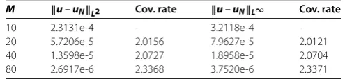
Table 3 The numerical results att= 1 in space withp= 1.52 andN= 5,000 for Example 6.2
M u – uNL2 Cov. rate u – uNL∞ Cov. rate
10 2.3131e-4 - 3.2118e-4
-20 5.7206e-5 2.0156 7.9627e-5 2.0121
40 1.3598e-5 2.0727 1.8958e-5 2.0704
80 2.6917e-6 2.3368 3.7520e-6 2.3371
and lettingν= ,∞, the convergent rates (Cov. rate) are computed by
Cov. rate = ⎧ ⎨ ⎩
log(eν(τ,h)/eν(τ,h))
log(τ/τ) in time,
log(eν(τ,h)/eν(τ,h))
log(h/h) in space.
Figure 2 The exact and numerical solutions att= 1, 3, and 6 whenM= 100 andN= 500.
Table 4 The global errors at different time withp= 0.01 and variousM,Nfor Example 6.3
M,N u – uNL2 u – uNL∞
t = 1 t = 2 t = 3 t = 1 t = 2 t = 3
32, 4,000 5.4324e-5 3.8735e-5 3.1716e-5 8.8587e-5 6.3211e-5 5.1768e-5 64, 4,000 1.3203e-5 9.6132e-6 7.9258e-6 2.1878e-5 1.5795e-5 1.2985e-5 128, 9,000 3.0826e-6 2.3273e-6 1.9418e-6 5.2449e-6 3.8791e-6 3.2140e-6 256, 9,000 5.3117e-7 4.7773e-7 4.2641e-7 9.5837e-7 8.4372e-7 7.3492e-7 1,024, 250 5.9928e-6 2.1116e-6 1.1412e-6 9.4652e-6 3.3298e-6 1.7970e-6 1,024, 500 3.6171e-6 1.2685e-6 6.8189e-7 5.6050e-6 1.9593e-6 1.0500e-6 2,048, 1,000 2.2589e-6 7.9847e-7 4.3255e-7 3.4336e-6 1.2092e-6 6.5273e-7 2,048, 2,000 1.4133e-6 4.9781e-7 2.6867e-7 2.1044e-6 7.3642e-7 3.9486e-7
Example . Leta= ,b= , and the initial boundary conditionsϕ(x) = ,g(t) = , and
g(t) = . The forcing term is given as
f(x,t) = ( +μ) (μ+ –α)t
μ–α
x( –x) – κtμx( – x)
to enforce the exact solutionu(x,t) =tμx( –x). Takingκ= ,α= .,μ= +α, Figure
describes the behavior of the global errors att= versus the variation ofpwithM= andN= ,. As the figure shows, the optimal pfor this problem is roughly located on [., .]. Retakingp= ., Table reports the numerical results att= versus the variation ofMwithN= ,. It is obvious that our method is considerably robust and convergent with second-order in space as the grid is refined.
Example . Recalling the Mittag-Leffler function
Eα(z) =
∞
k=
zk
(αk+ ), <α< ,
endowed withCDα
tEα(–λtα) = –λEα(–λtα) [], we consider Eqs. (.)-(.) on the domain
[, ] with
u(x, ) =sin(πx/), g(t) = , g(t) =Eα
Figure 3 The absolute error distributions for
p= 1.45, 2.35, 2.53, and 3.35 whenM= 50 and
N= 2,500.
and the homogeneous forcing term. It is easy to verify that its exact solution takes the formu(x,t) =Eα(–tα)sin(πx/) whenκ= /π. Lettingα= . andp= ., the numerical
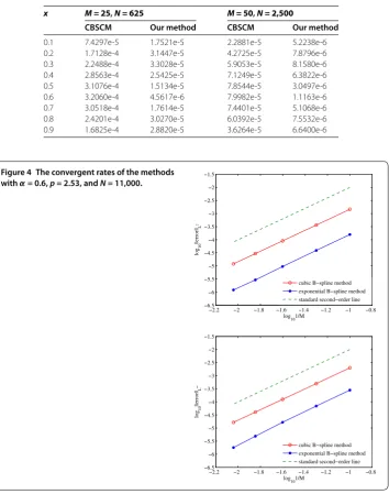
Table 5 The comparison of absolute errors between CBSCM and our method whenp= 2.53
x M = 25,N = 625 M = 50,N = 2,500
CBSCM Our method CBSCM Our method
0.1 7.4297e-5 1.7521e-5 2.2881e-5 5.2238e-6
0.2 1.7128e-4 3.1447e-5 4.2725e-5 7.8796e-6
0.3 2.2488e-4 3.3028e-5 5.9053e-5 8.1580e-6
0.4 2.8563e-4 2.5425e-5 7.1249e-5 6.3822e-6
0.5 3.1076e-4 1.5134e-5 7.8544e-5 3.0497e-6
0.6 3.2060e-4 4.5617e-6 7.9982e-5 1.1163e-6
0.7 3.0518e-4 1.7614e-5 7.4401e-5 5.1068e-6
0.8 2.4201e-4 3.0270e-5 6.0392e-5 7.5532e-6
0.9 1.6825e-4 2.8820e-5 3.6264e-5 6.6400e-6
Figure 4 The convergent rates of the methods withα= 0.6,p= 2.53, andN= 11,000.
results in space with N= , are tabulated in Table , where our method yields the convergent approximations with the desirable accuracy.
Example . In this test, we consider a special case ofα= .. Leta= ,b= ,κ = , ϕ(x) =cos(πx),g(t) = erfcx(π
√
t),g(t) =g(t),f(x,t) = , and the true solution (see
[])
u(x,t) =cos(πx)erfcxπ√t,
whereerfcx(·) is thescaled complementary error functiongiven by
erfcx(z) = √ πexp
z
∞
z
Table 6 The numerical results att= 1 in time withp= 2 andM= 2,000 for Example 6.5
N u – uNL2 Cov. rate u – uNL∞ Cov. rate
q= 2 5 3.5140e-3 - 5.1249e-3
-10 1.0602e-3 1.7288 1.5457e-3 1.7293
20 2.9124e-4 1.8641 4.2449e-4 1.8644
30 1.3357e-4 1.9224 1.9467e-4 1.9227
q= 3 5 1.2790e-3 - 1.8610e-3
-10 1.9799e-4 2.6915 2.8777e-4 2.6931
20 2.7289e-5 2.8590 3.9643e-5 2.8598
30 8.3666e-6 2.9158 1.2150e-5 2.9167
q= 4 5 3.7550e-4 - 5.4383e-4
-10 2.5907e-5 3.8574 3.7487e-5 3.8587
20 1.7273e-6 3.9067 2.4951e-6 3.9092
30 3.7751e-7 3.7506 5.4254e-7 3.7631
Table 7 The numerical results att= 1 in space withp= 2,q= 3, andN= 1,000 for Example 6.5
M u – uNL2 Cov. rate u – uNL∞ Cov. rate
10 1.5963e-3 - 2.2245e-3
-20 3.9985e-4 1.9972 5.5719e-4 1.9973
40 1.0001e-4 1.9993 1.3940e-4 1.9990
80 2.5006e-5 1.9998 3.4874e-5 1.9990
The computation is run withp= .. Figure describes the numerical solutions at differ-ent time compared to the exact solutions whenM= ,N= . As the graph shows, the exact and numerical solutions are in good agreement. Table reports the global errors at t= ,t= , andt= with variousM,N. It is visible that the collocation scheme (.)-(.) well solve the test problem as we expected.
Example . Letκ= ,ϕ(x) = ,g(t) = ,g(t) =g(t), and
f(x,t) = t
–αx( –x)exp(x)
( –α) + t
x(x+ )exp(x);
we consider Eqs. (.)-(.) on the domain [, ] solved by Eqs. (.)-(.) and the cubic B-spline collocation method (CBSCM) []. The exact solution of the model isu(x,t) = tx( –x)exp(x). In Figure , we display their absolute error distributions att= when
α= .,M= ,N= , by takingp= ., ., ., and ., respectively. In line with the graphs, we then choosep= . and show a comparison of their absolute errors at some nodal points detailedly in Table , where the accuracy of our method is found to be overall better than CBSCM. In Figure , we plot the global errors versus the variation of mesh size /Min log-log scale, withα= .,p= ., andN= ,, which demonstrates that the convergent rates of the presented method and CBSCM are all basically of order .
Example . In this test, we consider Eqs. (.)-(.) withκ= and the initial-boundary conditionsϕ(x) =x,g
(t) = , andg(t) = +ton the domain [, ]. The forcing function
is manufactured as
f(x,t) = ( –α)t
–α
Figure 5 The heat flux atx= 0 for variousαwithM= 500 andN= 125.
to enforce the exact solutionu(x,t) = ( +t)x. The algorithm is first performed withα=
.,p= ,q= , , , andM= ,. The numerical results att= in time are tabulated in Table . Then, fixingq= andN= ,, the corresponding results in space are detailedly reported in Table . As seen from these tables, our method can achieve the predicted convergent rates both in time and space.
Example . In the last test, we consider the fractional heat transfer problem on the do-main [, ] withκ= ,ϕ(x) = ,g(t) = , andg(t) =H(t– .) –H(t– .), whereH(·)
denotes the Heaviside step function. As in [], the heat flux at the boundary pointx= approximated by the forward difference is of particular interest, and the computed results are compared with the ones obtained by the implicit finite difference method in the lit-erature. Takingp= ,M= ,N= , Figure exhibits the heat flux atx= changing over the time forα= ., ., and .. It is obvious that the results of these two methods are highly consistent, which reveals that our method precisely captures the heat flux.
7 Conclusion
Acknowledgements
The authors are thankful to the referees for the constructive comments and suggestions. This research was supported by the National Natural Science Foundation of China (Nos. 11471262 and 11501450).
Competing interests
The authors declare that they have no competing interests.
Authors’ contributions
All authors contributed equally to this article. All authors read and approved the final article.
Publisher’s Note
Springer Nature remains neutral with regard to jurisdictional claims in published maps and institutional affiliations.
Received: 24 April 2017 Accepted: 25 August 2017 References
1. Richardson, LF: Atmospheric diffusion shown on a distance-neighbour graph. Proc. R. Soc. A, Math. Phys. Eng. Sci.
110, 709-737 (1926)
2. Metzler, R, Klafter, J: The random walk’s guide to anomalous diffusion: a fractional dynamics approach. Phys. Rep.339, 1-77 (2000)
3. Adams, EE, Gelhar, LW: Field study of dispersion in a heterogeneous aquifer: 2. Spatial moments analysis. Water Resour. Res.28, 3293-3307 (1992)
4. Nigmatullin, RR: The realization of the generalized transfer equation in a medium with fractal geometry. Phys. Status Solidi B133, 425-430 (1986)
5. Barkai, E: CTRW pathways to the fractional diffusion equation. Chem. Phys.284, 13-27 (2002)
6. Deng, WH: Numerical algorithm for the time fractional Fokker-Planck equation. J. Comput. Phys.227(2), 1510-1522 (2007)
7. Gorenflo, R, Mainardi, F: Random walk models for space-fractional diffusion processes. Fract. Calc. Appl. Anal.1, 167-191 (1998)
8. Mainardi, F: The fundamental solutions for the fractional diffusion-wave equation. Appl. Math. Lett.9(6), 23-28 (1996) 9. Meerschaert, MM, Tadjeran, C: Finite difference approximations for fractional advection-dispersion flow equations.
J. Comput. Appl. Math.172, 65-77 (2004)
10. Momani, S, Odibat, Z: Numerical comparison of methods for solving linear differential equations of fractional order. Chaos Solitons Fractals31(5), 1248-1255 (2007)
11. Povstenko, Y: Signaling problem for time-fractional diffusion-wave equation in a half-space in the case of angular symmetry. Nonlinear Dyn.59(4), 593-605 (2010)
12. Zhuang, P, Liu, F, Anh, V, Turner, I: New solution and analytical techniques of the implicit numerical method for the sub-diffusion equation. SIAM J. Numer. Anal.46, 1079-1095 (2008)
13. Datsko, B, Gafiychuk, V, Podlubny, I: Solitary travelling auto-waves in fractional reaction-diffusion systems. Commun. Nonlinear Sci. Numer. Simul.23(1), 378-387 (2015)
14. Kurzke, M: A nonlocal singular perturbation problem with periodic well potential. ESAIM Control Optim. Calc. Var.
12(1), 52-63 (2006)
15. Podlubny, I: Fractional Differential Equations. Academic Press, San Diego (1999)
16. Kilbas, AA, Srivastava, HM, Trujillo, JJ: Theory and Applications of Fractional Differential Equations. Elsevier, Amsterdam (2006)
17. Zhuang, PH, Liu, FW: Implicit difference approximation for the time fractional diffusion equation. J. Comput. Appl. Math.22(3), 87-99 (2006)
18. Yuste, SB, Acedo, L: An explicit finite difference method and a new von Neumann-type stability analysis for fractional diffusion equations. SIAM J. Numer. Anal.42(5), 1862-1874 (2005)
19. Yuste, SB: Weighted average finite difference methods for fractional diffusion equations. J. Comput. Phys.216, 264-274 (2006)
20. Cui, MR: Compact finite difference method for the fractional diffusion equation. J. Comput. Phys.228(20), 7792-7804 (2009)
21. Ren, JC, Sun, ZZ, Zhao, X: Compact difference scheme for the fractional sub-diffusion equation with Neumann boundary conditions. J. Comput. Phys.232(1), 456-467 (2013)
22. Lin, YM, Xu, CJ: Finite difference/spectral approximations for the time-fractional diffusion equation. J. Comput. Phys.
225(2), 1533-1552 (2007)
23. Li, XJ, Xu, CJ: A space-time spectral method for the time fractional diffusion equation. SIAM J. Numer. Anal.47, 2108-2131 (2009)
24. Jiang, YJ, Ma, JT: High-order finite element methods for time-fractional partial differential equations. J. Comput. Appl. Math.235(11), 3285-3290 (2011)
25. Jin, BT, Lazarov, R, Pasciak, J, Zhou, Z: Error analysis of semidiscrete finite element methods for inhomogeneous time-fractional diffusion. IMA J. Numer. Anal.35, 561-582 (2015)
26. Liu, Q, Gu, YT, Zhuang, PH, Liu, FW, Nie, YF: An implicit RBF meshless approach for time fractional diffusion equations. Comput. Mech.48(1), 1-12 (2011)
27. Li, CP, Wang, YH: Numerical algorithm based on Adomian decomposition for fractional differential equations. Comput. Math. Appl.57, 1672-1681 (2009)
28. Huang, CB, Yu, XJ, Wang, C, Li, ZZ, An, N: A numerical method based on fully discrete direct discontinuous Galerkin method for the time fractional diffusion equation. Appl. Math. Comput.264, 483-492 (2015)
30. Luo, WH, Huang, TZ, Wu, GC, Gu, XM: Quadratic spline collocation method for the time fractional subdiffusion equation. Appl. Math. Comput.276, 252-265 (2016)
31. Sayevand, K, Yazdani, A, Arjang, F: Cubic B-spline collocation method and its application for anomalous fractional diffusion equations in transport dynamic systems. J. Vib. Control22, 2173-2186 (2016)
32. Yaseen, M, Abbas, M, Ismail, AI, Nazir, T: A cubic trigonometric B-spline collocation approach for the fractional sub-diffusion equations. Appl. Math. Comput.293, 311-319 (2017)
33. Heydari, MH: Wavelets Galerkin method for the fractional subdiffusion equation. J. Comput. Nonlinear Dyn.11(6), 061014 (2016)
34. Pirkhedri, A, Javadi, HHS: Solving the time-fractional diffusion equation via Sinc-Haar collocation method. Appl. Math. Comput.257, 317-326 (2015)
35. McCartin, BJ: Theory, computation, and application of exponential splines. Courant Mathematics and Computing Laboratory Research and Development Report DOE/ER/03077-171, New York (1981)
36. McCartin, BJ: Theory of exponential splines. J. Approx. Theory66(1), 1-23 (1991)
37. Chen, MH, Deng, WH: Fourth order difference approximations for space Riemann-Liouville derivatives based on weighted and shifted Lubich difference operators. Commun. Comput. Phys.16(2), 516-540 (2014)
38. Gorenflo, R, Mainardi, F, Moretti, D, Paradisi, P: Time fractional diffusion: a discrete random walk approach. Nonlinear Dyn.29(1-4), 129-143 (2002)
39. Deng, WH, Chen, MH, Barkai, E: Numerical algorithms for the forward and backward fractional Feynman-Kac equations. J. Sci. Comput.62(3), 718-746 (2015)
40. Brunner, H, Ling, L, Yamamoto, M: Numerical simulations of 2D fractional subdiffusion problems. J. Comput. Phys.
229(18), 6613-6622 (2010)