R E S E A R C H
Open Access
Efficient solutions of systems of fractional
PDEs by the differential transform method
Aydin Secer
1*, Mehmet Ali Akinlar
2and Adem Cevikel
3*Correspondence:
1Department of Mathematical
Engineering, Faculty of Chemical and Metallurgical Eng., Yildiz Technical University, 34210 Davutpasa, Istanbul, Turkey Full list of author information is available at the end of the article
Abstract
In this paper we obtain approximate analytical solutions of systems of nonlinear fractional partial differential equations (FPDEs) by using the two-dimensional differential transform method (DTM). DTM is a numerical solution technique that is based on the Taylor series expansion which constructs an analytical solution in the form of a polynomial. The traditional higher order Taylor series method requires symbolic computation. However, DTM obtains a polynomial series solution by means of an iterative procedure. The fractional derivatives are described in the Caputo fractional derivative sense. The solutions are obtained in the form of rapidly
convergent infinite series with easily computable terms. DTM is compared with some other numerical methods. Computational results reveal that DTM is a highly effective scheme for obtaining approximate analytical solutions of systems of linear and nonlinear FPDEs and offers significant advantages over other numerical methods in terms of its straightforward applicability, computational efficiency, and accuracy.
Keywords: fractional differential equation; Caputo fractional derivative; differential transform method
1 Introduction
Mathematical modeling of many physical systems leads to linear and nonlinear fractional differential equations in various fields of physics and engineering. For the last several decades, fractional calculus has found diverse applications in various scientific and tech-nological fields such as control theory, computational fluid mechanics, signal and image processing, and many other physical processes (see, for instance, [] for further applica-tions).
The numerical and analytical approximations of FPDEs and systems of FPDEs have been an active research area for computational scientists since the work of Padovan []. Recently, several mathematical methods including the Adomian decomposition (ADM) [], variational iteration (VIM) [], differential transform [], and homotopy perturbation (HAM) [] have been developed to obtain exact and approximate analytic solutions of FPDEs. Some of these methods use some sort of transformations in order to reduce equa-tions into simpler equaequa-tions or systems of equaequa-tions, and some other methods express the solution in a series form which converges to the exact solution. For instance, VIM and ADM provide immediate and visible symbolic terms of analytic solutions as well as nu-merical approximate solutions to both linear and nonlinear differential equations without linearization or discretization.
In this paper we use DTM to obtain approximate analytical solutions of systems of non-linear FPDEs. DTM was not often applied to the solution of systems of nonnon-linear fractional partial differential equations in the literature. DTM is a numerical solution technique that is based on the Taylor series expansion which constructs an analytical solution in the form of a polynomial. The traditional high order Taylor series method requires symbolic com-putation. However, DTM obtains a polynomial series solution by means of an iterative procedure. DTM was first applied in the engineering domain in []. Recently, the appli-cation of DTM was successfully extended to obtain analytical approximate solutions to linear and nonlinear ordinary differential equations of fractional order [, ]. The fact that DTM solves nonlinear equations without using Adomian polynomials can be considered as an advantage of this method over the Adomian decomposition method. A comparison between DTM and the Adomian decomposition method for solving fractional differential equations is given in []. Further applications of DTM might be seen at [, ].
Organization of this paper is as follows. Section overviews fractional calculus briefly and provides some basic definitions and properties of fractional calculus theory. Section describes the generalized two-dimensional DTM. In the same section, several numerical experiments as the application of DTM to some linear and nonlinear systems of FPDEs are presented. Comparison of DTM with HAM and VIM is studied in the final part of the paper.
2 Fractional calculus
There are several different definitions of the concept of a fractional derivative []. Some of these are Riemann-Liouville, Grunwald-Letnikow, Caputo, and generalized functions approach. The most commonly used definitions are the Riemann-Liouville and Caputo derivatives.
Definition . A real functionf(x),x> , is said to be in the space Cμ,μ∈R, if there exists a real numberp(>μ) such thatf(x) =xpf(x), wheref(x)∈C[,∞), and it is said to be in the spaceCm
μ ifffm∈Cμ,m∈N.
Definition . The Riemann-Liouville fractional integral operator of orderα≥ of a functionf ∈Cμ,μ≥–, is defined as
Jvf(x) =
(v)
x
(x–t)v–f(t)dt, v> ,
Jf(x) =f(x).
It has the following properties. Forf∈Cμ,μ≥–,α,β≥, andγ> :
. JαJβf(x) =Jα+βf(x),
. JαJβf(x) =JβJαf(x),
. Jαxγ= (γ + )
(α+γ+ )x
α+γ
.
defi-nition of fractional order initial conditions which have no physically meaningful explana-tion yet. Caputo introduced an alternative definiexplana-tion which has the advantage of defining integer order initial conditions for fractional order differential equations.
Definition . The fractional derivative off(x) in the Caputo sense is defined as
D*vf(x) =Jam–vDmf(x) =
(m–v)
x
(x–t)m–v–f(m)(t)dt,
form– <v<m,m∈N,x> ,f ∈C–m.
Lemma . If m– <α<m,m∈N,and f ∈Cm
μ,μ≥–,then
Dα
*Jαf(x) =f(x),
JαDv
*f(x) =f(x) –
m–
k=
fk+x
k
k!, x> .
The Caputo fractional derivative is considered here because it allows traditional initial and boundary conditions to be included in the formulation of the problem.In this paper,we have considered some systems of linear and nonlinear FPDEs,where fractional derivatives are taken in Caputo sense as follows.
Definition . Formto be the smallest integer that exceedsα, the Caputo time-fractional derivative operator of orderα> is defined as
Dα*tu(x,t) =∂
αu(x,t)
∂tα =
⎧ ⎨ ⎩
(m–α)
t
(t–ξ)
m–α–∂mu(x,ξ)
∂ξm dξ, form– <α<m,
∂mu(x,t)
∂tm , forα=m∈N.
3 Generalized two-dimensional DTM
In this section we shall derive the generalized two-dimensional DTM that we have de-veloped for the numerical solution of linear partial differential equations with space and time-fractional derivatives.
Consider a function of two variablesu(x,y) and suppose that it can be represented as a product of two single-variable functions,i.e.,u(x,y) =f(x)g(y). Based on the properties of the generalized two-dimensional differential transform, the functionu(x,y) can be repre-sented as
u(x,y) =
∞
k=
Fα(k)(x–x)kα
∞
h=
Gβ(h)(y–y)hβ
=
∞
k=
∞
h=
Uαβ(k,h)(x–x)kα(y–y)hβ,
where <α,β≤,Uαβ(k,h) =Fα(k)Gβ(h) is called the spectrum ofu(x,y). The general-ized two-dimensional differential transform of the functionu(x,y) is given by
Uα,β(k,h) =
(αk+ )(βh+ )
Dα*xkDβ*yhu(x,y)(x
where (Dα x)
k=Dα xD
α x· · ·D
α
x,k-times. In case ofα= andβ= , the generalized
two-dimensional differential transform () reduces to the classical two-two-dimensional differential transform. Next we give some useful theorems about writing the generalized differential transform in equivalent forms under certain conditions.
Theorem .[] Suppose that Uα,β(k,h),Vα,β(k,h),and Wα,β(k,h)are the differential transformations of the functions u(x,y),v(x,y),and w(x,y),respectively,then
ifu(x,y) =v(x,y)±w(x,y),thenUα,β(k,h) =Vα,β(k,h)±Wα,β(k,h), ifu(x,y) =av(x,y),a∈R,thenUα,β(k,h) =aVα,β(k,h),
ifu(x,y) =v(x,y)w(x,y),thenUα,β(k,h) =
k r=
h
s=Vα,β(r,h–s)Wα,β(k–r,s), ifu(x,y) = (x–x)nα(y–y)mβ,thenUα
,β(k,h) =δ(k–n)δ(h–m).
Theorem .[] If u(x,y) =Dα
xv(x,y), <α≤,then the generalized differential trans-form()can be written as
Uα,β(k,h) =
(α(k+ ) + )
(αk+ ) Vα,β(k+ ,h).
Theorem .[] Assume that u(x,y) =f(x)g(y)and the function f(x) =xλh(x),whereλ>
–and h(x)has the generalized Taylor series expansion h(x) =∞n=an(x–x)αk.If (a) β<λ+ andαis arbitrary or
(b) β≥λ+ andαis arbitrary andan= forn= , , . . . ,m– ,wherem– <β≤m. Then the generalized differential transform()becomes
Uα,β(k,h) =
(αk+ )(βh+ )
Dα*xkDβ*yhu(x,y)(x
,y).
Theorem .[] If u(x,y) =Dγxv(x,y), m– <γ ≤m and v(x,y) =f(x)g(y),then the generalized differential transform()can be written as
Uα,β(k,h) =
(αk+γ + )
(αk+ ) Vα,β(k+γ/α,h).
In the next section,we apply DTM to some systems of FPDEs which might have applications in mathematical biology and computational chemistry.
4 Analytical solutions of systems of linear and nonlinear FPDEs
Example Consider the following system of linear FPDEs. For ( <α,β< ),
Dα*tu–vx+ (u+v) = ,
Dβ*tv–ux+ (u+v) = ,
with initial conditionsu(x, ) =sinhxandv(x, ) =coshx. Using DTM, we can write
(α(h+ ) + )
(αh+ ) U(k,h+ ) = (k+ )V(k+ ,h) –U(k,h) –V(k,h),
(β(h+ ) + )
(βh+ ) V(k,h+ ) = (h+ )U(k,h+ ) –U(k,h) –V(k,h).
The transformed initial conditions are
Substituting () in (), we get the following closed form solutions:
u(x,t) =sinh(x)
which are exactly the same as the solutions obtained by HAM converging to the closed-form solutions:
u(x,t) =sinh(x–t),
v(x,t) =cosh(x–t).
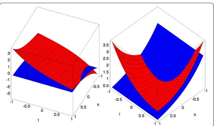
Forα=β= , Figure illustrates exact and approximate solutions obtained by DTM of
u(x,t) andv(x,t), respectively.
Example Consider the following nonlinear system. For ( <α,β< ),
Figure 1 Forα=β= 1: exact and approximate solutions (red and blue colored surfaces, respectively) (u(x,t) andv(x,t) (left- and right-hand sides, respectively)).
(β(h+ ) + )
(βh+ ) V(k,h+ ) = (k+ )(k+ )V(k+ ,h) +
k
r=
h
s=
V(r,h–s)(k–r+ )
×V(k–r+ ,s) –
k
r=
h
s=
(r+ )U(r+ ,h–s)V(k–r,s)
–
k
r=
h
s=
(r+ )V(r+ ,h–s)U(k–r,s). ()
The transformed version of the initial conditions is
U(k, ) =V(k, ) =
⎧ ⎪ ⎪ ⎨ ⎪ ⎪ ⎩
, k= , , , . . . ,
k!, k= , , . . . , –
k!, k= , , . . . .
()
Substituting () in () and (), we obtained the following closed form solutions:
u(x,t) =
x
!–
x ! +· · ·
+
∞
m=
(–tα)m (mα+ )
,
v(x,t) =
x
!–
x ! +· · ·
+
∞
m=
(–tα)m (mα+ )
.
Ifα=β= , we getu(x,t) =sinxe–t, v(x,t) =sinxe–t, which are the exact solutions of the system of equations ().
5 Conclusion and discussion
In this work, the differential transform method is extended to solve linear and non-linear systems of fractional partial differential equations. The present study has confirmed that DTM offers significant advantages in terms of its straightforward applicability, computa-tional efficiency, and accuracy.
Competing interests
The authors declare that they have no competing interests.
Authors’ contributions
The idea of applying the differential transform method (DTM) to the systems of fractional partial differential equations (FPDE) came up as a result of a sequence of scientific discussions by the authors. We, the authors, all together, realized that the DTM has not often been applied to the system of FPDEs in the literature. In particular, AS suggested to applying derivative in the Caputo fractional derivative sense which is different from other fractional derivatives. MAA made a literature search about the related work and tried to found the useful theorems about the subject. AS and AC applied the DTM to some systems of FPDEs. AS implemented the solution algorithm in the Maple programming language. Finally, the authors interpreted the results all together.
Author details
1Department of Mathematical Engineering, Faculty of Chemical and Metallurgical Eng., Yildiz Technical University, 34210
Davutpasa, Istanbul, Turkey.2Department of Mathematics, Faculty of Art and Sciences, Bilecik Seyh Edebali University,
Bilecik, 11210, Turkey. 3Department of Mathematics, Faculty of Art and Sciences, Yildiz Technical University, 34210
Davutpasa, Istanbul, Turkey.
Received: 4 October 2012 Accepted: 19 October 2012 Published: 2 November 2012 References
1. Hilfer, R (ed.): Applications of Fractional Calculus in Physics. Academic Press, Orlando (1999)
2. Padovan, J: Computational algorithms for FE formulations involving fractional operators. Comput. Mech.5, 271-287 (1987)
3. Wu, L, Xie, L, Zhang, J: Adomian decomposition method for nonlinear differential-difference equations. Commun. Nonlinear Sci. Numer. Simul.14(1), 12-18 (2009)
4. Odibat, Z, Momani, S: Application of variational iteration method to nonlinear differential equations of fractional order. Int. J. Nonlinear Sci. Numer. Simul.7(1), 15-27 (2006)
5. Zhou, JK: Differential Transformation and Its Applications for Electrical Circuits. Huazhong University Press, Wuhan, China (1986)
6. Xu, H, Liao, S, You, X: Analysis of nonlinear fractional partial differential equations with the homotopy analysis method. Commun. Nonlinear Sci. Numer. Simul.14(4), 1152-1156 (2009)
7. Ma, S, Xu, Y, Yue, W: Existence and uniqueness of solution for a class of nonlinear fractional differential equations. Adv. Differ. Equ.2012, 133 (2012). doi:10.1186/1687-1847-2012-133
8. Khan, NA, Jamil, M, Ara, A, Khan, N-U: On efficient method for system of fractional differential equations. Adv. Differ. Equ.2011, 303472 (2011). doi:10.1155/2011/303472
9. Arikoglu, A, Ozkol, I: Solution of fractional differential equations by using differential transform method. Chaos Solitons Fractals34, 1473-1481 (2007)
10. Momani, S, Odibat, Z, Erturk, V: Generalized differential transform method for solving a space and time fractional diffusion-wave equation. Phys. Lett. A370(5-6), 379-387 (2007)
11. Ravi Kanth, ASV, Aruna, K: Differential transform method for solving linear and non-linear systems of partial differential equations. Phys. Lett. A, (2008). doi:10.1016/j.physleta.2008.10.008
12. Podlubny, I: Fractional Differential Equations. An Introduction to Fractional Derivatives, Fractional Differential Equations, Some Methods of Their Solution and Some of Their Applications. Academic Press, San Diego (1999) 13. Jafari, H, Seifi, S: Solving a systems of nonlinear fractional partial differential equations using homotopy analysis
method. Commun. Nonlinear Sci. Numer. Simul.14, 1962-1969 (2009)
doi:10.1186/1687-1847-2012-188