R E S E A R C H
Open Access
Jacobi orthogonal approximation with
negative integer and its application to
ordinary differential equations
Xiao-yong Zhang
1and Zheng-su Wan
2**Correspondence: [email protected] 2Department of Mathematics,
Hunan Institute of Science and Technology, Yueyang, 414006, China
Full list of author information is available at the end of the article
Abstract
In this paper, the Jacobi spectral method for ordinary differential equations, which is based on the Jacobi approximation with negative integer, is proposed. This method is very efficient for the initial value problem of ordinary differential equations. The global convergence of proposed algorithm is proved. Numerical results demonstrate the spectral accuracy of this new approach and coincide well with theoretical analysis.
MSC: 35Q99; 35R35; 65M12; 65M70
Keywords: Jacobi approximation with negative integer; spectral method; ordinary differential equation
1 Introduction
Many practical problems arising in science and engineering require us to solve the initial value problems of first-order ODEs. There have been fruitful results on their numerical solutions (see,e.g., Butcher [, ], Haireret al.[], Hairer and Wanner [], Higham [] and Stuart and Humphries []). For Hamiltonian systems, we refer to the powerful symplectic difference method of Feng [], also see [, ] and the references therein.
In the past four decades, the spectral-collocation algorithm has been developed rapidly [–]. Compared with the finite-difference method, its merit is high accuracy. But the main approach used there is the spectral-collocation method which is similar to the finite-difference approach. It makes use of values of interpolation points to present coefficients of expanded form of the numerical solution, and as a result its computing scheme is com-plex and the corresponding error analysis is tedious. However, with a finite-element type approach, as shown in this paper, it is natural to put the approximation scheme under the general inner product type framework. We take advantage of the property of orthogo-nal polynomials sufficiently, and the results are that the computing scheme is simple and that the relevant convergence theory, as will be seen from Section , is cleaner and more reasonable than the collocation method.
In this paper, a kind of novel algorithm, which is called Jacobi spectral method, is pro-posed to solve the initial value problem of the equationdu
dx=f(u,x), and it differs from the
collocation method and has several advantages. Firstly, although both the spectral method and the collocation algorithm possess high accuracy, the spectral method is simpler in
computing scheme and easier to be implemented, especially for nonlinear systems. Sec-ondly, compared with the difference method, the spectral method possesses high accuracy. Finally, the numerical solution is represented in the form of continuous function, so it can more entirely simulate the global property of exact solution and provide more information about the structures of exact solution than the collocation algorithm. Sometimes, this is very important in many practical problems. Theoretical analysis of the spectral method is simpler than that of the collocation method.
The paper is organized as follows. In the next section, we investigate the Jacobi approx-imation. In Section , we propose a kind of new algorithm by using the Jacobi approxima-tion with negative integer. We present numerical results in Secapproxima-tion , which demonstrate the spectral accuracy of the proposed method and coincide well with the theoretical anal-ysis. The final section is conclusion.
2 Orthogonal approximation
In this section, we investigate some results about the Jacobi approximation. Let={x| – <x< }andχ(α,β)(x) = ( –x)α( +x)β,α,β> – be a certain weight function. We define
the weighted space
Lχ(α,β)() =
v|vis measurable onandvχ(α,β)<∞
,
with the following inner product and norm:
(u,v)χ(α,β)=
u(x)v(x)χ(α,β)(x)dx, vχ(α,β)= (v,v) χ(α,β).
For any integerm≥, we define the weighted Sobolev space
Hχm(α,β)() =
vd
kv
dxk ∈L
χ(α,β)(), ≤k≤m
,
equipped with the following inner product, semi-norm and norm:
(u,v)m,χ(α,β)=
≤k≤m
dku
dxk,
dkv
dxk
χ(α,β) ,
|v|m,χ(α,β)=
ddxmmv
χ(α,β)
, vm,χ(α,β)= (v,v)/ m,χ(α,β). For anyr> , the spaceHr
χ(α,β)() and its normvr,χ(α,β)are defined by space interpolation as in []. In particular,Hχ(α,β)() ={v∈Hχ(α,β)()|v(–) = }.
Letχ(α,β)(x) = ( –x)α( +x)β,α,β> –. The Jacobi polynomials of degreelare defined
by
( –x)α( +x)βJ(α,β)
l (x) =
(–)l
ll!
dl
dxl
( –x)l+α( +x)l+β, l= , , , . . . .
They are the eigenfunctions of the Sturm-Liouville problem
d
dx ( –x)
+α( +x)+βdv(x)
dx
with the corresponding eigenvaluesλ(lα,β)=l(l+α+β+ ). They fulfill the following
re-Now, letNbe any positive integer andPN() be the set of all algebraic polynomials of
degree at mostN. Furthermore,PN() ={v∈PN()|v(–) = }.
For any realr> , we define the spaceHr
χ(α,β),A() and its norm by space interpolation as in [].
We also define the spaceHχr(α,β),A() as
Hχr(α,β),A() =
v∈Hχr(α,β),A()|v(–) =
.
For any realγ,δ> –, similar toL
χ(α,β)(), we define the spaceLχ(γ,δ)(). In forthcoming discussions, we will use the following lemma.
Lemma . If
<α≤γ+ , <β≤δ+ ,
then for any v∈H
χ(α,β)()∩Lχ(γ,δ)(), vχ(γ,δ)≤cv,χ(α,β).
Moreover,for any v∈Hχ(α,β)()∩Lχ(γ,δ)()with v(x) = ,x∈,
vχ(γ,δ)≤c|v|,χ(α,β)
provided that
α≤γ + , β≤δ+ .
For the proof, see Lemma . of [].
Next, we recall the Jacobi orthogonal approximation. The orthogonal projectionPN,α,β:
L
χ(α,β)()→PN() is defined by
(PN,α,βv–v,φ)χ(α,β)= , ∀φ∈PN().
We also define the projectionPN,α,β:Lχ(α,β)()→PN() as
(PN,α,βv–v,φ)χ(α,β)= , ∀φ∈PN(),
where
Lχ(α,β)() =
v|v∈Lχ(α,β)() andv(–) =
.
The following results characterize the property ofPN,α,βandPN,α,β. Lemma . For any integers r≥,v∈Hr
χ(α,β),A()∩Lχ(α,β)(), PN,α,βv–vχ(α,β)≤cN–rvr,χ(α,β),A.
Lemma . For any integers r≥,v∈Hχr(α,β),A()∩Lχ(α,β)(), PN,α,βv–vχ(α,β)≤cN–rvr,χ(α,β),A.
Proof By the projection theorem,
PN,α,βv–vχ(α,β)≤ φ–vχ(α,β), ∀φ∈PN().
Takeφ(x) =–x PN–,α,βvdξ in the above. Clearly,φ∈PN(). According to Lemma .,
we have
PN,α,βv–vχ(α,β)≤c
PN–,α,β
dv dx–
dv dx
χ(α,β) .
A combination of Lemma . and this inequality leads to the desired result.
Lemma . For anyφ∈PN()∩Hχr(α,β)()∩Lχ(α,β)(),integer r≥, φ
r,χ(α,β)≤cNrφχ(α,β). For the proof, see [].
For numerical solutions of ordinary differential equations, we need other orthogonal projections. For this purpose, we introduce the space, forr≥n,
Hr
,n() =
v|vis measurable onandvHr
,n,<∞
,
equipped with the following semi-norm and norm:
|v|Hr
,n()=
ddxrvr
χ(r,–n+r)
, vHr
,n()=
r
k=
|v|Hk
,n()
.
Accordingly, we define the space, forr≥n,
Hr,n() =
φ∈Hr,n()d
lφ(–)
dxl = , ≤l≤n–
.
In this paper, we shall use a specific family of Jacobi polynomials. They are defined by
L(,n)
l (x) = ( +x) nJ(,n)
l–n (x), l≥n,n≥.
The set ofL(,l n)(x) is the completeL
χ(,–n)()-orthogonal system, namely
L(,n)
l ,L(,mn)
χ(,–n),=
γm(,–nn), l=m,
, l=m. (.)
Let
PNn() =
φ∈PN()
dlφ(–)
dxl = , ≤l≤n–
Now we define the projection operatorPNn,:H,rn()→PNn() as
–
dn(v–Pn,
N v)
dxn
dnφ
dxnχ
(n,)dx= , ∀φ∈
PNn(). Lemma . For any v∈Hr,n(),integer≤k≤r≤N+ ,
dxdkk
v–PNn,v
χ(k,–n+k)≤
cNk–rdrv
dxr
χ(r,–n+r) .
For the proof, see Lemma . of []. Next, we introduce a polynomial
χn–(x) =
n–
l=
dlϕ(–)
dxl
( +x)l
l! ∈PN(),
which satisfies
dmχ–
n(–)
dxm =
dmϕ(–)
dxm , ≤m≤n– .
For each functionϕinHr
,n(), we define a functionϕ˜ninHr,n() by ˜
ϕn=ϕ–χn–(x). (.)
Following the same idea as in [], we define the Jacobi quasi-orthogonal projection as
Pn,Nϕ=PnN,ϕ˜n+χn–(x). (.)
Obviously, for anyϕ∈Hχr(r,–n+r)() and integerr≥k≥,
ϕ–Pn,Nϕ=ϕ˜n–PNn,ϕ˜n.
Using Lemma . leads to
dxdkk
ϕ–Pn,Nϕ
χ(k,–n+k) =d
k
dxk
˜
ϕn–PnN,ϕ˜n χ(k,–n+k)
≤cNk–rd
rϕ
dxr
χ(r,–n+r)
. (.)
Next, we defineP
N as
PNϕ=PN,α,βϕ˜+ϕ(–). (.)
By using Lemma ., for anyϕ∈Hr
χ(α,β),A()∩Lχ(α,β)(), we obtain
3 Jacobi spectral method with negative integer
In this section, we apply Jacobi approximation with negative integer to ordinary differen-tial equation.
First, we introduce Jacobi polynomials of degreelwith negative integer
L(,)
l (x) = ( +x)J
(,)
l– (x), l= , , . . . . (.)
The set ofL(,)l (x) is the completeL
χ,–()-orthogonal system, namely
L(,)
l ,L
(,)
m
χ,–,=
γl(,)– , l=m,
, l=m. (.)
Obviously,
PN() =span
L(,) ,L
(,) , . . . ,L
(,)
N
. (.)
Next, we define the projectionPN,,–:Lχ(,–)()→PN() as
(PN,,–u–u,φ)χ,–= , ∀φ∈PN().
About this projection, we have the following theorem.
Theorem . If u∈Lχ(,–)()andd
ru
dxr ∈Lχ(r,–+r)(),integers≤r≤N+ , PN,,–u–uχ(,–)≤cN–r
ddxrur
χ(r,–+r) .
The proof is similar to Lemma . of []. Next, we consider the following problem:
dw
dt =f(w(t),t), <t≤T,
w() =v.
For the sake of applying the theory of orthogonal polynomials conveniently, by the linear transformation,
t=T( +x)
, v(x) =w
T( +x)
,
then
dv
dx=f(v(x),x), – <x≤,
v(–) =v.
Letu=v–v,
du
dx=f(u(x) +v,x), – <x≤,
Next, we construct the numerical scheme. To do this, we approximateu(x) byuN(x), where
Due to the orthogonality ofL(,)l , we deduce that
( +x)d
We derive the following spectral scheme for (.)
ANuN=FNuN. (.)
Obviously, system (.) is equivalent to
By the definition ofPN,,–, we obtain that
( +x)duN(x)
dx =PN,,–( +x)f(uN(x) +v,x), x≥–,
uN(–) = .
Remark . In Section , we will see that the global errors decay exponentially asN in (.) increases.
Next, we analyze the numerical error of (.). To do this, letEN =uN–PNu. We suppose
that dudx is continuous forx≥–. Let
G=
d dxP
Nu(x) –PN
du
dx. (.)
Then we have that
d dxP
Nu(x),φ
χ(,)
= PNdu dx,φ
+ (G,φ)χ(,), ∀φ∈PN()χ(,). (.)
Subtracting (.) from (.) yields that
(dxdEN(x),φ)χ(,)= (G,φ)χ(,)– (G,φ)χ(,), ∀φ∈PN(),
EN(–) = ,
(.)
where
G=f
uN(x) +v,x
–PNdu
dx and EN(x)∈PN(). Takingφ= EN in (.) leads to
EN,
d dxEN
χ(,)
= (G,EN)χ(,)– (G,EN)χ(,)
=A+A, (.)
where
A= –(G,EN) and A= (G,EN).
SinceEN(–) = , integration by parts yields
EN,
d dxEN
χ(,)
=EN(+)
. (.)
By using the Cauchy inequality, we derive that
|A| ≤Gχ(,)ENχ(,)≤εENχ(,)+
εG
Next, we assume that there exists a real numberγ such that
According to the above formula, we obtain that
A≤–γENχ(,)+ γPNu–uχ(,)ENχ(,)+
Substituting (.), (.), (.) into (.), we assert that
EN(+)
With the aid of the above formula, we obtain that
(γ– ε)ENχ(,) ≤c PNu–u
By virtue of Lemma ., we derive that
PNu–P,Nu,χ(,) ≤cNPNu–P,Nu
Theorem . If u belongs to Hr
χ(,),A()and dru
dxr belongs to Lχ(r,–+r)(),then,by(.)and (.),
ENχ,≤cN–r
du dx
r,χ(,),A +d
u
dx
r,χ(,),A
+cN–rd
ru
dxr
χ(r,–+r) .
Remark . Assume that for a certain real numberγsuch that
f(z,x) –f(z,x)
(z–z)≤γ(z–z) (.)
the algorithm is still applicable. In this case, we takeαsuch thatγ–α= –γ < and make
the variable transformation
u(x) =eαxU(x), FU(x),x=e–αxfeαxU(x),x–αU(x),
dU(x)
dx =F(U(x),x), x> –,
U(–) = .
(.)
We may use (.) to resolve (.) and obtain the numerical solutionUN(x). Moreover,
condition (.) ensures the global accuracy ofUN(x). The numerical solution of (.) is
given byuN(x) =eαxUN(x).
Remark . The proposed method is also available for solving systems of first-order ODEs. In this case, let
u(x) =u()(x),u()(x), . . . ,u(m)(x),
fu(x),x=f()(u,x),f()(u,x), . . . ,f(m)(u,x).
We consider the system
d
u(x)
dx =f(u(x),x), x> –,
u(–) = . (.)
We approximateubyuN.We can derive a numerical algorithm which is similar. Further,
let be|v|Ethe Euclidean norm ofv. Assume that
f(z,x) –f(z,x)
(z–z)≤–γ|z–z|E.
Then we can obtain an error estimate similar to Theorem ..
4 Numerical results
In this section, we present some numerical results. We first use scheme (.) to solve the problem
du dx= –
u(x)
+F(x), x≥–,
u(–) =u–,
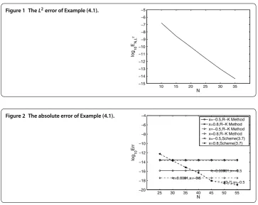
Figure 1 TheL2error of Example (4.1).
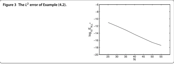
Figure 2 The absolute error of Example (4.1).
which fulfills condition (.) withγ = – . Take the test functionu(x) =cos(x)(x+ ).
Then a direct computation shows that
F(x) = cos(x)(x+ )–sin(x)(x+ )+
cos(x)(x+ )
.
For description of numerical errors, we introduce the global errorEN,L=uN–u and
the absolute error Err =|uN(x) –u(x)|.
In Figure , we plot the global errorslogofEN with various values ofN. They indicate
that the global errors decay exponentially asN increases. They coincide very well with theoretical analysis.
In Figure , we compare scheme (.) with the classical four-stage explicit Runge-Kutta methods for Example (.) withτ= .,τ= .. We find that the method (.) is more accurate than the Runge-Kutta methods for largeN.
We next use scheme (.) to solve the problem
dv dx=
exp(cos(v(x))) +F(x), x≥–,
v(–) =v,
which fulfills condition (.) withγ=e. In this case, we takeα=e such thatγ–α=
–γ = –e < and make the variable transformation
v(x) =eexu(x), fu(x),x=e–ex exp
coseexu(x)+F(x)
–e u(x),
du(x)
dx =f(u(x),x), x> –,
which fulfills condition (.) with –γ = –e. Take the test functionv(x) =e–x(x+ ). Then
a direct computation shows that
F(x) = e–x(x+ )–e–x(x+ )– exp
cose–x(x+ ). Obviously,f(u,x) is a nonlinear function foru. Let
u(Nm)(x) =
N
l=
˜
u(lm)L(,)l ,
then
(dxdu(Nm)(x),φ)χ(,)= (f(u(Nm–)(x) +e
e
v,x),φ)χ(,),
u(Nm)() = , ∀φ∈PN().
Takingφ=L(,)l , ≤l≤N, in the equation, we get a system of equations
( +x)d dxu
(m)
N (x),L
(,)
l
χ,–
=( +x)fu(Nm–)(x) +eev,x,L(,) l
χ,–, l= , , . . . ,N.
We use the nonlinear iteration process to solve this system.
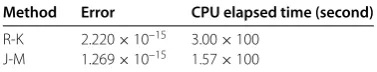
In Figure , we plot the global errorslogofENwith various values ofN. They indicate
that the global errors decay exponentially asN increases. They coincide very well with theoretical analysis.
In Figure , we compare scheme (.) with the four-stage implicit Runge-Kutta method for Example (.) withτ= .,τ= .,τ= .,τ= .,τ= ., in which we takeN= . We find again that the method (.) is more accurate than the corresponding Runge-Kutta methods for largeN.
In Table , we list the numerical errors atx= –. of the four-stage implicit Runge-Kutta withτ= . and the Jacobi spectral method (J-M) for Example (.), and the correspond-ing CPU elapsed time. Clearly, our methods cost nearly the same computational time for obtaining higher numerical accuracy.
In Table , we list the numerical errors atx= . of the four-stage implicit Runge-Kutta withτ= . and the Jacobi spectral method for Example (.), and the corresponding
Figure 4 The absolute error of Example (4.2).
Table 1 Error and CPU elapsed time
Method Error CPU elapsed time (second)
R-K 2.401×10⁻¹⁰ 0.042×100
J-M 1.284×10⁻¹³ 0.30×100
Table 2 Error and CPU elapsed time
Method Error CPU elapsed time (second)
R-K 2.220×10⁻¹⁵ 3.00×100
J-M 1.269×10⁻¹⁵ 1.57×100
CPU elapsed time. Obviously, our methods cost less computational time for obtaining higher numerical accuracy.
5 Concluding remarks
In this paper, we propose a new Jacobi spectral method for the initial problem of first-order ordinary differential equations, which has fascinating advantages.
• The computing scheme is simple and the relevant convergence theory is cleaner and more reasonable than the collocation method.
• The numerical solution is represented by function form, so it can simulate more entirely the global property of exact solution.
• The numerical results demonstrate that the new Jacobi spectral method possesses the spectral accuracy, which coincides with theoretical analysis very well.
• In this paper, we also develop a powerful framework for analyzing various spectral methods of initial value problems of ODEs.
Although we only consider a model problem, the suggested method and technique are also applicable to many other problems, for example infinite-dimensional nonlinear dy-namical system.
Competing interests
The authors declare that they have no competing interests.
Authors’ contributions
Both authors read and approved the final manuscript.
Author details
Acknowledgements
This work was supported in part by the National Natural Science Foundation of China (Grant Nos. 11371074, 11271118, 11301172), the National Natural Science Foundation of China (Tianyuan Fund for Mathematics, Grant No. 11426103), the Natural Science Foundation of Hunan Province (Grant No. 13JJ4095), the Construct Program of the Key Discipline in Hunan Province and the Key Foundation of Hunan Provincial Education Department (Grant No. 11A043).
Received: 30 March 2015 Accepted: 2 July 2015
References
1. Butcher, JC: Implicit Runge-Kutta processes. Math. Comput.18, 50-64 (1964)
2. Butcher, JC: The Numerical Analysis of Ordinary Differential Equations, and General Linear Methods. Wiley, Chichester (1987)
3. Hairer, E, Norsett, SP, Wanner, G: Solving Ordinary Differential Equations I: Nonstiff Problems. Springer, Berlin (1987) 4. Hairer, E, Wanner, G: Solving Ordinary Differential Equations II: Stiff and Differential-Algebraic Problems. Springer,
Berlin (1991)
5. Higham, DJ: Analysis of the Enright-Kamel partitioning method for stiff ordinary differential equations. IMA J. Numer. Anal.9, 1-14 (1989)
6. Stuart, AM, Humphries, AR: Dynamical Systems and Numerical Analysis. Cambridge University Press, Cambridge (1996)
7. Feng, K: Difference schemes for Hamiltonian formalism and symplectic geometry. J. Comput. Math.4, 279-289 (1980) 8. Feng, K, Qin, MZ: Symplectic Geometric Algorithms for Hamiltonian Systems. Zhejiang Science and Technology Press,
Hangzhou (2003)
9. Hairer, E, Lubich, C, Wanner, G: Geometric Numerical Integration: Structure-Preserving Algorithms for Ordinary Differential Equations. Springer Series in Computational Mathematics, vol. 31. Springer, Berlin (2002)
10. Guo, B-Y, Wang, Z-Q: Legendre-Gauss collocation methods for ordinary differential equations. Adv. Comput. Math.30, 249-280 (2009)
11. Yan, J-P, Guo, B-Y: A collocation method for initial value problems of second-order ODEs by using Laguerre functions. Numer. Math., Theory Methods Appl.4(2), 283-295 (2012)
12. Zhang, X-Y, Li, Y: Generalized Laguerre pseudospectral method based Laguerre interpolation. Appl. Math. Comput. 219, 2545-2563 (2012)
13. Wang, Z-Q, Guo, B-Y: Legendre-Gauss-Radau collocation method for solving initial value problems of first order ordinary differential equations. J. Sci. Comput.52, 226-255 (2012)
14. Bergh, J, Löfström, J: Interpolation Spaces: An Introduction. Springer, Berlin (1976)
15. Guo, B-Y, Wang, L-L: Jacobi interpolation approximations and their applications to singular differential equations. Adv. Comput. Math.14(3), 227-276 (2001)
16. Guo, B-Y: Jacobi approximation in certain Hilbert spaces and their applications to singular differential equations. J. Math. Anal. Appl.243, 373-408 (2000)