Polar cap ionosphere and thermosphere during the solar minimum period:
EISCAT Svalbard radar observations and GCM simulations
Hitoshi Fujiwara1,2, Satonori Nozawa3, Sawako Maeda4, Yasunobu Ogawa5, Yasunobu Miyoshi6,
Hidekatsu Jin7, Hiroyuki Shinagawa7, and Kaori Terada1
1Department of Geophysics, Tohoku University, Sendai, Japan 2Faculty of Science and Technology, Seikei University, Japan 3Solar Terrestrial Environment Laboratory, Nagoya University, Nagoya, Japan
4Kyoto Women’s University, Kyoto, Japan 5National Institute of Polar Research, Tokyo, Japan
6Department of Earth and Planetary Sciences, Kyushu University, Fukuoka, Japan 7National Institute of Communication Technology, Tokyo, Japan
(Received June 2, 2010; Revised February 14, 2011; Accepted May 6, 2011; Online published July 27, 2012)
The IPY long-run data were obtained from the European Incoherent Scatter Svalbard radar (ESR) observations during March 2007 and February 2008. Since the solar and geomagnetic activities were quite low during the period, this data set is extremely helpful for describing the basic states (ground states) of the thermosphere and ionosphere in the polar cap region. The monthly-averaged ion temperatures for 12 months show similar local time (or UT) variations to each other. The ion temperatures also show significant seasonal variations. The amplitudes of the local time and seasonal variations observed are much larger than the ones predicted by the IRI-2007 model. In addition, we performed numerical simulations with a general circulation model (GCM), which covers all the atmospheric regions, to investigate variations of the neutrals in the polar thermosphere. The GCM simulations show significant variations of the neutral temperature in the polar region in comparison with the NRLMSISE-00 empirical model. These results indicate that both the ions and neutrals would show larger variations than those described by the empirical models, suggesting significant heat sources in the polar cap region even under solar minimum and geomagnetically quiet conditions.
Key words:Polar cap, ionosphere, thermosphere, EISCAT radar, GCM, simulation, IPY, solar minimum.
1.
Introduction
During the last decade, the variations, dynamical fea-tures, temperature and density structures in the polar cap and/or cusp region of the thermosphere/ionosphere have been clarified from radar and satellite observations (e.g., Innis and Conde, 2001; Maeda et al., 2002; L¨uhr et al., 2004; Liuet al., 2005; Fujiwaraet al., 2007; Clemmonset al., 2008; Maedaet al., 2009, and references therein). In ad-dition to recent works, Moe and Moe (2008) have reviewed historical studies on the high-latitude thermospheric mass density anomaly. Some studies have pointed out that there would be significant thermospheric/ionospheric variations in the polar cap and/or cusp region, although significant en-ergy sources were thought to be located in the region near the auroral oval.
Innis and Conde (2001) showed activities of small-scale gravity waves in the polar cap region at about 300-km al-titude from a statistical analysis of the Dynamics Explorer 2 (DE 2) satellite data; the polar cap was filled with fluc-tuations due to gravity waves, although flucfluc-tuations were very few outside the polar cap. The Challenging
Minisatel-Copyright cThe Society of Geomagnetism and Earth, Planetary and Space Sci-ences (SGEPSS); The Seismological Society of Japan; The Volcanological Society of Japan; The Geodetic Society of Japan; The Japanese Society for Planetary Sci-ences; TERRAPUB.
doi:10.5047/eps.2011.05.023
lite Payload (CHAMP) satellite has observed thermospheric mass density. L¨uhr et al. (2004) found density enhance-ments of almost a factor of two at about 450-km altitude when the satellite passed the cusp region, suggesting at-mospheric up-welling caused by local Joule heating in the cusp region. Liuet al.(2005) showed a large discrepancy between the CHAMP observations and the MSISE-90 em-pirical model (Hedin, 1991) in the cusp region at 400-km altitude.
Studies on temperature and energetics in the polar cap and/or cusp region of the thermosphere/ionosphere, partic-ularly at the F region height, are very few. One impor-tant result was presented by Killeenet al. (1995). They showed thermospheric temperature variations at the F re-gion height in the winter polar cap rere-gion during the so-lar minimum and maximum periods from Fabry-Perot in-terferometer measurements. Maeda et al. (2002, 2009) showed ion temperature variations in the polar cap/cusp re-gion from the European incoherent scatter (EISCAT) Sval-bard radar (ESR) observations. Maedaet al.(2009) found high-temperature regions in the flow channel of the polar cap ion-convection due to frictional heating near the fast ion flow channel. From simultaneous observations with the ESR and CUTLASS Finland radar, Fujiwaraet al.(2007) also obtained a significant thermospheric heating rate in the cusp/polar cap region of the upper thermosphere when
460 H. FUJIWARAet al.: POLAR CAP IONOSPHERE AND THERMOSPHERE DURING A SOLAR MINIMUM PERIOD
pulsed ionospheric flows were observed.
Some interesting features of the thermo-sphere/ionosphere in the polar cap/cusp region have been found as above. However, energy and momentum budgets, or generation mechanisms of disturbances in the polar cap/cusp region, are still unknown because of a lack of comprehensive observations in the region. The ESR has provided valuable data of the ionospheric parameters in the polar cap/cusp region. In particular, the ESR observations during the period of International Polar Year (IPY) enable us to understand the ionosphere in the polar cap/cusp region during the solar minimum and geomagnetically quiet conditions which would produce the basic state of the polar cap ionosphere. In the present study, we show diurnal and seasonal variations of the ion temperature at about 300-km altitude obtained from the ESR observations in the IPY period during March 2007 and February 2008. We also show the neutral temperature variations simulated by a general circulation model (GCM) to discuss the relation between the ion and neutral temperatures in the polar cap region.
2.
ESR Observations during the IPY Period
The ESR, which is located on 78.09◦N, 16.03◦E (75.12◦N, 113.00◦E in geomagnetic coordinates), can ob-serve the polar cap/cusp ionosphere from the E to F re-gions. During the IPY period between March 1, 2007, and February 29, 2008, the ESR provided continuous data of the ionospheric parameters. Since the solar and geomagnetic activities were quite low during this period, this data set is extremely helpful for describing the basic states (ground states) of the thermosphere and ionosphere in the polar cap region. The observing modes include field-aligned profiles from about 100- to 500-km altitude (with the ESR 42-m an-tenna) and 30+hour local area scans (for electric field mea-surements) every two weeks. In the present study, we show the ion temperature data obtained in the field-aligned di-rection at about 300-km altitude every 2 minutes. Detailed information of the EISCAT IPY continuous run is described at the web page http://www.eiscat.se/groups/IPY/.3.
GCM Simulations
In the present study, we also show simulation results by a general circulation model (GCM) which was developed by Miyoshi and Fujiwara (2003) as an extension of the mid-dle atmosphere GCM at Kyushu University (Miyahara et al., 1993; Miyoshi, 1999). The GCM was originally devel-oped as a tropospheric GCM at the Japan Meteorological Agency (Kanamitsuet al., 1983), and developed as a com-munity climate model at the University of Tokyo. The GCM was extended to include the processes of the middle atmo-sphere, and then the thermosphere. The details of the GCM have been described in previous works (e.g., Miyoshi and Fujiwara, 2003, 2006, 2008; Fujiwara and Miyoshi, 2006, 2010 and references therein).
In order to describe the thermospheric neutral tempera-ture during the solar minimum and geomagnetically quiet periods, we assume that the cross polar cap potential drop is 30 kV and theF10.7index is 70×10−22W/m2/Hz. Some of the GCM results obtained under the same conditions have
been already shown in Fujiwara and Miyoshi (2010).
4.
Results
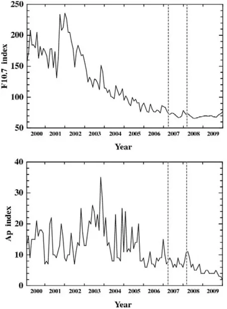
First, we show the monthly-averaged values of theF10.7 and Ap indices from January 2000 to December 2009 in Fig. 1. The vertical dashed lines indicate the period of the IPY observations. Figure 1 shows that the solar radiative flux and geomagnetic activity were quite low during March 2007 and February 2008; the averages of theF10.7and Ap indices during this period are 71.8 and 8, respectively.
The ion temperature in the field-aligned direction at about 300-km altitude is obtained every 2 minutes from the ESR observations. Figure 2 shows examples of the diurnal vari-ations of the ion temperature: the ion temperatures at about 300-km altitude on March 18 and 25, 2007. Although the ESR observations during the IPY period sometimes have data losses, these examples on March 18 and 25 are almost complete data, having only a few data losses during a day. The ion temperature variations in Fig. 2 show spiky excur-sions due to enhancements of the geomagnetic activity, par-ticularly in the case of March 25. In addition, fluctuations with periods from several tens of minutes to 1–2 hours are seen, particularly in the case of March 18. The amplitudes of the fluctuations seem to be several tens to about 100 K.
The ion temperature data at about 300-km altitude ob-tained in the field-aligned direction with the IPY observa-tional mode are divided into 24 UT bins for each month and are averaged; for example, the value plotted at 01:00 UT in Fig. 3 denotes the average of data obtained during 00:30– 01:30 UT. The numbers of the ion temperature data used for the above statistical analysis are 15738 in March 2007, 17443 in April 2007, 14401 in May 2007, 15907 in June 2007, 16939 in July 2007, 12893 in August 2007, 13236 in September, 14306 in October, 3416 in November 2007, 6514 in December 2007, 5436 in January 2008, and 14428 in February 2008. Figure 3 shows UT or local time (the solar local time at the ESR site is UT+1) variations of the averaged ion temperature for 12 months. The numbers la-beled in the figure indicate the month. The ion tempera-tures obtained from the ESR observations show similar UT or local time (LT) variations in all the months. The am-plitudes of the diurnal variations are about 200 K or more. The high temperatures appear at 03:00–05:00 UT (04:00– 06:00 LT) and 11:00–13:00 UT (12:00–14:00 LT). The maximum range of the seasonal variation is about 350 K at around 02:00 UT.
Fig. 1. Monthly-averaged values of theF10.7(upper panel) andAp(bottom
panel) indices from January 2000 to December 2009. The vertical dashed lines indicate the IPY period of the ESR observations.
11:00–12:00 UT.
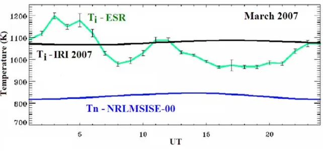
Figure 5 shows the averaged ion temperature obtained from the ESR observations and the ion temperature from the IRI-2007 model in March. The error bars of the ESR ion temperature denote the standard errors of the mean. The IRI temperature is within the range of the ESR temperature vari-ations although the ESR temperature has large amplitudes as mentioned above; the ion temperatures from the ESR ob-servations are about 120 K larger or smaller than those from IRI-2007 in this case. In addition to the ion temperature, the neutral temperature obtained from an empirical model of NRLMSISE-00 (Piconeet al., 2002) is also shown. The ion temperature from IRI-2007 is larger than the neutral tem-perature from NRLMSISE-00 by about 250 K.
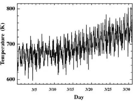
The neutral temperature at about 300-km altitude in March simulated by the GCM is shown in Fig. 6. The GCM data at about 76◦ latitude and 11◦longitude are plotted ev-ery 10 minutes. Figure 6 shows a significant day-to-day variation of the neutral temperature with 2–3 hour fluctu-ations and a seasonal trend. The amplitudes of the neu-tral temperature variations sometimes exceed 100 K in the March case. There are large discrepancies between the val-ues of the neutral temperature from the GCM simulations and NRLMSISE-00, probably because of the ambiguity of NRLMSISE-00 in the polar region and simplified (empiri-cal) high-latitude energy inputs in the present GCM simu-lations.
Fig. 2. Examples of the ion temperature variations at about 300-km alti-tude obtained from the ESR observations. The data of the ion tempera-ture are plotted every 2 minutes. The upper and lower panels show the ion temperature variations on March 18 and 25, respectively.
The neutral temperatures obtained from the GCM sim-ulations are averaged in the same way as the ion temper-atures from the ESR observations shown in Fig. 3. The averaged neutral temperatures are plotted in Fig. 7. The amplitude of the diurnal variation shown in Fig. 7 is 59 K, while that of NRLMSISE-00 is 29 K (see Fig. 5). The maximum temperature is seen at 15:00 UT in Fig. 7, which is similar to NRLMSISE-00 (the maximum temperature of NRLMSISE-00 is at 14:00 UT). The diurnal variation of the GCM temperature shows the second maxima at 01:00 and 22:00 UT, suggesting a relation with the diurnal variation of the ESR ion temperature which also has peaks at 03:00– 05:00 and 22:00–24:00 UT (Fig. 3) or at around 02:00 and 22:00 UT (upper panel of Fig. 2).
5.
Discussion
The solar and geomagnetic activities were quite low dur-ing the IPY ESR observation period (March 2007–February 2008). Small enhancements of the Ap index in Spring and Fall during the IPY period are seen in the lower panel of Fig. 1. This may be a cause of relatively-high ion tempera-tures in March and September in 2007, as shown in Fig. 3.
462 H. FUJIWARAet al.: POLAR CAP IONOSPHERE AND THERMOSPHERE DURING A SOLAR MINIMUM PERIOD
Fig. 3. Monthly-averaged values of the ion temperature obtained from the ESR observations at about 300-km altitude in the field-aligned direction. The numbers labeled in the figure indicate the month.
Fig. 4. Same as Fig. 3 except for the ion temperature obtained from the IRI 2007 model. The ion temperature in each month is shown in the same color as in Fig. 3.
Fig. 5. Monthly-averaged ion temperature obtained from the ESR observations (green line) and the ion temperature from the IRI 2007 model (black line) in March. The error bars of the ESR ion temperature are the standard errors of the mean. In addition to the ion temperature, the neutral temperature obtained from the NRLMSISE-00 model is also shown (blue line).
site even under solar minimum and geomagnetically quiet periods. As shown in Fig. 3, the ion temperature obtained from the ESR observations also show larger amplitudes of diurnal and seasonal variations than those of IRI-2007. The pattern of the diurnal variation of the ion temperature ob-tained from the ESR observations seems to show a better agreement with that of the neutral temperature simulated by the GCM than that of the ion temperature from IRI-2007
and the neutral temperature from NRLMSISE-00 (see up-per panel of Fig. 2 and Fig. 7).
Fig. 6. The neutral temperature at about 300-km altitude at about 76◦ latitude and 11◦longitude in March obtained from the GCM simulation. The GCM data are plotted every 10 minutes.
Fig. 7. Monthly-averaged values of the neutral temperature in March obtained from the GCM simulations at about 300-km altitude. The GCM data are averaged in the same way as the ESR ion temperature shown in Fig. 3.
a day. When heat conduction and energy loss to the elec-trons can be neglected in the steady state, the ion tempera-ture is described as follows (e.g., Schunk and Nagy, 2000),
Ti ≈Tn+
whereTi is the ion temperature (average of perpendicular
and parallel components),Tn is the neutral temperature,kB
is the Boltzmann’s constant, mn is the mean mass of the
neutral gases,Vi is the ion drift velocity,Un is the neutral
wind velocity,Eis the electric field, andBis the geomag-netic field. As shown in Eq. (1), the parameters, Ti, Tn,
Vi (or E), and Un, are related to each other. We should
check the consistency between them, both for specific and statistical (empirical) results. If the difference of 250 K be-tween the ion temperature from IRI-2007 and the neutral temperature from NRLMSISE-00 is correct, a significant electric field would be expected in the polar cap/cusp re-gion even under low solar and geomagnetically quiet peri-ods. From Eq. (1) andTi −Tn = 250 K, we can derive |Vi−Un| ∼589 m/s. When the neutral windUn blows in
the same direction as the ion flow, and the strength of the magnetic field is∼48000 nT, the amplitude of the electric field is estimated as |E| ∼ 28, 33, 38, and 43 mV/m for
Un = 0, 100, 200, and 300 m/s, respectively. This may
underestimate the electric field because of the assumption of the wind direction. The lower limit of the magnitude of the electric field is 28 mV/m, although this value is not so realistic. So, we can make a rough estimate of the electric field as 30∼several 10 mV/m, which would be required to cause the temperature difference (Ti−Tn) of 250 K.
In addition to the in-situ forcing/heating in the polar cap/cusp region of the ionosphere and thermosphere, lower atmospheric effects on the temperature and wind variations would be expected (Fujiwara and Miyoshi, 2009, 2010). Fujiwara and Miyoshi (2010) suggested fluctuations in the polar upper thermosphere with periods of 2–3 hours, due to effects from the lower atmosphere. As seen in Fig. 2, the ion temperature variations also include fluctuations with pe-riods from several tens of minutes to 1–2 hours, suggesting lower atmospheric effects. The amplitudes of the ion tem-perature fluctuations seem to be in agreement with the am-plitudes of the neutral temperature fluctuations (∼several tens of K) simulated by the GCM (Fujiwara and Miyoshi, 2010).
Some researchers have pointed out the importance of the electric field fluctuations for an estimation of the Joule heat-ing rate in the thermosphere (e.g., Codrescuet al., 1995; Matsuoet al., 2003; Matsuo and Richmond, 2008; Deng
et al., 2009). Deng et al. (2009) estimated the altitude-integrated Joule heating, taking into account the electric field variability. They showed large heating rates during about 02:00–13:00 LT at around the 78◦ latitude region when the IMF conditions wereBy = 0 andBz = −5 nT,
the hemispheric power of precipitating auroral particles was 30 GW, and F10.7 was 150×10−22 W/m2/Hz (figure 1 in their paper). They also pointed out that the horizontal dis-tributions of the altitude-integrated Joule heating and the Poynting flux had some detailed differences in the polar cap and nightside regions, when they considered an elec-tric field variability component consistent with the average electric field. The ion temperature with large peaks during 03:00–05:00 UT, seen in all the months (Fig. 3), may be caused by the above heating effects. The monthly-averaged pattern of the high-latitude electric field (or frictional heat-ing) may be almost independent of season in the polar cap region when the geomagnetic activity is not so variable. In addition, if the solar EUV heating is the dominant heat source, the ion temperature should show a dependence on the solar zenith angle. In the cases of other conditions of solar activity, the local time (or UT) variation may be differ-ent for each month; for example, the contributions of solar heating and collisions with neutrals to the energy budget of the polar cap ionosphere may be different from those in the present case. Therefore, the ion temperature variations in the polar cap ionosphere obtained from the IPY data should be important as an experimental proof in the low-solar con-dition.
As mentioned in the previous section, there are large dis-crepancies between the neutral temperatures (Tn) obtained
from the GCM and NRLMSISE-00 (the GCM temperature is about 100 K lower than that from NRLMSISE-00), al-though the pattern of the diurnal variation of Tn, derived
464 H. FUJIWARAet al.: POLAR CAP IONOSPHERE AND THERMOSPHERE DURING A SOLAR MINIMUM PERIOD
with that of the ion temperature (Ti) obtained from the ESR
observations than those ofTi from IRI-2007 andTn from
NRLMSISE-00. The empirical electric field used in the GCM includes a diurnal (or UT) variation which would cause both direct heating in the polar cap region and heat transport from the auroral region to the polar cap (e.g., Fujiwara and Miyoshi, 2010); however, the empirical model does not include localized structures and does not describe localized heating which would be associated with fluctua-tions of the electric field. The electric field, or frictional heating, mentioned above should be one of the most im-portant factors to understand the relations and discrepancies between the temperatures from observations and models in the polar cap region.
Since the ion and neutral temperatures result from the heating and cooling processes, we should clarify the clima-tology of the ion and neutral temperatures in the polar cap ionosphere/thermosphere to understand the energy budget in the region, both from observations and GCM simulations. In the future work, the ion temperatures obtained from the ESR observations will be compared with those simulated by our coupled whole atmosphere-ionosphere GCM, with which preliminary simulations (e.g., Jinet al., 2008, 2011) have been carried out.
6.
Summary
We have investigated the ion temperature variations in the polar cap/cusp region of the thermosphere/ionosphere at about 300-km altitude during the solar minimum and geomagnetically quiet periods. The IPY long-run data, which were obtained from the European Incoherent Scat-ter Svalbard radar (ESR) observations, during March 2007 and February 2008, are extremely helpful for describing the basic states (ground states) of the thermosphere and iono-sphere during the solar minimum and geomagnetically quiet periods in the polar cap region.
The ion temperature obtained from the ESR observa-tions shows spiky excursions due to enhancements of the geomagnetic activity. In addition, fluctuations with peri-ods from several tens of minutes to 1–2 hours are found in the ion temperature variations. The periods and amplitudes (several tens to about 100 K) of the fluctuations seem to be in agreement with those of the neutral temperature varia-tions simulated by the whole atmosphere GCM. This sug-gests that the observed ion temperature variations would in-clude fluctuations due to the lower atmospheric effects with amplitudes of several tens to about 100 K in this case. In ad-dition, the diurnal variation of the ion temperature obtained from the ESR observations is almost in agreement with the diurnal variation of the neutral temperature simulated by the GCM.
The monthly-averaged ion temperatures for 12 months show similar local time (or UT) variations to each other; high temperatures appear at 03:00–05:00 UT (04:00– 06:00 LT), 11:00–13:00 UT (12:00–14:00 LT), and 22:00– 24:00 (23:00–01:00 LT). The ion temperatures also show significant seasonal variations. The amplitudes of the lo-cal time and seasonal variations observed are much larger than the ones predicted by the International Reference Iono-sphere 2007 (IRI-2007) model. The GCM simulations show
significant variations of the neutral temperature in the polar region compared with the NRLMSISE-00 empirical model. These results indicate that both the ions and neutrals would show larger variations than those described by the empirical models.
The ion temperature obtained from IRI-2007 is larger than the neutral temperature from NRLMSISE-00 by about 250 K over the ESR site. Since the ion temperatures ob-tained from the ESR observations vary with large ampli-tudes, the discrepancy between the ion and neutral tempera-tures would be larger than 250 K at a certain moment during a day, suggesting significant heat sources in the polar cap re-gion even under solar minimum and geomagnetically quiet conditions. The ion and neutral temperatures, ion veloc-ity (or electric field), and neutral wind velocveloc-ity are closely related to each other. We should check the consistency be-tween them, both for specific and statistical (empirical) re-sults from comprehensive observations and simulations.
Acknowledgments. We thank the staff of EISCAT for operating the facilities. EISCAT is an international association supported by research organizations in China, Finland, Germany, Japan, Norway, Sweden, and the United Kingdom. This work was sup-ported in part by Grant-in-Aid for Scientific Research C and B (20540435, 23340144, 23340149) and Scientific Research on In-novative Areas (20200047), and the Global COE program “Global Education and Research Center for Earth and Planetary Dynam-ics” at Tohoku University by the Ministry of Education, Science, Sports and Culture, Japan. A part of this work was also supported by the joint research programs of the Solar-Terrestrial Environ-ment Laboratory, Nagoya University and the National Institute of Polar Research, Japan. The empirical models of NRLMSISE-00, IRI 2007, and the solar indices, are provided from NASA/NSSDC, web of NASA/GSFC, and NOAA/NGDC, respectively.
References
Bilitza, D. and B. W. Reinisch, International reference ionosphere 2007: Improvements and new parameters,Adv. Space Res.,42, 599–609, 2008. Clemmons, J. H., J. H. Hecht, D. R. Salem, and D. J. Strickland, Thermo-spheric density in the Earth’s magnetic cusp as observed by the Streak mission,Geophys. Res. Lett.,35, L24103, doi:10.1029/2008GL035972, 2008.
Codrescu, M. V., T. J. Fuller-Rowell, and J. C. Foster, On the importance of E-field variability for Joule heating in the high-latitude thermosphere,
Geophys. Res. Lett.,22, 2393–2396, 1995.
Deng, Y., A. Maute, A. D. Richmond, and R. G. Roble, Impact of electric field variability on Joule heating and thermospheric temperature and density,Geophys. Res. Lett.,36, L08105, doi:10.1029/2008GL036916, 2009.
Fujiwara, H. and Y. Miyoshi, Characteristics of the large-scale traveling atmospheric disturbances during geomagnetically quiet and disturbed periods simulated by a whole atmosphere general circulation model,
Geophys. Res. Lett.,33, L20108, doi:10.1029/2006GL027103, 2006. Fujiwara, H. and Y. Miyoshi, Global structure of large-scale disturbances
in the thermosphere produced by effects from the upper and lower regions: simulations by a whole atmosphere GCM,Earth Planets Space, 61, 463–470, 2009.
Fujiwara, H. and Y. Miyoshi, Morphological features and variations of temperature in the upper thermosphere simulated by a whole atmo-sphere GCM,Ann. Geophys.,25, 427–437, 2010.
Fujiwara, H., R. Kataoka, M. Suzuki, S. Maeda, S. Nozawa, K. Hosokawa, H. Fukunishi, N. Sato, and M. Lester, Electromagnetic energy depo-sition rate in the polar upper thermosphere derived from the EISCAT Svalbard radar and CUTLASS Finland radar observations,Ann. Geo-phys.,25, 2393–2403, 2007.
Hedin, A. E., Extension of the MSIS thermosphere model into the middle and lower atmosphere,J. Geophys. Res.,96, 1159–1172, 1991. Innis, J. L. and M. Conde, Thermospheric vertical wind activity maps
Lett.,28, 3847–3850, 2001.
Jin, H., Y. Miyoshi, H. Fujiwara, and H. Shinagawa, Electrodynamics of the formation of ionospheric wavenumber-four longitudinal structure,J. Geophys. Res.,113, A09307, doi:10.1029/2008JA013301, 2008. Jin, H., Y. Miyoshi, H. Fujiwara, H. Shinagawa, K. Terada, N. Terada , M.
Ishii, Y. Otsuka, and A. Saito, Vertical connection from the tropospheric activities to the ionospheric longitudinal structure simulated by a new Earth’s whole atmosphere-ionosphere coupled model,J. Geophys. Res., 116, A01316, doi:10.1029/2010JA015925, 2011.
Kanamitsu, M., K. Tada, T. Kudo, N. Sato, and S. Isa, Description of the JMA operational spectral model,J. Meteorol. Soc. Jpn.,61, 812–828, 1983.
Killeen, T. L., Y.-I. Won, R. J. Niciejewski, and A. G. Burns, Upper ther-mosphere winds and temperatures in the geomagnetic polar cap: Solar cycle, geomagnetic activity, and interplanetary magnetic field depen-dencies,J. Geophys. Res.,100, 21,327–21,342, 1995.
Liu, H., H. L¨uhr, V. Henize, and W. K¨ohler, Global distribution of the thermospheric total mass density derived from CHAMP,J. Geophys. Res.,110, A04301, doi:10.1029/2004JA010741, 2005.
L¨uhr, H., M. Rother, W. Kohler, P. Ritter, and L. Grunwaldt, Thermo-spheric up-welling in the cusp region: Evidence from CHAMP obser-vations,Geophys. Res. Lett.,31, L06805, doi:10.1029/2003GL019314, 2004.
Maeda, S., S. Nozawa, M. Sugino, H. Fujiwara, and M. Suzuki, Ion and neutral temperature distributions in the E-region observed by the EIS-CAT Tromso and Svalbard radars,Ann. Geophys.,20, 1415–1427, 2002. Maeda, S., Y. Ogawa, K. Hosokawa, S. Nozawa, S. Oyama, T. Tsuda, and A. Brekke, Ion heating in high-speed flow channel within the duskside cell of the polar-cap ion convection under large IMF-By condition,J. Geophys. Res.,114, A11307, doi:10.1029/2009JA014300, 2009. Matsuo, T. and A. D. Richmond, Effects of high-latitude ionospheric
electric field variability on global thermospheric Joule heating and mechanical energy transfer rate, J. Geophys. Res., 113, A07309,
doi:10.1029/2007JA012993, 2008.
Matsuo, T., A. D. Richmond, and K. Hensel, High-latitude ionospheric electric field variability and electric potential derived from DE-2 plasma drift measurements: Dependence on IMF and dipole tilt,J. Geophys. Res.,108, 1005, doi:10.1029/2002JA009429, 2003.
Miyahara, S., Y. Yoshida, and Y. Miyoshi, Dynamic coupling between the lower and upper atmosphere by tides and gravity waves,J. Atmos. Terr. Phys.,55, 1039–1053, 1993.
Miyoshi, Y., Numerical simulation of the 5-day and 16-day waves in the mesopause region,Earth Planets Space,51, 763–772, 1999.
Miyoshi, Y. and H. Fujiwara, Day-to-day variations of migrating diurnal tide simulated by a GCM from the ground surface to the exobase,
Geophys. Res. Lett.,30, 1789, doi:10.1029/2003GL017695, 2003. Miyoshi, Y. and H. Fujiwara, Excitation mechanism of intraseasonal
oscil-lation in the equatorial mesosphere and lower thermosphere,J. Geophys. Res.,111, D14108, doi:10.1029/2005JD006993, 2006.
Miyoshi, Y. and H. Fujiwara, Gravity waves in the thermosphere simulated by a general circulation model, J. Geophys. Res., 113, doi:10.1029/2007JD008874, 2008.
Moe, K. and M. M. Moe, The high-latitude thermospheric mass density anomaly: A historical review and a semi-empirical model,J. Atmos. Sol. Terr. Phys.,70, 794–802, 2008.
Picone, J. M., A. E. Hedin, D. P. Drob, and A. C. Aikin, NRLMSISE-00 empirical model of the atmosphere: Statistical comparisons and scien-tific issues,J. Geophys. Res.,107, 1468, doi:10.1029/2002JA009430, 2002.
Schunk, R. W. and A. F. Nagy,Ionospheres: Physics, Plasma Physics, and Chemistry, 554 pp., Cambridge University Press, Cambridge, 2000.