Turing instability and Hopf bifurcation in a predator–prey model with delay and predator harvesting

(1)

R E S E A R C H

Open Access

Turing instability and Hopf bifurcation in a

predator–prey model with delay and

predator harvesting

Wenjing Gao

1

_{, Yihui Tong}

1

_{, Lihua Zhai}

1

_{, Ruizhi Yang}

1*

_{and Leiyu Tang}

2

*_{Correspondence:}

yangrz@nefu.edu.cn

1_{Department of Mathematics,}

Northeast Forestry University, Harbin, P.R. China

Full list of author information is available at the end of the article

Abstract

In this paper, we study a predator–prey model with delay and harvesting on predator. We give the conditions for stability and Turing instability of coexisting equilibrium by analyzing the eigenvalue spectrum. By using delay as a bifurcation parameter we give conditions for occurrence of Hopf bifurcation. We investigate the property of

bifurcating period solutions by calculating the normal form. We perform some numerical simulations to support our theoretical result. Our results show that diﬀusion and delay are two factors that should be considered in establishing the predator–prey model, since they can induced the Turing instability and spatially bifurcating period solutions.

MSC: 34K18; 35B32

Keywords: Predator–prey; Delay; Harvesting; Hopf bifurcation

1 Introduction

Biological population dynamics is an important research area in biological mathemat-ics. In biology there are various interactions between diﬀerent populations, such as com-petitive relationship, dependency relationship, predation relationship, and so on. Among them, predation relationship is widespread and studied by many scholars [1–3].

Generally, an ordinary diﬀerential equation system describing the prey–predator model is

˙

u(t) =uφ(u) –ϕ(u,v)v,

˙

v(t) =αϕ(u,v)v–θv,

(1.1)

whereu(t) andv(t) stand for the prey and predator densities. Without predator, the growth law of prey is represented by the functionφ(u),ϕ(u,v) is the functional response,αstands for the conversion rate, andθ is the death rate.

The functional response is essential for establishing the predator–prey model. It re-ﬂects the predator’s predation ability and can be aﬀected by many factors, such as structure of the habitat structure, hunting ability, prey’s escape ability, and others. In

(2)

predator–prey models, scholars have used diﬀerent functional responses to model the interaction of predator and prey; they show that the functional response can enrich the model dynamics [4,5]. One kind of commonly used functional response functions are Holling type I–III [6], usually called the prey-dependent functional response (with

ϕ(u,v) denoted asϕ(u), a function of preyu). Another kind of functional response

func-tions are Beddington–DeAngelis type [7], Crowley–Martin type [8], Hassell–Varley type [9], usually called predator-dependent (with ϕ(u,v) a function of prey u and preda-torv).

The Crowley–Martin functional response is of the following form:

g(u,v) = Ev (1 +Su)(1 +Bv),

whereE,S, andBstand for the capture rate of predator to prey, the handling time, and the magnitude of interference among predators, respectively. Cao and Jiang [10] studied a reaction–diﬀusion type predator–prey model with Crowley–Martin functional response, mainly focusing on Turing–Hopf bifurcation. In [11], the authors studied a predator–prey model with delay and Crowley–Martin functional response, mainly considering the sta-bility and Hopf bifurcation. In [12], the authors considered a predator–prey model with Crowley–Martin functional response, mainly studying the ﬂip bifurcation and Neimark– Sacker bifurcation. These works all suggest that the Crowley–Martin functional response can enrich the dynamics of predator–prey models. In this paper, we mainly study a predator–prey model with Crowley–Martin functional response.

To rationally develop the exploitation of biological resources, many scholars have con-sidered predator–prey models with harvesting. The harvesting can be mainly divided into three types: (i) constant harvesting, (ii) proportional harvesting, and (iii) nonlinear-type harvesting (i.e., the harvesting is a nonlinear function). From a biological and economic perspective, more and more scholars recommend Michaelis–Menten type-harvesting [13–16], which has the following form:

h(E,u) = QEu

ηE+βu,

whereQandErepresent the catch ability coeﬃcient and external eﬀort, respectively, and

ηandβare suitable constants. Constant harvesting and proportional harvesting can be

considered as two particular cases of the Michaelis–Menten-type harvesting. In [13], the authors studied the periodic solution of a prey–predator model with harvesting. Yuan et al. [15] studied bifurcation of a delayed predator–prey model with Michaelis–Menten-type prey harvesting. These works suggest that Michaelis–Menten-type harvesting performs well.

(3)

Motivated by these, we studied a diﬀusive delayed predator–prey model with the fol-lowing form:

⎧ ⎪ ⎪ ⎪ ⎪ ⎪ ⎨ ⎪ ⎪ ⎪ ⎪ ⎪ ⎩

∂u(x,t)

∂t =D1 u+ru(1 – u K) –

Euv

(1+Su)(1+Bv), ∂v(x,t)

∂t =D2 v+

CEu(t–τ)v(t–τ)

(1+Su(t–τ))(1+Bv(t–τ))–Dv–

QEv

ηE+βv, x∈Ω,t> 0,

∂u(x,t) ∂ν =

∂v(x,t)

∂ν = 0, x∈∂Ω,t> 0,

u(x,t) =u1(x,t)≥0, v(x,t) =v1(x,t)≥0, x∈Ω,t∈[–τ, 0],

(1.2)

whereu(x,t) andv(x,t) are the prey and predator densities, respectively,D1 andD2are for diffusive coefficients,randKare the growth rate of prey and the carrying capacity,C is the conversion rate of prey, andτ is for the gestation delay of predator. The harvesting term is a Michaelis–Menten-type harvesting on the predator. The main aim of this paper is to study the diffusion-driven Turing instability and delay-induced Hopf bifurcation.

The paper is organized as follows. In Sect.2, we consider the existence of equilibria of the model. In Sect.3, we study the stability of the coexisting equilibrium. In Sect.4, we analyze the property of Hopf bifurcation. In Sect.5, we give some numerical simulations. Finally, we end the paper with a brief conclusion in Sect.6.

2 Equilibrium analysis

For convenience, we perform nondimensionalization of model (1.2). Denotingu˜=u/K, ˜

v=Ev/r, and˜t=tr, system (1.2) becomes (after dropping tildes) ⎧

⎨ ⎩

∂u(x,t)

∂t =d1 u+u[1 –u– v

(1+au)(1+bv)], ∂v(x,t)

∂t =d2 v+

cu(x,t–τ)v(x,t–τ)

(1+au(x,t–τ))(1+bv(x,t–τ))–dv–

v e+qv,

(2.1)

whered1=D1_r ,d2=D2_r ,a=SK,b=Br E,c=

CEK r ,d=

D r,e=

ηr

Q, andq=

βr2

QE2. We assume that

Ω= (0,lπ), wherel> 0. Solving the equation system

⎧ ⎨ ⎩

u(1 –u–₍₁₊_auv₎₍₁₊_bv₎) = 0,

v(₍₁₊_aucu₎₍₁₊_bv₎–d–_e₊1_qv) = 0, (2.2)

we obtain that (0, 0), and (1, 0) are two boundary equilibria, and the coexisting equilibrium (u∗,v∗) satisﬁesv∗=_1–_b(1–₊_bu_(1–∗)(1+_a₎_uau∗)

∗+abu2

∗andh(u∗) = 0, where

h(u) =β5u5+β4u4+β3u3+β2u2+β1u+β0,

β5=a3b3dqu5,

β4= (3 – 2a)a2b3dq,

β3=ab

a2b2dq–c– 3b2dq+ab+bde+dq+ 2bdq– 6b2dq,

β2=b

–cq+b2dq+a2–dq+ 3b2dq–b(1 +de+ 2dq) (2.3)

+a–6b2dq+ (c+ 2d)q+ 2b(1 +de+ 2dq),

β1= –2b3dq+b(c+d)q–c(e+q) +b2

(4)

+a1 +b1 +d(e–q)+ 3b3dq+d(e+q) – 2b21 +d(e+ 2q),

β0=

–1 –b+b2–1 –de+q(1 –b).

We just give a suﬃcient condition for the existence of coexisting equilibrium (u∗,v∗):

a< 1, b< 1, and c> (1 +a)(1 +b)d+ 1/(q+e) . (2.4)

Theorem 2.1 If the parameters satisfy condition(2.4),then model (2.1)has a coexist-ing equilibrium (u∗,v∗), where u∗ is the root of h(u∗) = 0in the region (0, 1), and v∗=

(1–u∗)(1+au∗) 1–b+b(1–a)u∗+abu2∗.

Proof By direct calculation we haveh(0) = (–1 –b+b2_{)(–1 –}_d(e₊_{q(1 –}_{b))) > 0 and}_{h(1) =} (a+ 1)(b+ 1)(1 +d(e+q)) –ce–cq< 0 under condition (2.4). By the continuity ofh(u) we obtain thath(u) = 0 has at least one rootu∗in the (0, 1). Thenv∗=_1–_b(1–₊_bu_(1–∗)(1+_a₎_uau_∗₊∗_abu) 2

∗> 0.

3 Stability analysis

Linearize system (2.1) at (u∗,v∗):

∂u

∂t

∂v

∂t

=diag{d1,d2}

u(t) v(t)

+L1

u(t) v(t)

+L2

u(t–τ) v(t–τ)

, (3.1)

where

L1=

a1 –a2 0 –a3

, L2=

0 0

b1 b2

,

and

a1=u∗

av∗

(1 +au∗)2_{(1 +}_bv_∗₎– 1

, a2=

u∗

(1 +au∗)(1 +bv∗)2 > 0,

a3=d+ e

(e+qv∗)2 > 0, b1=

cv∗

(1 +au∗)2(1 +bv∗)> 0,

b2= cu∗

(1 +au∗)(1 +bv∗)2 > 0.

The characteristic equation is

detλI–Mn–L1–L2e–λτ

= 0, (3.2)

whereI=diag{1, 1}andMn= –n2/l2diag{d1,d2},n∈N0. Then we have

λ2+λAn+Bn+ (Cn–λb2)e–λτ= 0, n∈N0N∪ {0}, (3.3)

where

An= (d1+d2)

n2

(5)

Bn=d1d2

n4

l4 + (a3d1–a1d2) n2

l2 –a1a3,

Cn= –d1b2 n2

l2 +a2b1+a1b2.

3.1 The case

τ

= 0

Whenτ= 0, Eq. (3.3) reduces to the equation

λ2–trnλ+ n= 0, n∈N0, (3.4)

where ⎧ ⎨ ⎩

trn=a1–a3+b2–n 2

l2(d1+d2),

n=a2b1+a1(b2–a3) – [(b2–a3)d1+a1d2]n 2

l2 +d1d2n 4

l4,

(3.5)

and the eigenvalues are given by

λ(_1,2n)=trn±

tr2

n– 4 n

2 , n∈N0. (3.6)

We make the following hypothesis:

(H1) a1–a3+b2< 0, and a2b1+a1(b2–a3) > 0.

Whend1=d2= 0 andτ= 0, (u∗,v∗) is locally asymptotically stable under hypothesis (H1).

Divide the parameters into the following three cases:

Case 1: (b2–a3)d1+a1d2≤0,

Case 2: (b2–a3)d1+a1d2> 0, and

(b2–a3)d1+a1d2 2

– 4d1d2

a2b1+a1(b2–a3)

< 0,

Case 3: (b2–a3)d1+a1d2> 0, and

(b2–a3)d1+a1d22– 4d1d2a2b1+a1(b2–a3)> 0.

(3.7)

Denote

K1{k∈N| k≤0}, K2{k∈N| k< 0},

where kis deﬁned in (3.5).

Theorem 3.1 Suppose(H1)holds andτ= 0.

(1) InCase 1(orCase 2),(u∗,v∗)is locally asymptotically stable;

(2) InCase 3,ifK1=∅,then(u∗,v∗)is locally asymptotically stable;

(3) InCase 3,ifK2=∅,then(u∗,v∗)is Turing unstable.

(6)

negative real parts. This implies that statement (1) holds. Similarly, statement (2) holds. In Case 3, k< 0 fork∈K2. Then Eq. (3.4) has a positive real part root. Then statement

(3) is true.

3.2 The case

τ

= 0

Next, we study the stability of (u∗,v∗) when τ > 0. Letting iω (ω> 0) be a solution of Eq. (3.3), we have

–ω2+iωAn+Bn+ (Cn–iωb2)(cosωτ–isinωτ) = 0.

Then ⎧ ⎨ ⎩

–ω2+Bn+Cncosωτ–ωb2sinωτ= 0,

Anω–Cnsinωτ–ωb2cosωτ= 0,

leading to

ω4+A2_n– 2Bn–b22

ω2+B2_n–C_n2= 0. (3.8)

Denotingz=ω2_{, we can change (3.8) to}

z2+A2_n– 2Bn–b22

z+B2_n–C_n2= 0 = 0, (3.9)

and the roots of (3.9) are

z±=1 2

–A2_n– 2Bn–b22

±A2

n– 2Bn–b22 2

– 4B2

n–C2n

.

Under condition (1) (or 2) of Theorem (3.1), we have

Bn+Cn= n> 0.

Denote

Pn=A2n– 2Bn–b22=

a1–d1 n2

l2 2

+

a3+d2 n2

l2 2

–b2₂,

Qn=Bn–Cn=d1d2

n4

l4 + (b2d1+a3d1–a1d2) n2

l2 – (a1a3+a2b1+a1b2).

Deﬁne

S1={n|Qn< 0,n∈N0},

S2=

n|Qn> 0,Pn< 0,P2n– 4

B2_n–C2_nQn> 0,n∈N0

,

S3=

n|Qn> 0,Pn2– 4

B2_n–C_n2Qn< 0,n∈N0

(7)

and

Lemma 3.1 Assume that(H1)holds and the parameters satisfy the condition(1) (or2)of

Theorem3.1.

Proof Equation (3.9) has a (two or no) positive root(s)z+

n(orz±n) whenn∈S1(n∈S2 or n∈S3). Then statements (1), (2), and (3) are true.

Lemma 3.2 Assume that(H1)holds and the parameters satisfy condition(1) (or2)of

The-orem3.1.ThenRe(d_dλ_τ)|_τ_=τj,+

n > 0andRe( dλ

dτ)|τ=τnj,–< 0for n∈S1∪S2and j∈N0.

Proof Diﬀerentiating Eq. (3.3) with respect toτ, we obtain

S1∪S2}. By the preceding we obtain the following theorem.

Theorem 3.2 Assume that(H1)holds and the parameters satisfy condition(1) (or2)of

Theorem3.1.

(1) (u∗,v∗)is locally asymptotically stable for allτ≥0whenS1∪S2=∅. (2) (u∗,v∗)is locally asymptotically stable forτ∈[0,τ∗)whenS1∪S2=∅. (3) Hopf bifurcation occurs at(u∗,v∗)whenτ=τnj,+(τ=τnj,–),j∈N0,n∈S1∪S2.

4 Property of Hopf bifurcation

(8)

system (2.1) is (dropping the tilde) ⎧

⎨ ⎩

∂u

∂t =τ[d1 u+ (u+u∗)(1 – (u+u∗) –

v+v∗

(1+a(u+u∗))(1+b(v+v∗)))], ∂v

∂t =τ[d2 v+

c(u(t–1)+u∗)(v(t–1)+v∗)

(1+a(u(t–1)+u∗))(1+b(v(t–1)+v∗))–d(v+v∗) –

v+v∗

e+q(v+v∗)].

(4.1)

Denoteτ=τ˜+εandU= (u(x,t),v(x,t))T_{. In the phase space}_C

1:=C([–1, 0],X), (4.1) can be rewritten as

dU(t)

dt =τ˜D U(t) +Lτ˜(Ut) +F(Ut,ε), (4.2)

whereLε(ϕ) andF(ϕ,ε) are

Lε(ϕ) =ε

a1ϕ1(0) –a2ϕ2(0) –a3ϕ2(0) +b1ϕ1(–1) +b2ϕ2(–1)

(4.3)

and

F(ϕ,ε) =εD ϕ+Lε(ϕ) +f(ϕ,ε) (4.4)

with

f(ϕ,ε) = (τ˜+ε)f1(ϕ,ε),f2(ϕ,ε)T,

f1(ϕ,ε) =ϕ1(0) +u∗1 –ϕ1(0) –u∗– ϕ2(0) +v∗

(1 +a(ϕ1(0) +u∗))(1 +b(ϕ2(0) +v∗))

–a1ϕ1(0) +a2ϕ2(0),

f2(ϕ,ε) = (ϕ1(–1) +u∗)(ϕ2(–1) +v∗)

(1 +a(ϕ1(–1) +u∗))(1 +b(ϕ2(–1) +v∗))–d

ϕ2(0) +v∗

– ϕ2(0) +v∗ e+q(ϕ2(0) +v∗)

+a3ϕ2(0) –b1ϕ1(–1) –b2ϕ2(–1)

forϕ= (ϕ1,ϕ2)T_∈_C_1.

We know thatΛn:={iωnτ˜, –iωnτ˜}are characteristic roots of

dz(t) dt = –τ˜D

n2

l2z(t) +Lτ˜(zt). (4.5)

By the Riesz representation theorem there exists a 2×2 matrix functionηn(s,τ˜) (–1≤s≤ 0) with elements of bounded variation functions such that

–τ˜Dn 2

l2ϕ(0) +Lτ˜(ϕ) = 0

–1

dηn(s,τ)ϕ(s)

forϕ∈C([–1, 0],R2). Choose

ηn(s,τ) = ⎧ ⎪ ⎪ ⎨ ⎪ ⎪ ⎩

τE, s= 0,

0, s∈(–1, 0),

–τF, s= –1,

(9)

where

Deﬁne the bilinear paring

(10)

and

u,v := 1 lπ

lπ

0

u1v1dx+ 1 lπ

lπ

0

u2v2dx

foru= (u1,u2),v= (v1,v2),u,v∈X, andϕ,f0 = (ϕ,f1

0 ,ϕ,f02 )T. Rewrite Eq. (4.1) in the abstract form

dU(t)

dt =Aτ˜Ut+R(Ut,ε), (4.9)

where

R(Ut,ε) =

⎧ ⎨ ⎩

0, θ∈[–1, 0),

F(Ut,ε), θ= 0.

(4.10)

The solution is

Ut=Φ

x1 x2

fn+h(x1,x2,ε), (4.11)

where

x1 x2

=Υ,Ut,fn

and

h(x1,x2,ε)∈PSC1, h(0, 0, 0) = 0, Dh(0, 0, 0) = 0.

Then

Ut=Φ

x1(t) x2(t)

fn+h(x1,x2, 0). (4.12)

Letz=x1–ix2and notice thatp1=Φ1+iΦ2. Then

Φ

x1 x2

fn= (Φ1,Φ2)

z+z

2

i(z–z) 2

fn=

1

2(p1z+p1z)fn

and

h(x1,x2, 0) =h

z+z 2 ,

i(z–z) 2 , 0

.

Equation (4.12) becomes

Ut=

1

2(p1z+p1z)fn+h

z+z 2 ,

i(z–z) 2 , 0

=1

(11)

(12)

(13)

χ1=W11(1)(0)(2α1+α2ζ) +W11(2)(0)(α2+ 2α3ζ) From [21] we have

(14)

where

H(z,z) =H20 z2

2 +W11zz+H02 z2

2 +· · ·

=X0F(Ut, 0) –Φ

Υ,X0F(Ut, 0),fn

·fn

. (4.24)

Hence we have

(2iωnτ˜–Aτ˜)W20=H20, –Aτ˜W11=H11, (–2iωnτ˜–Aτ˜)W02=H02, (4.25)

that is,

W20= (2iωnτ˜–Aτ˜)–1H20, W11= –A–1τ˜ H11,

W02= (–2iωnτ˜–Aτ˜)–1H02.

(4.26)

Then

H(z,z) = –Φ(0)Υ(0)F(Ut, 0),fn

·fn

= –

p1(θ) +p2(θ)

2 ,

p1(θ) –p2(θ) 2i

Φ1(0)

Φ2(0)

F(Ut, 0),fn

·fn

= –1 2

p1(θ)Φ1(0) –iΦ2(0)+p2(θ)Φ1(0) +iΦ2(0) F(Ut, 0),fn

·fn

= –1 2

p1(θ)g20+p2(θ)g₀₂z 2

2 +

p1(θ)g11+p2(θ)g₁₁zz

+p1(θ)g02+p2(θ)g₂₀z 2

2

+· · ·.

Therefore

H20(θ) = ⎧ ⎨ ⎩

0, n∈N,

–1₂(p1(θ)g20+p2(θ)g₀₂)·f0, n= 0,

H11(θ) = ⎧ ⎨ ⎩

0, n∈N,

–1₂(p1(θ)g11+p2(θ)g11)·f0, n= 0,

H02(θ) = ⎧ ⎨ ⎩

0, n∈N,

–1₂(p1(θ)g02+p2(θ)g₂₀)·f0, n= 0,

and

H(z,z)(0) =F(Ut, 0) –Φ

Υ,F(Ut, 0),fn

(15)

(16)

where

E=

2iωnτ˜+d1n 2

l2 –a1 a2

–b1e–2iωnτ˜ 2iωnτ˜+d2n

2

l2 +a3–b2e–2iωnτ˜ –1

.

Similarly, from (4.26) we have

–W11˙ = i 2ωnτ˜

p1(θ)g11+p2(θ)g₁₁·fn, –1≤θ< 0,

that is,

W11(θ) = i 2iωnτ˜

p1(θ)g₁₁–p1(θ)g11+E2.

Similarly, we have

E2=τ˜E∗

χ11

ς11

cos2

nx l

,

where

E∗=

d1n_l22 –a1 ra2

–b1 d2n_l22–b2+a3

–1 .

Thus we have:

c1(0) = i 2ωnτ˜

g20g11– 2|g11|2–|g02| 2

3

+1

2g21, μ2= –

Re(c1(0)) Re(λ(τnj))

,

T2= – 1

ωnτ˜

Imc1(0)+ε2Im

λτ_nj , β2= 2Re

c1(0).

(4.28)

Theorem 4.1 For any critical valueτnj,+(orτnj,–),the bifurcating periodic solutions exist

forτ>τnj,±(orτ <τnj,±)whenμ2> 0 (orμ2< 0)and are orbitally asymptotically stable(or unstable)whenβ2< 0 (orβ2> 0).

5 Numerical simulations

To verify our theoretical results, we give some numerical simulations. Fix the following parameters

a= 0.4, b= 0.5, c= 2, d= 0.1, e= 2,

q= 8, d1= 0.1, d2= 0.2, l= 2.

(5.1)

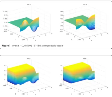
Then (u∗,v∗) = (0.1606, 1.6143) is a unique coexisting equilibrium. Hypothesis (H1) is

sat-isﬁed, and the parameters are in Case 1. By calculation we haveτ∗=τ₀0≈2.3471. By The-orem3.1we have that (u∗,v∗) is stable whenτ ∈[0,τ∗), which is shown in Fig.1;τ =τ∗

is the critical value. Whenτ crosses it, the stability of (u∗,v∗) changes, and bifurcating

solution occurs. By calculation we have

(17)

Figure 1Whenτ= 2, (0.1606, 1.6143) is asymptotically stable

Figure 2Whenτ= 2.5, (0.1606, 1.6143) is is unstable, and stable bifurcating periodic solutions appear

Hence the locally asymptotically stable bifurcating periodic solutions appears for τ > 2.3471, which is shown in Fig.2.

6 Conclusion

We have studied the impact of delay on the dynamics of a diffusive predator–prey model. In this model the functional response is of Crowley–Martin type, and the harvesting of predator is modeled by Michaelis–Menten-type harvesting. We give a sufficient condi-tion (2.4) for coexisting equilibrium to exist. When time delayτ = 0, the stability of coex-isting equilibrium is investigated, and the conditions for stability and Turing instability are given in Theorem3.1. When time delayτincreases, it can affect the stability of coexisting equilibrium and induce Hopf bifurcation. In addition, the property of Hopf bifurcation is considered, including the direction and stability of bifurcating period solutions. Our re-sults suggest that diffusion and time delay are two factors that should be considered in establishing the predator–prey model, since they can induce the Turing instability and spatially bifurcating period solutions.

Acknowledgements

The authors wish to express their gratitude to the editors and the reviewers for the helpful comments.

Funding

(18)

Competing interests

The authors declare that they have no competing interests.

Authors’ contributions

The idea of this research was introduced by WG and RY. All authors contributed to the main results and numerical simulations. All authors read and approved the ﬁnal manuscript.

Author details

1_{Department of Mathematics, Northeast Forestry University, Harbin, P.R. China.}2_{College of Mathematics and Systems}

Science, Shandong University of Science and Technology, Qingdao, P.R. China.

Publisher’s Note

Springer Nature remains neutral with regard to jurisdictional claims in published maps and institutional aﬃliations.

Received: 17 April 2019 Accepted: 20 June 2019 References

1. Yi, F., Wei, J., Shi, J.: Bifurcation and spatiotemporal patterns in a homogeneous diﬀusive predator–prey system. J. Diﬀer. Equ.246(5), 1944–1977 (2009)

2. Zhang, T., Meng, X., Song, Y., et al.: A stage-structured predator–prey SI model with disease in the prey and impulsive eﬀects. Math. Model. Anal.18(4), 505–528 (2013)

3. Wang, J., Shi, J., Wei, J.: Dynamics and pattern formation in a diffusive predator–prey system with strong Allee effect in prey. J. Differ. Equ.251, 1276–1304 (2011)

4. Jana, D., Pathak, R., Agarwal, M.: On the stability and Hopf bifurcation of a prey–generalist predator system with independent age-selective harvesting. Chaos Solitons Fractals83(83), 252–273 (2016)

5. Yuan, R., Jiang, W., Wang, Y.: Saddle-node-Hopf bifurcation in a modiﬁed Leslie–Gower predator–prey model with time-delay and prey harvesting. J. Math. Anal. Appl.422(2), 1072–1090 (2015)

6. Holling, C.S.: The functional response of predators to prey density and its role in mimicry and population regulation. Mem. Entomol. Soc. Can.97(45), 1–60 (1965)

7. Beddington, J.R.: Mutual interference between parasites or predators and its eﬀect on searching eﬃciency. J. Anim. Ecol.44(1), 331–340 (1975)

8. Crowley, P.H., Martin, E.K.: Functional responses and interference within and between year classes of a dragonﬂy population. J. North Am. Benthol. Soc.8(3), 211–221 (1989)

9. Hassell, M.P., Varley, G.C.: New inductive population model for insect parasites and its bearing on biological control. Nature223(5211), 1133–1137 (1969)

10. Cao, X., Jiang, W.: Turing–Hopf bifurcation and spatiotemporal patterns in a diﬀusive predator–prey system with Crowley–Martin functional response. Nonlinear Anal., Real World Appl.43, 428–450 (2018)

11. Tripathi, J.P., Tyagi, S., Abbas, S.: Global analysis of a delayed density dependent predator–prey model with Crowley–Martin functional response. Commun. Nonlinear Sci. Numer. Simul.30(1–3), 45–69 (2016)

12. Ren, J., Yu, L., Siegmund, S.: Bifurcations and chaos in a discrete predator–prey model with Crowley–Martin functional response. Nonlinear Dyn.90, 19–41 (2017)

13. Wang, J., Cheng, H., Liu, H., et al.: Periodic solution and control optimization of a prey–predator model with two types of harvesting. Adv. Diﬀer. Equ.2018(1), 41 (2018)

14. Krishna, S.V., Srinivasu, P.D.N., Kaymakcalan, B.: Conservation of an ecosystem through optimal taxation. Bull. Math. Biol.60(3), 569–584 (1998)

15. Yuan, R., Jiang, W., Wang, Y.: Saddle-node-Hopf bifurcation in a modiﬁed Leslie–Gower predator–prey model with time-delay and prey harvesting. J. Math. Anal. Appl.422(2), 1072–1090 (2015)

16. Clark, C.W.: Mathematical models in the economics of renewable resources. SIAM Rev.21(1), 81–99 (2006) 17. Jiang, Z., Global, W.L.: Hopf bifurcation for a predator–prey system with three delays. Int. J. Bifurc. Chaos27(7),

1750108 (2017)

18. Wang, Z., Wang, X., Li, Y., et al.: Stability and Hopf bifurcation of fractional-order complex-valued single neuron model with time delay. Int. J. Bifurc. Chaos27(13), 1750209 (2017)

19. Liu, G., Wang, X., Men, X., et al.: Extinction and persistence in mean of a novel delay impulsive stochastic infected predator–prey system with jumps. Complexity2017(3), 1–15 (2017)

20. Li, L., Wang, Z., Li, Y., et al.: Hopf bifurcation analysis of a complex-valued neural network model with discrete and distributed delays. Appl. Math. Comput.330, 152–169 (2018)

21. Wu, J.: Theory and Applications of Partial Functional Diﬀerential Equations. Springer, Berlin (1996)