Compact difference scheme for two dimensional fourth order hyperbolic equation

(1)

R E S E A R C H

Open Access

Compact difference scheme for

two-dimensional fourth-order hyperbolic

equation

Qing Li

1

_{and Qing Yang}

1*

*_{Correspondence:}

[email protected]

1_{School of Mathematics and} Statistics, Shandong Normal University, Jinan, China

Abstract

In this paper, we mainly study an initial and boundary value problem of a

two-dimensional fourth-order hyperbolic equation. Firstly, the fourth-order equation is written as a system of two second-order equations by introducing two new variables. Next, in order to design an implicit compact finite difference scheme for the problem, we apply the compact finite difference operators to obtain a fourth-order discretization for the second-order spatial derivatives and the Crank–Nicolson difference scheme to obtain a second-order discretization for the first-order time derivative. We prove the unconditional stability of the scheme by the Fourier method. Then a convergence analysis is given by the energy method. Numerical results are provided to verify the accuracy and efficiency of this scheme.

Keywords: Fourth-order hyperbolic equation; High accuracy method; Compact

diﬀerence scheme; Stability analysis; Convergence analysis

1 Introduction

LetΩ= (0,a)×(0,b) and we consider the two-dimensional fourth-order hyperbolic equa-tion with initial and boundary condiequa-tions:

⎧ ⎪ ⎪ ⎪ ⎪ ⎪ ⎪ ⎪ ⎪ ⎪ ⎪ ⎪ ⎨ ⎪ ⎪ ⎪ ⎪ ⎪ ⎪ ⎪ ⎪ ⎪ ⎪ ⎪ ⎩

(a) utt+ρ2u=f(x,y,t), (x,y,t)∈Ω×(0,T],

(b) u(x,y, 0) =f1(x,y), ∂u_∂t|(x,y,0)=f2(x,y), (x,y)∈Ω,

(c) u|x=0=h1(y,t), u|x=a=h2(y,t),

u|y=0=h3(x,t), u|y=b=h4(x,t), t∈[0,T],

(d) u|x=0=g1(y,t), u|x=a=g2(y,t),

u|y=0=g3(x,t), u|y=b=g4(x,t), t∈[0,T],

(1)

whereutt=∂

2_u

∂t2,2u=

∂4u ∂x4 + 2

∂4u ∂x2_∂y2 +

∂4u

∂y4.f(x,y,t) is the given source term.f1(x,y) and

f2(x,y) are initial value functions.h1(y,t),h2(y,t),h3(x,t),h4(x,t) andg1(y,t),g2(y,t),g3(x,t),

g4(x,t) are boundary value functions.ρis a given positive constant.

The two-dimensional fourth-order hyperbolic equations have very important physical background and a wide range of applications. For example, they can be used to describe the vibration of a plate and in large-scale civil engineering, spaceﬂight, and active noise control

(2)

(see [1–5]). Compared with the second-order equations [6–11], it is usually necessary to use higher-order finite element methods or thirteen-point difference schemes in order to solve the numerical solution of the two-dimensional fourth-order equations. The former is difficult to calculate. The latter has some difficulties to deal with the boundary and only achieves second-order accuracy.

The compact finite difference method, compared to the traditional finite difference method, has a narrower band width and achieves a higher accuracy. Hence, they have long been studied, for example, in [12,13]. In the last few years, high-order computational methods for different kinds of differential equations were studied (see [6–8,12–17]). In [14–16] fourth-order equations are written as a system of two second-order equations by introducing two new variables. Then, in order to design a high-order scheme for the problem, the spatial derivatives are discretized by applying the compact finite difference method or compact volume method.

In this paper, we apply similar ideas to the two-dimensional fourth-order hyperbolic equation (1). Firstly, the fourth-order equation is written as a system of two second-order equations by introducing two new variables. Next, we use the compact operators to ap-proximate the second-order derivatives in the space variables and rewrite the above prob-lem as an initial value probprob-lem for a system of two second-order ordinary differential equa-tions. Then we develop a two time level compact finite difference scheme. We prove the stability for the high-order compact difference scheme by the Fourier method. The con-vergence of the high-order compact difference scheme is given by the energy method.

The rest of the paper is arranged as follows. In Sect.2we formulate the fourth-order compact ﬁnite diﬀerence scheme for problem (1). A stability analysis is given by the Fourier method in Sect.3, and a convergence analysis is given by the energy method in Sect.4.

Numerical experiments are performed in Sect.5to test the accuracy and eﬃciency of the

proposed compact ﬁnite diﬀerence scheme. Conclusions are given in Sect.6.

2 Compact ﬁnite difference scheme

To design a proper ﬁnite diﬀerence scheme, we setv= –ρu, w=∂u_∂t and reformulate

problem (1) in terms of the coupled system of second-order equations

⎧ ⎪ ⎪ ⎪ ⎪ ⎪ ⎪ ⎪ ⎪ ⎪ ⎪ ⎪ ⎪ ⎪ ⎪ ⎨ ⎪ ⎪ ⎪ ⎪ ⎪ ⎪ ⎪ ⎪ ⎪ ⎪ ⎪ ⎪ ⎪ ⎪ ⎩

(a) ∂w_∂t –v=f(x,y,t), (x,y,t)∈Ω×(0,T],

(b) ρw+∂v

∂t = 0, (x,y,t)∈Ω×(0,T],

(c) w(x,y, 0) =f2(x,y), v(x,y, 0) = –ρf1(x,y), (x,y)∈Ω,

(d) w|x=0=∂h1

∂t (y,t), w|x=a= ∂h2

∂t (y,t),

w|y=0=∂h3

∂t (x,t), w|y=b= ∂h4

∂t (x,t), t∈[0,T],

(e) v|x=0= –ρg1(y,t), v|x=a= –ρg2(y,t),

v|y=0= –ρg3(x,t), v|y=b= –ρg4(x,t), t∈[0,T].

(2)

Obviously,uis a solution to (1), if and only if (v,w) is a solution to (2).

Lethx=_N_xa₊₁,hy=_N_yb₊₁ be the spatial step in thexandydirections,τ=T_N be the time

step andxi=ihx, 0≤i≤Nx+ 1,yj=jhy, 0≤j≤Ny+ 1,tk=kτ, 0≤k≤N,h=max{hx,hy}.

The theoretical solutionsu,v,wat the point (xi,yj,tk) are denoted byukij,vkij,wkijand the

(3)

Our compact method for (1) is based on the system (2). To do this, we set

Deﬁning the diﬀerence operators

Ax= 1 +

and applying a Taylor expansion, we get

δ_x2vk_ij= Axθijk+ (Rx)kij, δy2vkij= Ayϑijk+ (Ry)kij,

(4)

where

Replacingvk_i,j,wk_i,jby their approximationsV_i,jk,W_i,jkand neglecting the higher-order terms, we derive a ﬁnite diﬀerence scheme as follows:

⎧

where the discretized boundary values and initial values are denoted by

W_0,jk =∂h1

Remark2.1 From (5) it is easy to see that the local truncation error for this scheme is O(τ2+h4_).

3 Stability analysis

In this section, we adopt the Fourier method to analyze stability of the scheme (6). Assume thath=g(τ), whereg(τ) is a continuous function andg(0) = 0. In order to prove stability of the scheme (6), we consider a diﬀerence scheme of the form

(5)

whereAmandBmare 2×2 matrices,N0andN1are ﬁnite sets containing 0, positive

in-tegers and negative inin-tegers, Um

j is a two-dimensional column vector. Using the Fourier

method we get the growth factorG(xi,yj). Then the scheme (7) is stable if and only if the

family of matrices

Gn(xi,yj);x0= 0 <x1<· · ·<xNx+1=a,

y0= 0 <y1<· · ·<yNy+1=b,n= 1, 2, . . . ,N

(8)

is uniformly bounded. We introduce the following two lemmas.

Lemma 3.1([18]) To prove that the family of matrices(8)is uniformly bounded,it is nec-essary and suﬃcient to prove that the family of matrices

Gn(x,y); 0 <x<a, 0 <y<b,n= 1, 2, . . . (9)

is uniformly bounded.

Proof Accuracy is obvious, we now prove the necessity. We use the meshes withNx= 2m,

Ny= 2k,m= 1, 2, . . . ,k= 1, 2, . . . . Denote by (xp,yq) the grid points in the mesh for given

m and k, wherexp=₂ap,yq=₂bq,p= 1, 2, . . . ,m,q= 1, 2, . . . ,k. Assume

Gn(xp,yq)≤M, 0≤nτ ≤T,

where Mis a constant that has nothing to do with partition. We setτ →0, therefore,

h→0, then

Gn(xp,yq)≤M, n= 1, 2, . . . .

Noting that the bisecting points{(xp,yq)}are dense on [0,a]×[0,b], andG(x,y) is a

con-tinuous function, we get

_Gn₍_x_,_y₎_≤_M_, ₀_≤_x_≤_a_{, 0}_≤_y_≤_b_,_n_{= 1, 2, . . . .}

Lemma 3.2([18]) Assume G(x,y)is an2×2matrices and use gijto represent the element

of the ith row and the jth column.The eigenvalues of G areλ1andλ2.The family of matrices {Gn(x,y)}is uniformly bounded if and only if

⎧ ⎪ ⎪ ⎨ ⎪ ⎪ ⎩

(α) |λi(x,y)| ≤1, i= 1, 2, 0≤x≤a, 0≤y≤b,

(β) G(x,y) –1

2(g11(x,y) +g22(x,y))I

≤M(|1 –|λ1(x,y)||+|λ1(x,y) –λ2(x,y)|), 0≤x≤a, 0≤y≤b.

(10)

Remark3.1

(1) From the relationship between roots and coeﬃcients in the quadric equation λ2–bλ–c= 0, the modulo of two roots is not bigger than one if and only if

(6)

(2) In the condition(β),we need to calculate the norm of a2×2matrix. We usually use theFrobenius-norm, which is deﬁned as

KF=

₂

i,j=1 |kij|2

1 2

, (12)

for a matrixK= (kij).

Theorem 3.1 The scheme(6)is unconditionally stable.

Proof We use the Fourier method to prove the stability of the scheme (6). Using the deﬁ-nitions ofAhandBh, the scheme (6) is written as

⎧ ⎪ ⎪ ⎪ ⎪ ⎪ ⎨ ⎪ ⎪ ⎪ ⎪ ⎪ ⎩

(1) ₁₄₄1 [c1+ 10(c2+c3) + 100c4] –₂₄1(r1d1+ 2r2d2+ 2r3d3– 20r1d4)

=₁₄₄1 [c1+ 10(c2+c3) + 100c4] +₂₄1(r1d1+ 2r2d2+ 2r3d3– 20r1d4),

(2) ₂₄ρ(r1c1+ 2r2c2+ 2r3c3– 20r1c4) +₁₄₄1 [d1+ 10(d2+d3) + 100d4]

=–ρ₂₄(r1c1+ 2r2c2+ 2r3c3– 20r1c4) +₁₄₄1 [d1+ 10(d2+d3) + 100d4],

(13)

where

rx= τ

h2 x

, ry=

τ

h2 y

, r1=rx+ry, r2= 5rx–ry, r3= 5ry–rx,

c1=Wi–1,j–1k+1 +Wi–1,j+1k+1 +Wi+1,j–1k+1 +Wi+1,j+1k+1 ,

c2=Wi–1,jk+1+Wi+1,jk+1, c3=Wi,j–1k+1+Wi,j+1k+1, c4=Wi,jk+1,

d1=Vi–1,j–1k+1 +Vi–1,j+1k+1 +Vi+1,j–1k+1 +Vi+1,j+1k+1 ,

d2=Vi–1,jk+1+Vi+1,jk+1, d3=Vi,j–1k+1+Vi,j+1k+1, d4=Vi,jk+1,

c1=Wi–1,j–1k +Wi–1,j+1k +Wi+1,j–1k +Wi+1,j+1k ,

c2=Wi–1,jk +Wi+1,jk , c3=Wi,j–1k +Wi,j+1k , c4=Wi,jk,

d1=Vi–1,j–1k +Vi–1,j+1k +Vi+1,j–1k +Vi+1,j+1k ,

d2=Vi–1,jk +Vi+1,jk , d3=Vi,j–1k +Vi,j+1k , d4=Vi,jk.

LetWk

jm=vk1eiσ1jhxeiσ2mhy,Vjmk =vk2eiσ1jhxeiσ2mhy, wherevk1andvk2are the amplitude at time

levelk,σ1andσ2represent the wave numbers in thexandydirections. By inserting these

expressions into the coupled scheme (13), we have

1 144

eiσ1(j–1)hx_eiσ2(m–1)hy₊_eiσ1(j–1)hx_eiσ2(m+1)hy₊_eiσ1(j+1)hx_eiσ2(m–1)hy

+eiσ1(j+1)hx_eiσ2(m+1)hy₊ 10

144

eiσ1jhx_eiσ2(m–1)hy₊_eiσ1jhx_eiσ2(m+1)hy

+eiσ1(j–1)hx_eiσ2mhy₊_eiσ1(j+1)hx_eiσ2mhy₊100

144e

iσ1jhx_eiσ2mhy

vk+1₁

–

1

24(rx+ry)

(7)

(8)

(9)

Equations (14) and (15) can be written as

Then from (16) we immediately get the matrix of growth of the scheme (13),

G(σ1hx,σ2hy) =

(10)

Next, we have

Hence, there exists a constantM≥1₂

√ 1+ρ2

√_ρ such that (10β) holds for anyrx> 0,ry> 0.

Then from Lemma3.2we know that the diﬀerence scheme (13) is stable.

4 Error analysis

In this section we give the convergence analysis by the energy method. We introduce the spacesSh={u|u∈R(Nx+2)×(Ny+2)},S0h={u|u∈R(Nx+2)×(Ny+2),u0,j=uNx+1,j=ui,0=uNy+1,0=

For the error analysis, we ﬁrst note that our numerical scheme is based on (5) with

(11)

ρ

2Bh

wk+1_ij +wk_ij+ Ah _vk+1

ij –vkij τ

=gk+ 1 2

ij ,

1≤i≤Nx, 1≤j≤Ny, 1≤k≤N,

where

_gk+1₂_≤

C1

τ2+h4, gk+12≤_C

2

τ2+h4, (23)

withC1,C2positive constants. And our numerical scheme (6) is equivalent to

Ah _Wk+1

ij –Wijk τ

–1

2Bh

V_ijk+1+V_ijk= Ahf k+1₂ ij ,

1≤i≤Nx, 1≤j≤Ny, 1≤k≤N,

ρ

2Bh

W_ijk+1+W_ijk+ Ah _Vk+1

ij –Vijk τ

= 0,

1≤i≤Nx, 1≤j≤Ny, 1≤k≤N.

Lettingξ_i,jk =wk_i,j–W_i,jk andηk_i,j=vk_i,j–V_i,jk replace the approximation errors, we can get the error equations

A_hξ_ijk+1–ξ_ijk–τ 2Bh

ηk+1_ij +η_ijk=τgk+ 1 2

ij ,

1≤i≤Nx, 1≤j≤Ny, 1≤k≤N, (24)

ρτ

2 Bh

ξ_ijk+1+ξ_ijk+ Ah

η_ijk+1–ηk_ij=τgk+ 1 2

ij ,

1≤i≤Nx, 1≤j≤Ny, 1≤k≤N. (25)

Using the discrete Green formula, we know that the difference operatorsδ_x2andδ2_yare self-adjoint and symmetric positive definite. We find that the difference operators Ah, Bh

are self-adjoint and symmetric positive deﬁnite as well. To give the error estimate, the lemmas used later are ﬁrst given as follows.

Lemma 4.1([7]) For any grid function u,v∈S0

h,we have (1) (Ahu,v) = (u, Ahv),(Bhu,v) = (u, Bhv),

(2) (δ2

xu,v) = (u,δ2xv),(δy2u,v) = (u,δy2v).

Lemma 4.2([19,20]) For any grid function u∈S0_h,we have

(1) 2 3u

2_≤_(A

xu,u)≤ u2, 2₃u2≤(Ayu,u)≤ u2; (2) 4₉u2_≤_(A

hu,u)≤ u2; (3) h2

x(Ayδxu,δxu)≤4(Ayu,u),h2y(Axδyu,δyu)≤4(Axu,u).

Theorem 4.1 Let{wk,vk}be the solution of Eq. (2)and{Wk,Vk}be the solution of scheme (6).For the compact ﬁnite diﬀerence scheme,assuming that both rxand ryare bounded,we

have

max

0≤kτ≤T

(12)

Proof Taking the inner product withξk+1₊_ξk_{on both sides of (}₂₄_{), we have}

Ah

ξk+1–ξk,ξk+1+ξk–τ 2

Bh

ηk+1+ηk,ξk+1+ξk=τgk+12_,_ξk+1₊_ξk_. ₍₂₇₎

Taking the inner product withηk+1₊_ηk_{on both sides of (}₂₅_{), we have} ρτ

2

Bh

ξk+1+ξk,ηk+1+ηk+Ah

ηk+1–ηk,ηk+1+ηk=τgk+12_,_ηk+1₊_ηk_. ₍₂₈₎

From Lemma4.1we have

Bh

ηk+1+ηk,ξk+1+ξk=Bh

ξk+1+ξk,ηk+1+ηk. (29)

Multiplying byρboth sides of (27), we have

ρAh

ξk+1–ξk,ξk+1+ξk–ρτ 2

Bh

ηk+1+ηk,ξk+1+ξk

=ρτgk+12_,_ξk+1₊_ξk_. ₍₃₀₎

Combining (28) with (30), we obtain

ρAh

ξk+1–ξk,ξk+1+ξk+Ah

ηk+1–ηk,ηk+1+ηk

=ρτgk+12_,_ξk+1₊_ξk₊_τ_gk+12_,_ηk+1₊_ηk_.

Using Lemma4.1, we obtain

ρAhξk+1,ξk+1

–ρAhξk,ξk

+Ahηk+1,ηk+1

–Ahηk,ηk

=ρτgk+12_,_ξk+1₊_ξk₊_τ_gk+12_,_ηk+1₊_ηk_.

By the inequalityab≤1₂(a2₊_b2_{) and (}_a₊_b₎2_≤₂₍_a2₊_b2_{), we get}

ρAhξk+1,ξk+1

–ρAhξk,ξk

+Ahηk+1,ηk+1

–Ahηk,ηk

≤ρτ

2 g

k+1₂2

+ρτξk+12+ξk2+τ 2g

k+1₂2

+τηk+12+ηk2.

Summingkfrom 0 ton, then

ρAhξn+1,ξn+1

–ρAhξ0,ξ0

+Ahηn+1,ηn+1

–Ahη0,η0

≤τ

2

n

k=0

ρgk+122₊_gk+122₊_ρτ

n

k=0

ξk+12+ξk2

+τ n

k=0

(13)

which implies that

Applying the discrete Gronwall lemma to (32), we get

ρξn+12+ηn+12≤Cτ

This completes the proof.

5 Numerical experiments

In this section we give some numerical results for the two-dimensional model problems given below. These results are obtained by using Matlab.

Example1 We seek the numerical solution for the following problem:

(14)

The theoretical solution is taken as u(x,y,t) =e–πt_sin₍_π_x₎_sin₍_π_y_). _f₍_x_,_y_,_t_{), the initial}

and boundary value functions in (36), can be obtained fromu(x,y,t). We havev(x,y,t) = 2π2e–πtsin(πx)sin(πy) and w(x,y,t) = –πe–πtsin(πx)sin(πy). The compact diﬀerence scheme (6) is used to solve the problem (36). As comparison with our method, the central diﬀerence scheme is used to solve this problem.

In our numerical results, errors and computational orders inL2-norm andL∞-norm of the compact difference scheme and the central difference scheme are given in Tables1–4. From these tables we can find that the compact difference scheme can achieve a higher accuracy and efficiency than the central difference scheme in identical mesh. The exact

Table 1 Errors and computational orders of compact diﬀerence scheme forW

h τ W–wL∞ order≈ W–wL2 order≈ CPU (s)

1 10

1

102 2.408e–03 – 1.204e–03 – 0.210328

1 20

1

202 1.215e–04 4.31 6.076e–05 4.31 2.012129

1 30

1

302 2.192e–05 4.22 1.096e–05 4.22 16.707314

1 40

1

402 6.618e–06 4.16 3.309e–06 4.16 65.458675

1 50

1

502 2.634e–06 4.13 1.317e–06 4.13 192.643835

1 60

1

602 1.246e–06 4.11 6.230e–07 4.11 484.401023

Table 2 Errors and computational orders of central diﬀerence scheme forW

1 10

1

102 1.279e–01 – 6.395e–02 – 0.187456

1 20

1

202 3.655e–02 1.81 1.827e–02 1.81 1.381777

1 30

1

302 1.646e–02 1.97 8.229e–03 1.97 12.942769

1 40

1

402 9.296e–03 1.99 4.648e–03 1.99 53.898653

1 50

1

502 5.960e–03 1.99 2.980e–03 1.99 161.459585

1 60

1

602 4.143e–03 1.99 2.071e–03 1.99 429.255721

Table 3 Errors and computational orders of compact diﬀerence scheme forV

h τ V–vL∞ order≈ V–vL2 order≈ CPU (s)

1 10

1

102 1.306e–03 – 6.532e–04 – 0.210328

1 20

1

202 5.261e–05 4.63 2.631e–05 4.63 2.012129

1 30

1

302 9.433e–06 4.24 4.717e–06 4.24 16.707314

1 40

1

402 2.850e–06 4.16 1.425e–06 4.16 65.458675

1 50

1

502 1.136e–06 4.12 5.680e–07 4.12 192.643835

1 60

1

602 5.379e–07 4.10 2.690e–07 4.10 484.401023

Table 4 Errors and computational orders of central diﬀerence scheme forV

1 10

1

102 8.573e–02 – 4.286e–02 – 0.187456

1 20

1

202 1.447e–02 2.57 7.237e–03 2.57 1.381777

1 30

1

302 6.001e–03 2.17 3.006e–03 2.17 12.942769

1 40

1

402 3.304e–03 2.08 1.652e–03 2.08 53.898653

1 50

1

502 2.092e–03 2.05 1.046e–03 2.05 161.459585

1 60

1

(15)

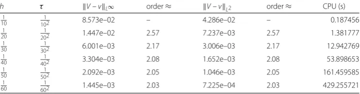
Figure 1Exact solutionv

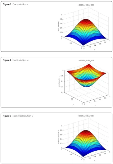
Figure 2Exact solutionw

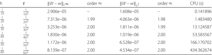
Figure 3Numerical solutionV

results v(x,y,t) andw(x,y,t), with a mesh forhx=hy= 0.05 are plotted in Figs.1and2

fort= 1, respectively. The numerical results{V_ijn+1}and{W_ijn+1}, with a mesh forhx=hy=

0.05, are plotted in Figs.3and4fort= 1.

Example2 We consider the numerical solution for the problem (36) with the exact solu-tion

u(x,y,t) =t2e

–(x–0.5)2–(y–0.5)2

(16)

Figure 4Numerical solutionW

Table 5 Errors and computational orders of compact diﬀerence scheme withβ= 10 forW

1 10

1

102 5.803e–07 – 3.316e–07 – 0.315426

1 20

1

202 4.149e–08 3.81 1.840e–08 4.17 2.235077

1 30

1

302 7.796e–09 4.12 3.417e–09 4.15 16.917521

1 40

1

402 2.358e–09 4.16 1.046e–09 4.11 64.900482

1 50

1

502 9.320e–10 4.16 4.199e–10 4.10 193.079116

1 60

1

602 4.528e–10 3.96 1.998e–10 4.07 494.024067

Table 6 Errors and computational orders of central diﬀerence scheme withβ= 10 forW

1 10

1

102 2.906e–05 – 1.608e–05 – 0.141896

1 20

1

202 7.313e–06 1.99 4.063e–06 1.98 1.483480

1 30

1

302 3.253e–06 2.00 1.811e–06 1.99 13.124587

1 40

1

402 1.830e–06 2.00 1.019e–06 2.00 53.583567

1 50

1

502 1.172e–06 2.00 6.528e–07 2.00 166.170702

1 60

1

602 8.139e–07 2.00 4.534e–07 2.00 434.362674

Then f(x,y,t), the initial and boundary value functions in (36), can be obtained from u(x,y,t). And we get the functions

v(x,y,t) =

4

β –

(2x– 1)2

β2 –

(2y– 1)2

β2

t2e

–(x–0.5)2–(y–0.5)2

β _, ₀≤_x_,_y≤_{1, 0}≤_t≤_1,

w(x,y,t) = 2te

–(x–0.5)2–(y–0.5)2

β _, ₀≤_x_,_y≤_{1, 0}≤_t≤_1.

The compact diﬀerence scheme (6) is used to solve the non-homogeneous problem with

β= 10 andβ=₁₀1.

Errors and computational orders inL2_{-norm and}_L∞_{-norm of the compact diﬀerence}

scheme and the central diﬀerence scheme withβ= 10 are given in Tables5–8. Tables9–12

show errors and computational orders inL2_{-norm and}_L∞_{-norm of the compact}

differ-ence scheme and the central differdiffer-ence scheme withβ= 1

10. From these tables we can see

(17)

diﬀer-Table 7 Errors and computational orders of compact diﬀerence scheme withβ= 10 forV

1 10

1

102 2.711e–07 – 1.367e–07 – 0.315426

1 20

1

202 1.347e–08 4.33 9.382e–09 3.87 2.235077

1 30

1

302 2.201e–09 4.47 1.691e–09 4.23 16.917521

1 40

1

402 6.851e–10 4.01 5.122e–10 4.15 64.900482

1 50

1

502 2.889e–10 3.93 2.052e–10 4.10 193.079116

1 60

1

602 1.405e–10 3.95 9.756e–11 4.08 494.024067

Table 8 Errors and computational orders of central diﬀerence scheme withβ= 10 forV

1 10

1

102 1.673e–05 – 9.189e–06 – 0.141896

1 20

1

202 4.142e–06 2.01 2.230e–06 2.00 1.483480

1 30

1

302 1.844e–06 2.00 1.022e–06 2.00 13.124587

1 40

1

402 1.036e–06 2.00 5.752e–07 2.00 53.583567

1 50

1

502 6.628e–07 2.00 3.682e–07 2.00 166.170702

1 60

1

602 4.603e–07 2.00 2.558e–07 2.00 434.362674

Table 9 Errors and computational orders of compact diﬀerence scheme withβ=₁₀1 forW

1 10

1

102 1.915e–03 – 1.065e–03 – 0.330710

1 20

1

202 1.379e–04 3.80 7.647e–05 3.80 3.542983

1 30

1

302 2.823e–05 3.91 1.539e–05 3.95 18.320414

1 40

1

402 9.027e–06 3.96 4.847e–06 4.02 68.516085

1 50

1

502 3.670e–06 4.03 1.976e–06 4.02 221.163513

1 60

1

602 1.767e–06 3.01 9.499e–07 4.02 540.818697

Table 10 Errors and computational orders of central diﬀerence scheme withβ=₁₀1 forW

1 10

1

102 1.146e–01 – 3.162e–02 – 0.242853

1 20

1

202 2.780e–02 2.04 7.803e–03 2.02 1.429410

1 30

1

302 1.239e–02 1.99 3.480e–03 1.99 13.395006

1 40

1

402 6.961e–03 2.00 1.958e–03 2.00 53.665479

1 50

1

502 4.453e–03 2.00 1.253e–03 2.00 160.600921

1 60

1

602 3.092e–03 2.00 8.699e–04 2.00 411.886623

Table 11 Errors and computational orders of compact diﬀerence scheme withβ=₁₀1 forV

1 10

1

102 9.674e–02 – 2.651e–02 – 0.330710

1 20

1

202 5.744e–03 4.07 1.572e–03 4.08 3.542983

1 30

1

302 1.130e–03 4.01 3.094e–04 4.01 18.320414

1 40

1

402 3.570e–04 4.01 9.772e–05 4.01 68.516085

1 50

1

502 1.461e–04 4.00 3.999e–05 4.00 221.163513

1 60

1

(18)

Table 12 Errors and computational orders of central diﬀerence scheme withβ=₁₀1 forV

1 10

1

102 2.112 – 5.087e–01 – 0.242853

1 20

1

202 5.117e–01 2.04 1.234e–01 2.05 1.429410

1 30

1

302 2.261e–01 2.01 5.455e–02 2.01 13.395006

1 40

1

402 1.270e–01 2.01 3.063e–02 2.01 53.665479

1 50

1

502 8.118e–02 2.00 1.959e–02 2.00 160.600921

1 60

1

602 5.635e–02 2.00 1.360e–02 2.00 411.886623

ence scheme in identical mesh when they are applied to solving the problem based on the Gaussian pulse.

6 Conclusions

In this article, we have developed a compact finite difference scheme for two-dimensional fourth-order hyperbolic equation. The stability of the scheme is proved by using a Fourier analysis and the convergence of the scheme is obtained. The numerical results show that this scheme has high order of accuracy and is efficient.

Acknowledgements

The authors would like to thank editor and referees for their valuable advice for the improvement of this article.

Funding

The work is supported by Shandong Provincial Natural Science Foundation, China (ZR2017MA020).

Competing interests

The authors declare that they have no competing interests.

Authors’ contributions

The authors read and approved the ﬁnal manuscript.

Publisher’s Note

Springer Nature remains neutral with regard to jurisdictional claims in published maps and institutional aﬃliations.

Received: 22 September 2018 Accepted: 10 April 2019

References

1. Conte, S.D.: Numerical solution of vibration problems in two space variables. Pac. J. Math.4, 1535–1544 (1957) 2. Katsikadelis, J.T., Kandilas, C.B., Greece, A.: A ﬂexibility matrix solution of the vibration problem of plates based on the

boundary element method. Acta Mech.83, 51–60 (1990)

3. Huang, Q.: Research on Sound Radiation of the Plate with Two Opposite Sides Simply Supported and Other Two Free. Southwest Jiaotong University, Chengdu (2007) (in Chinese)

4. Yuan, X., Li, S.: Natural vibration analysis of thin rectangular plate under diﬀerent boundary conditions. Aeroengine

31, 39–43 (2005)

5. Luo, Z.D., Jin, S.J., Chen, J.: A reduced-order extrapolation central diﬀerence scheme based on POD for two-dimensional fourth-order hyperbolic equations. Appl. Math. Comput.289, 396–408 (2016)

6. Ding, H.F., Zhang, Y.X.: A new fourth-order compact ﬁnite diﬀerence scheme for the two-dimensional second-order hyperbolic equation. J. Comput. Appl. Math.230, 626–632 (2009)

7. Cui, M.R.: High order compact alternating direction implicit method for the generalized sine-Gordon equation. J. Comput. Appl. Math.235, 837–849 (2010)

8. Mohebbi, A., Dehghan, M.: High-order solution of one-dimensional sine-Gordon equation using compact ﬁnite diﬀerence and DIRKN methods. Math. Comput. Model.51, 537–549 (2010)

9. Dehghan, M., Salehi, R.: A method based on meshless approach for the numerical solution of the two-space dimensional hyperbolic telegraph equation. Math. Methods Appl. Sci.35, 1220–1233 (2012)

10. Dehghan, M., Ghesmati, A.: Combination of meshless local weak and strong (MLWS) forms to solve the two dimensional hyperbolic telegraph equation. Eng. Anal. Bound. Elem.34, 324–336 (2010)

11. Yang, Q.,: Numerical analysis of partially penalized immersed ﬁnite element methods for hyperbolic interface problems. Numer. Math., Theory Methods Appl.11, 272–298 (2018)

(19)

14. Cheng, T., Liu, L.B.: Compact diﬀerence scheme with high accuracy for solving fourth order parabolic equation. Coll. Math.2(26), 71–75 (2010) (in Chinese)

15. Fu, Y.Y., Yang, Q.: Compact ﬁnite volume scheme and its error analysis for fourth-order linear equation. J. Shandong Norm. Univ.3(32), 16–21 (2017) (in Chinese)

16. Wang, Y.M., Guo, B.Y.: Fourth-order compact ﬁnite diﬀerence method for fourth-order nonlinear elliptic boundary value problems. J. Comput. Appl. Math.221, 76–97 (2008)

17. Wang, Y.M.: Error analysis of a compact ﬁnite diﬀerence method for fourth-order nonlinear elliptic boundary value problems. Appl. Numer. Math.120, 53–67 (2017)

18. Li, R.H., Liu, B.: Numerical Solutions of Partial Diﬀerential Equations. Higher Education Press, Beijing (2008) (in Chinese) 19. Deng, D., Zhang, C.: A new fourth-order numerical algorithm for a class of three-dimensional nonlinear evolution

equations. Numer. Methods Partial Diﬀer. Equ.29, 102–130 (2013)