An efficient boundary integral equation method applicable to the analysis of
non-planar fault dynamics
Ryosuke Ando1∗, Nobuki Kame2, and Teruo Yamashita3
1Department of Earth and Planetary Science, University of Tokyo 7-3-1 Hongo, Bunkyo-ku, Tokyo 113-0033, Japan
2Department of Earth and Planetary Sciences, Faculty of Sciences, Kyushu University, 6-10-1 Hakozaki, Higashi-ku, Fukuoka 812-8581, Japan 3Earthquake Research Institute, University of Tokyo, 1-1-1 Yayoi, Bunkyo-ku, Tokyo 113-0032, Japan
(Received August 10, 2006; Revised December 26, 2006; Accepted January 10, 2007; Online published June 8, 2007)
We develop a novel and efficient boundary integral equation method based on the spatio-temporal formulation for the two-dimensional dynamic and quasistatic analyses of an earthquake fault in a single scheme. A major advantage of this method is its applicability to the analysis of non-planar faults with the same degree of accuracy as to that of planar faults. Calculation time and memory requirement are reduced through the employment of asymptotic representations of the integration kernels appearing in the convolution integral. Asymptotic kernels are factorized into terms dependent on space or time alone, resulting in efficient numerical computations. In addition, the dependence on time is found to vanish in the asymptotic kernels far behind the S-wave front, which also contributes to the time-saving efficiency of the calculations. We show that, in a dynamic analysis, if a 3% error is allowed for the slip rate, computation time and memory requirement are reduced by 25% and 45%, respectively, in an in-plane fault case, and by 60% and 75%, respectively, in an anti-plane fault case. This method can be employed as a powerful numerical tool in simulating an entire earthquake cycle consisting of both quasi-static and dynamic processes with a more realistic non-planar geometry of faults.
Key words:Boundary integral equation, non-planar fault dynamics.
1.
Introduction
Earthquake ruptures are regarded as nonlinear phenom-ena and, consequently, numerical calculations are indis-pensable to simulating realistic problems. Furthermore, since earthquake ruptures occur over wide spatial and tem-poral scales, large-scale computer simulations are essential to investigate the effects of scale dependence of earthquake ruptures. For such studies, it is critical that computation time and memory requirement be as short and small, re-spectively, as possible.
Conversely, an earthquake cycle will consist of both quasi-static and dynamic processes, and the numerical treat-ment of these in a single numerical scheme is generally very difficult, largely because of the limitations of compu-tational resources. In fact, in many numerical simulations, earthquake cycles are treated either entirely in a quasi-static framework (e.g. Tse and Rice, 1986; Kato, 2004) or sep-arately as quasi-static and dynamic processes, respectively (e.g. Fukuyama et al., 2002). This approach is not ideal, as it would be preferable to treat quasi-static and dynamic processes in a single numerical scheme to fully understand the process leading to the occurrence of a large earthquake. Boundary integral equation methods based on the spatio-temporal formulation (BIEM-ST) are widely used as an
ef-∗Now at National Research Institute for Earth Science and Disaster
Prevention, 3-1 Tennodai, Tsukuba, Ibaraki 305-0006, Japan.
Copyright cThe Society of Geomagnetism and Earth, Planetary and Space Sci-ences (SGEPSS); The Seismological Society of Japan; The Volcanological Society of Japan; The Geodetic Society of Japan; The Japanese Society for Planetary Sci-ences; TERRAPUB.
fective numerical tool in the simulation of dynamic earth-quake ruptures because they are able to treat non-planar faults accurately (Kame and Yamashita, 1999a, b; Tada and Madariaga, 2001; Aochi and Fukuyama, 2002; Aochi et al., 2003; Kame and Yamashita, 2003; Kame et al., 2003; Andoet al., 2004). Generally, in the two-dimensional (2-D) BIEM-ST, the change in the stress tensorσpqon a fault
can be described in terms of the fault slip velocity in a dis-cretized form:
σi,n
pq = −
μ
2βD
i,n− μ
2β
j
m
Kσi,pqj,n−mDj,m (1)
at thei-th spatial node andn-th time step, where μis the rigidity of the medium,β is theS-wave speed, Di,n is the
fault slip velocity at thei-th node andn-th time step, and Kσi,pqj,n is the discrete integration kernel for the stress field. In order to analyze the mixed boundary value problem of dynamic rupture, the arbitrary stress boundary conditions in the rupturing surface and displacement condition on the remaining unbroken part are simultaneously solved with Eq. (1). In Eq. (1), the evaluation of kernels and spatio-temporal convolution (the 2nd term on the right-hand side) is the most computationally demanding part. The form of Eq. (1) implies that the computation time is proportional to N2, where N is the number of total time steps; this is a distinct disadvantage for large-scale computations. For the increasing time-step dependency, Lapustaet al.(2000) and Lapusta and Rice (2003) formulated a BIEM using a spec-tral representation of the BIE discretized in the wave num-ber domain in combination with a fast Fourier transform and successfully reduced the computation time. Lapusta
and Rice (2003) also succeeded in simulating quasi-static and dynamic earthquake processes in a single scheme using a time-truncation method. However, there remains a limita-tion in that their BIEM can be applied only to the analysis of planar faults because they used a spatial symmetry valid only for planar faults.
We report here the development of a novel and efficient BIEM-ST using newly obtained asymptotic expressions of the integration kernels; our BIEM-ST is not limited to the analysis of planar faults but is also applicable to the analysis of arbitrarily shaped non-planar faults. Using this BIEM-ST, we are able to significantly reduce the computation time and memory requirement necessary for the evaluation of kernels and spatio-temporal convolution in Eq. (1). In ad-dition, our method can be extended to both quasi-static and dynamic analyses of non-planar faults in a single scheme. The formulation of our method is described in Section 2.2 and its accuracy is assessed in detail in Section 2.5. We show in Section 3.3 that this method is applicable to dy-namic rupture simulations on non-planar faults with a high degree of accuracy.
2.
Method
In this section, we develop a novel BIEM-ST with the aid of asymptotic expression of the integration kernelKσi,pqj,n in Eq. (1) and show how the numerical analysis of dynamic fault growth can be made efficient by this method. Through-out our analysis, the fault is assumed to be located in a 2-D infinite, homogeneous and isotropic elastic medium. 2.1 Boundary integral equation method
The deformation due to fault growth in an elastic medium can be described mathematically by the spatio-temporal convolution of the integration kernel and slip velocity in a boundary integral equation method, as shown in Eq. (1). We first derive asymptotic expressions for the integration kernels obtained by Cochard and Madariaga (1994) for the anti-plane strain crack and by Tada and Yamashita (1997) and Tada and Madariaga (2001) for the in-plane crack. The employment of these asymptotic expressions is a key factor in our development of the efficient BIEM-ST.
We begin with the prevalent exact expressions of the dis-crete integration kernels derived by Tada and Madariaga (2001) for the in-plane shear crack, in which the BIE is discretized assuming a slip velocity D that is constant on each spatio-temporal discrete element. We approximate a non-planar fault by an array of line elements so that the de-formation due to slip on a non-planar fault can be given by the sum of contributions from all the elements. Since the deformation due to slip on any single line element can be expressed as that due to slip on a single element fixed in a coordinate system after proper translational and rotational coordinate transformations (Ando et al., 2004, Appendix A), we calculate deformation defining the coordinate sys-tem (x1,x2) so that the single line element may lie on the x1 axis with its center at the origin. The coordinate system (x1,x2) is regarded as the local one fixed at each line ele-ment; the local and global coordinate systems are related in the form:
2) denote the center point and
normal vector, respectively, of thei-th line element defined in the global coordinate system employed in Eq. (1), with the normal vector being directed to the left toward the ori-entation of the increasingx1.
The change in the stress componentσpq(x1,x2) due to a unit slip velocity occurring fromt=0 tot=ton the line element located at the origin of the local coordinate system is given by the integration kernels:
Kσpq(x
for in-plane deformation, where
+2x22
Here,αdenotes the speed of the P-wave. The above inte-gration kernels are referred to as the exact inteinte-gration ker-nels in the following text.
2.2 Asymptotic integration kernels
2.2.1 Asymptotic expansion of Iσi j Here we show
how to derive the asymptotic expression for Iσi j described
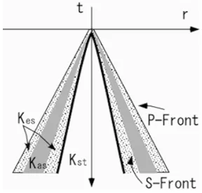
above. First, we recognize that the time dependence is similar in Eqs. (4) to (6); in other words, the time depen-dence is described only by two functions (ct/r)2−13/2 that the evaluation point(r,t)must be far behind the body-wave fronts in the causality cone, over which the discrete integration is carried out in Eq. (1). The causality cone can be divided into the following four domains according to the behavior of the integration kernel (Fig. 1):
(1)αt/r∼1 (immediately behind theP-wave front); (2)βt/r∼1 (immediately behind theS-wave front); (3) αt/r 1 andβt/r 1 (far behind both P- and S-wave fronts);
(4) αt/r 1 and βt/r < 1 (far behind the P-wave front, but before the arrival of theS-wave front.
While the exact integration kernelKes(.)[≡K(.)in Eq. (3)] should be used in the domains (1) and (2), the asymp-totic onesKas(.)andKst(.)can be used in the domains (3) and (4), as will be shown below, because of the satisfaction of the conditionγ =ct/r 1 there. Note that the bound-aries of integration domains (3) and (4) are dependent on space and time in contrast to the spatially independent one in the spectral BIE (Lapustaet al., 2000; Lapusta and Rice, 2003). In the spectral BIE, the integration kernel can be described in a time series and, consequently, a simple trun-cation in time can be effectively applied for the reduction of computation time in the stress evaluation. For non-planar faults, we cannot use such a truncation of kernels in time because of their dependence on both space and time.
2.2.2 Static asymptotic kernel valid for αt/r 1 and βt/r 1 We now derive the expression of the integration kernel asymptotically valid forαt/r 1 and
βt/r 1 in domain (3) mentioned in Section 2.2.1. We observe in Eqs. (4) to (6) that the dependence on time t is
Fig. 1. Four domains of integration corresponding to three kernels.
described by the two functions inIσpq(·):
A(t/r)=p3[(αt/r)2−1]3/2−[(βt/r)2−1]3/2,(11)
B(t/r)=p3(αt/r)2−1−(βt/r)2−1. (12)
If we employ the asymptotic expansions (9) and (10), we find that Eqs. (11) and (12) behave in the form forαt/r 1
We therefore obtain the asymptotic expressions ofIσpq(·)
(p,q = 1,2)valid forαt/r 1 and βt/r 1 in the
after substituting Eqs. (13) and (14) into Eqs. (4)–(6), where the other terms dependent on time t, that is, H(ζ) and Arccos(ζ ), can be discarded because the conditions
|H(ζ )| γ and|Arccos(ζ)| γ are satisfied for any real numbersγ 1.
We find in Eqs. (15) to (17) that Iσpq(·)is factorized into two terms dependent only on space or time. Equation (3) can therefore be reduced to a simple form:
=[Ist(x1+s/2,x2)−Ist(x1−s/2,x2)]t ≡Kst(x1,x2)t, (18)
where the subscriptσpq is omitted for brevity. We should note here that Kst(x1,x2) is independent of time t; the
subscriptst here denotes a function independent of time. The concrete expression forIst(.)is given by
Ist;σ11(x1,x2,t)≡ −
for each stress component. As will be shown below, the advantage of our approach is that we do not have to carry out the temporal integration if the asymptotic expression (18) is used.
Since the slipSi,n at thei-th line fault element andn-th
time step is related to the slip velocityDi,min the form:
Si,n =
n
m=0
Di,mt, (22)
the integration with respect to time can be carried out ana-lytically in Eq. (1), and we have
In this way, we can reduce the spatio-temporal integration into the spatial one because the integration can be carried out analytically with respect to time.
SinceKst(.)is independent of time,Kst(.)is expected to
be identical to the static integration kernel directly obtain-able from the static BIE (Andoet al., 2004). It is shown that this is actually the case: see Andoet al.(2004). In the following text, we refer to the above asymptotic integra-tion kernelKst(.)as the static asymptotic kernel. It should
be noted that the numerical computation of the exact ker-nels (Eqs. (4)–(6)) could cause a computer problem under a long-time condition since theP- andS-wave parts of the above integration kernels diverge ast3. However, this
diver-gence is removed by the use of the above static asymptotic kernels.
2.2.3 Dynamic asymptotic kernel valid forαt/r 1 and βt/r < 1 We next derive the asymptotic expres-sion for integration kernelKas(.) valid forαt/r 1 and
βt/r < 1 in domain (4) mentioned in Section 2.2.1. We are now able to employ the asymptotic expansions (9) and (10) associated with the P-wave only. We then obtain the asymptotic expressions for the function Iσaspq (p,q = 1,2)
It should be noted here again that each term is factorized into two terms dependent only on space or time. Attention should be given to the fact that Eqs. (24)–(26) involve the third-order terms in addition to the first-order ones on time t, so that both temporal and spatial integrations are required in Eq. (1). The requirement of temporal integration phys-ically means that the static equilibrium state has not been attained because theS-wave has not arrived yet. We refer to the asymptotic integration kernel given by Eqs. (24)–(26) as the dynamic asymptotic kernel taking account of the above property.
2.3 Efficient calculation of integration kernels
In this section we demonstrate that our method becomes highly efficient when the integration kernel is factorized into terms dependent only on space or time.
where we find that each term in the expansion ofK(.)is factorized into two terms dependent only on space or time; the subscriptσpqis omitted here for brevity.
In general, the integration kernel has the form of a dense matrix in the BIEM; consequently, the evaluation of the matrix elements becomes the numerically demanding part, in contrast with the finite element methods described by sparse matrices. The application of the above factorization of the integration kernel can reduce this numerical load significantly.
Let us try to evaluate a dense matrix of orderJ×M:
K =
⎛ ⎜ ⎝
K11 · · · K1M ... ... ...
KJ1 · · · KJ M ⎞ ⎟
⎠, (28)
where each element is assumed to denote an integration kernel, and the two subscripts denote the space node and time step, respectively. We find that the calculation time of the matrix is given by J ·M ·C1and that the memory
requirement is proportional toJ·M, whereC1is the average
calculation time of each matrix element. However, when each matrix element is factorized into terms dependent only on space or time, the matrix can be written in a form of vector product:
K =
⎛ ⎜ ⎝
F1
...
FJ ⎞ ⎟
⎠G1 · · ·GM
, (29)
where the calculation time is reduced to(J+M)·C2+J·M
and the required memory, which is now proportional to J +M, is also significantly reduced, where the constant C2 is the average calculation time of each element of the
vectors in Eq. (29). We can derive a relationC2∼1/100C1
by comparing the number of operations of floating points and internal functions (such as square root or trigonomet-ric functions) in Eqs. (4)–(6) with those in Eqs. (24)–(26), which means the reduction of calculation time by a fac-tor of 100. It should be noted that the computation time and memory requirement is further reduced when the static asymptotic kernel can be employed because then there is no contribution from terms dependent on time.
2.4 Representation of integration kernel for the anti-plane fault
A much simpler asymptotic expression of the integration kernel is obtained for the anti-plane fault than for the in-plane fault because of the contribution of theS-wave alone in the former. Following the above analysis of the in-plane fault, the causality cone can be divided into two domains, that is, at the vicinity of the S-wave front and outside of it. The exact and asymptotic kernels are employed in the former and latter domains, respectively.
The exact expressions for the function Iσpq(·) (p,q = 1,2)are written as
Iσ31(x1,x2,t)= − x2
πrH
t−r
β (βt/r)2−1, (30)
Iσ32(x1,x2,t)
=H(x1)H
t−|x2|
β
+π1sgn(x1)H
t− r
β
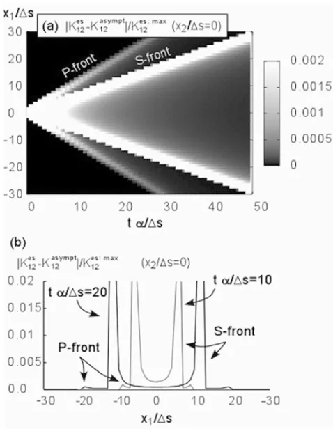
Fig. 2. Spatio-temporal distribution of error of asymptotic solution for the 12 components of the integration kernel atx2/s=0. (a) Distribution of error on the planex2 = 0. The areas in white have error values ranging from 0.002 to 0.6. The distribution of error is found to be approximated by hyperbolic functions near theP- andS-wave fronts. We therefore assume a hyperbolic function to describe the boundary between the domains where the exact or asymptotic kernels are used. (b) Temporal cross sections of error attα/s=10 and 20. Note that the tensile stress components, the 11 and 22 components, are identically zero on the planex2/s=0.
× ⎡ ⎣|x1|
r
(βt/r)2−1−arccos |x1|
(βt)2−x2 2
⎤ ⎦
(31)
(Tada and Madariaga, 2001). We find that the asymptotic expressions valid forβt/r 1 are given by
Iσ31(x1,x2,t)≈ −
β π
x2
r2t, (32)
Iσ32(x1,x2,t)≈
β
πsgn(x1)|
x1|
r2 t (33)
taking account of the asymptotic expansion (10). Since these asymptotic expressions are linear functions oft, the static asymptotic expressions referred to as Ias;σpq(.) (see Section 2.2) can be derived in the form:
Iσst31(x1,x2)= −
β π
x2
r2, (34)
Iσst32(x1,x2)=
β πsgn(x1)
|x1|
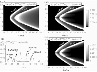
Fig. 3. Spatio-temporal distribution of the error of the asymptotic solution for the integration kernel atx2/s=10. Distributions of error for the 12, 11 and 22 components are shown in (a), (c) and (d), respectively, and an example of temporal cross sections of error is shown in (b) for the 12-component distribution. The spatio-temporal distribution and magnitude of error are found to be similar to those observed in the casex2/s=0 (Fig. 2), which implies that our method is also applicable to the analysis of non-planar faults with the same degree of accuracy.
2.5 Accuracy of the method and boundaries of the in-tegration domains
In this section, we first examine errors due to the employ-ment of the asymptotic kernels, using an in-plane fault as an illustrative example. Based on this error analysis, we deter-mine the boundaries of each integration domain where the asymptotic or exact integration kernel is used.
2.5.1 Spatio-temporal distribution of error We show the spatio-temporal distribution of error in order to check the accuracy of dynamic and static asymptotic repre-sentations (Figs. 2 or 3). Hereafter, we assume a Poisson solid, which isβ/α=1/√3. Here, the error is defined as the absolute value of the difference between the exact and asymptotic kernels divided by the maximum value of the exact kernel. The error is shown as a function of both time and space in Fig. 2(a), and as a function of space with time fixed in Fig. 2(b); the locations of source and array of re-ceivers are assumed to be coplanar. As clearly observed in these figures, the error is largest near the wave fronts and quickly decays with distance from the wave fronts, rapidly becoming less than 2×10⁻³.
The locations of the source and array of receivers are assumed to be non-coplanar (x2/s = 10) in Fig. 3. A
comparison of Figs. 2 and 3 reveals that the spatio-temporal distribution of error is similar, except for a difference due to the radiation pattern of elastic waves.
The practical significance of the above result of error analysis is worth noting. For analyses of arbitrarily oriented planar faults, we need integration kernels for the non-coplanar locations of the source and receiver. Since the degree of accuracy is almost the same in coplanar and non-coplanar distributions of source and array of receivers, it is fully expected that non-planar faults can be analyzed with
the same degree of accuracy as planar faults. This will actually be confirmed in Section 3.3.
Figures 2 and 3 show that the asymptotic kernels do not approximate the exact one very well directly behind the P- and S-wave fronts. This indicates that we have to use the exact kernels for this point onwards because the condition of asymptotic convergence is not satisfied, as shown in Section 2.2.3.
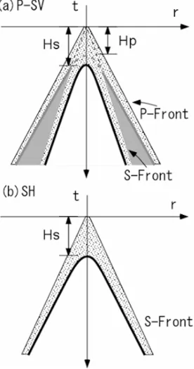
2.5.2 Definition of integration domains character-ized by different representations of the integration ker-nels We now define each integration domain where the asymptotic or exact integration kernel is used on the basis of the observations presented in Figs. 2 and 3 showing that the error is largest directly behind the fronts of theP- and S-waves and that the spatio-temporal distribution of errors appears to be hyperbolic. To be concrete, the exact ker-nels are employed in domains immediately behind the P -and S-wave fronts where the largest error is found in the asymptotic kernels, while the asymptotic kernels are used in domains where the error is smaller than a certain threshold. The boundaries of the domains are assumed to be described by hyperbolas that take the spatio-temporal distribution of error into account.
In practice, as shown in Fig. 4, the boundaries of integra-tion domains are defined near the wave fronts by the follow-ing two hyperbolic functions for the in-plane fault
t =
(r/α)2+H2
p,
t =(r/β)2+H2
s.
, (36)
The boundary is defined by the single function
t =
(r/β)2+H2
Fig. 4. Definition of integration domains and control parameters.
in the modeling of the anti-plane fault because of the con-tribution of the S-wave alone. The parameters Hp andHs
lie in the range 0 < Hc < Tmax (c = P or S), where
Tmax=NtandNis the number of total time steps in each
simulation. In conclusion, the exact kernels are assumed in the domains:
r/α≤t≤
(r/α)2+H2
p
r/β ≤t ≤(r/β)2+H2
s
(38)
for the in-plane fault and
r/β≤t≤
(r/β)2+H2
s (39)
for the anti-plane fault, respectively. A larger value of Hc/Tmax (c = p or s) implies that a larger domain is
assumed for the exact kernel; hence, a longer calculation time is required, although a higher accuracy is attained.
3.
Application to Fault Analyses
In this section, we first confirm the accuracy of our anal-yses on planar and non-planar faults. We then show that the use of a static asymptotic integration kernel, which charac-terizes our method, leads to the treatment of quasi-static and dynamic fault growth in a single numerical scheme. 3.1 Error in slip velocity
We generally try to obtain fault slip velocity on the as-sumption of traction applied on the fault in theoretical or numerical analyses of fault growth. If the BIEM is em-ployed in the analysis, we have to evaluate the convolution of the integration kernel and fault slip velocity in the past to obtain the fault slip velocity at a certain instance of time. Hence, when the asymptotic integration kernel is employed, the error tends to increase with the time step in the slip ve-locity because of the accumulation of error in the assumed
integration kernel. We now investigate how the error is ac-cumulated with the time step in comparison with the case when the exact integration kernel is used over the causality cone.
We assume a simple problem for this investigation of the behavior of the error: a rupture is nucleated at the origin and propagates bilaterally with a constant speed on a pla-nar fault (Section 3.2) or a non-plapla-nar fault (Section 3.3); The shear stress is assumed to drop suddenly by a constant value at the propagating fault tips. For numerical imple-mentation, the Courant-Friedrichs-Lewy (CFL) parameter is taken to be 0.5, and the temporal collocation points are chosen at the top of each unit time-step interval (i.e.et =1
following the definition of Tada and Madariaga, 2001). We adopt the following procedure to investigate how the error is generated during all of the time steps. The asymptotic ker-nels are employed at each time step for the domains deter-mined by the above-mentioned control parametersHc/Tmax
(c = α, β) in the causality cone (see Fig. 4). For each time step, Hc/Tmax is fixed at a certain value; this means
the domains for which the asymptotic kernels are assumed expand with increasing time. We consider the error as the difference between the two cases: only the exact kernels are used over the causality cones in one case, while both asymptotic and exact kernels are joined in the other case, as depicted in Fig. 4. In particular, as a measure of the error, we assume the relative difference of the two solutions av-eraged over the fault in time and space, which is given by
m
j|D
m,i
es −D
m,i as |/
m
j|D
m,i
es |, where D m,i es is the
slip velocity at them-th time step and thei-th fault element evaluated using only the exact kernel, while both exact and asymptotic kernels are used for the calculation of slip ve-locityDm,i
as . We study the dependences of error on the
con-trol parameters Hc/Tmax and on the computation time and
memory requirement below.
3.2 Accuracy of the analysis of planar fault
We first assume a planar fault for both in-plane and anti-plane faults. An example of slip velocity distribution and its dependence on the value of Hs/Tmaxis shown in Fig. 5
for the in-plane fault with Hs/Tmax =0.16 and 0.24. For
comparison purposes, we also show the solution obtained by assuming the exact kernel over the causality cone; such a solution is referred to in the following text as the exact solu-tion (note that “exact” refers only to the kernels and that the analysis is done numerically). This calculation shows that the dependence on the parameterHp/Tmaxis small enough
in the range 0.08 < Hp/Tmax < 0.2 and is negligible
in comparison to the effect of Hs/Tmax; consequently, the
value of Hp/Tmaxis fixed at 0.18 in the following
calcula-tions. As exemplified in Fig. 5(b), the slip velocity increases and is converged monotonically to the exact solution with increasingHs/Tmax. It should be noted that the short
wave-length oscillation observed in each curve is the error due to the discreteness of our calculation; it has nothing to do with the use of the asymptotic kernels.
The dependence of error on the required calculation time and amount of memory is shown in Fig. 6 for both in-plane and antiplane planar faults in the range 0.16< Hs/Tmax<
re-Fig. 5. Slip velocity for a self-similar in-plane fault. (a) Configuration of the assumed model. The fault tip velocity is assumed to be 80% of the speed of theS-wave. (b) Spatial distribution of slip velocities at time stepN = 100; two different values are assumed for the control parameterHs/Tmax. The result obtained in the analysis in which only the exact kernel is used over the causality cone is also shown for com-parison. Shown here is the non-dimensional slip velocity that is given by the slip velocity divided byασo/μ, whereσois the shear stress drop assumed on the fault.
Fig. 6. Dependence of error on calculation time and memory required in the analysis of planar fault. Solid and dotted black curves denote the calculation time and memory requirement in the analysis of in-plane fault, respectively; solid and dotted gray curves are for the anti-plane fault.
quirement is enhanced, which is associated with the expan-sion of the domains where the exact kernels are assumed. For example, if a 10% error is allowed in the modeling of planar fault, the reductions in the calculation time and the memory requirement are about 45% and 60%, respectively, in comparison to the exact solution. Similarly, if a 3% error is allowed whenHs/Tmax∼0.48, the reductions are about
25% and 45%, respectively.
Figure 6 also shows that the error is much smaller in the simulation of the anti-plane fault than in that of the in-plane fault. This difference occurs because we can employ only the exact and static asymptotic kernels in the calculation due to the contribution of theS-wave only, as mentioned in Section 2.4. The calculation time and memory requirement (60% and 75% reductions for a 3% error, respectively) are also much smaller in the simulation of the anti-plane fault for the same reason. In addition, it should be mentioned that the reduction in calculation time in the analysis of
in-Fig. 7. Dependence of error on calculation time required in the analysis of non-planar fault. The black curve denotes the case for the non-planar fault. The gray curve denotes the error for the planar fault. Fault geometries are shown in the inset, whereLdenotes the whole length of each fault. In both examples, the fault tip velocity is assumed to be 80% of theS-wave speed, and the same shear stress drop is assumed along each fault trace.
plane fault will be comparable to that found in the analysis of anti-plane fault as the ratioβ/αapproaches unity since the domain between the fronts of the P- andS-wave, over which the most time-consuming convolution has to be car-ried out, shrinks in the causality cone (see Fig. 1).
Figure 5(b) implies that a higher accuracy is attained only if the amplitude of the longer wavelength variation is increased slightly because shorter wavelength components are reproduced well, even for smaller values of Hc/Tmax.
Since longer wave components are associated with slow fault motion, while shorter wave components are associated with fast fault motion, it is suggested that the deficit in the longer wavelength components are recovered by retaining higher order terms in the asymptotic approximation at the long wavelength limit. An example of the correction proce-dure is shown in Appendix A.
3.3 Applicability to non-planar fault analyses
Let us explore the applicability of our method to the analysis of non-planar faults under the assumption that one of the simplest models has a feature of non-planar faults; as such, a non-planar fault with an abrupt bend is assumed, as illustrated in the inset of Fig. 7. The error is plotted as a function of calculation time in Fig. 7; the error for a planar fault is also shown for comparison. As clearly observed, the dependence of error on the calculation time is almost the same for the two faults. The memory requirement is found to have a similar dependence.
The above consideration indicates that our method can treat non-planar faults with the same degree of accuracy as planar faults.
4.
A Further Reduction in Computation Time and
Required Memory by the Repetitive Use of
In-tegration Kernels
The integration kernels in the elasto-dynamic BIEM have translational symmetry with respect to time
K(x,t;ξ, τ)=K(x,t−τ;ξ,0). (40)
Fig. 8. Reduction of calculation time by the repetitive use of kernels stored in computer memory. The dependence of calculation time on the time step is reduced fromN2toN. The exact kernel is used over the causality cone in each example.
the property (40) is employed; a self-similar in-plane fault is assumed in the calculation. The kernels stored in computer memory are used repeatedly in one example, and the ker-nels are calculated at each time step in the other example; the calculation times are shown to be dependent onN and N2in both examples. Hence, the employment of property
(40) is found to lead to a significant reduction in calcula-tion time, and a large-scale calculacalcula-tion will be facilitated by our method. This reduction in calculation time can be un-derstood as follows; as mentioned earlier, the time required for the calculation of the integration kernel is proportional ton2 at time stepn. Hence, the total calculation time is proportional to N3 ∼ nN=1n2if the integration kernel is
calculated at each time step, whereNis the number of total calculation steps. However, this summation does not con-tribute to the calculation time when the stored kernels are employed repeatedly; in this latter case, the calculation time is reduced to the order ofN2.
5.
Note on the application to modeling of
earth-quake cycles
We briefly explain how to apply our efficient BIEM to the modeling of an earthquake cycle consisting of both quasi-static and dynamic phases. If we use a striking feature of our BIEM that the contribution from far behind theS-wave front is represented only by the spatial convolution of slip and the static asymptotic integration kernel, then we can efficiently simulate both phases in a single scheme with high accuracy. Although such a numerical scheme has been developed for planar faults (Lapusta and Rice, 2003), our method has an advantage that both planar and non-planar faults are treated similarly.
Figure 9 schematically illustrates how to treat quasi-static and dynamic processes in a single scheme. The ruptured area (shaded zone) is assumed to expand quasi-statically at the initial stage and then its growth is gradually acceler-ated to a dynamic one. Three collocation points (marked by crosses) corresponding to three typical growth stages are arbitrarily assumed on the fault, and the causality cone asso-ciated with each collocation point is illustrated; each causal-ity cone is divided into integration domains according to the
Fig. 9. Schematic illustration of unified treatment of dynamic and quasi-static fault ruptures in a single earthquake cycle. Three causal-ity cones are shown in individual stages of an earthquake cycle where the spatio-temporal expansion of the ruptured area is shown by the grey zone. Three different line segments shown on the right schematically denote the discrete time intervalstto be assumed at each stage. Refer to text for the description ofT∗.
difference in the representation of kernel (refer to Fig. 1 for the color-coding of integration domains). It should be noted here that the exact and dynamic asymptotic kernels must be employed in the dotted and gray domains, while the static one is used on the thick curve.
As schematically illustrated in Fig. 9, the temporal in-tegration is required only in the analysis of the dynamic phase. The fact that the range of temporal integrationT∗ is far less than the time required for the analysis of an earth-quake cycle is important for the efficient calculation. Since the upper limit of the temporal integration can be truncated atT∗, the time required for the calculation of the dynamic phase is independent of the number of total steps for the calculation of earthquake cycle.
It is also important for the rapid calculation in our method that we can vary the time stept.; we can assume much larger value for t. in the quasi-static phase than in dy-namic phase. While we have to assume a sufficiently small magnitude fort in the dynamic phase, the integration is reduced to the spatial one far behind theS-wave front. This facilitates the fast calculation.
6.
Conclusions
dependent on space or time, resulting in the numerical treat-ment being fully efficient. No temporal terms are shown to contribute to the kernels far behind theS-wave front, so that any further speed-up of the calculation is attained because only the spatial integration is necessary. We show that, in a dynamic analysis, if a 3% error is allowed for the slip rate, the computation time and memory requirement are reduced by 25% and 45%, respectively, in an in-plane fault case; in an anti-plane fault case, the respective reductions are 60% and 75%. The calculation time is further reduced if we use the translational symmetry of the integration kernel with re-spect to time. It should also be noted that our method of analysis is useful even for earthquake rupture whose growth rate is much slower than the speed of theS-wave.
We have therefore demonstrated that the present method is a powerful numerical tool to simulate an entire earth-quake cycle with a more realistic non-planar fault model in a single scheme. We conclude with a remark that it can be extended to 3-D problems without large difficulties al-though only 2-D cases are validated here.
Acknowledgments. The authors greatly appreciate beneficial comments by Raul Madariaga and an anonymous referee. R. A. is supported by a Japan Society for Promotion of Science (JSPS) Postdoctoral fellowship in 2005–2007. The work was additionally supported by the Earthquake Research Institute cooperative pro-gram (N.K. and T.Y.) and the DaiDaiToku Project, MEXT, Japan (N.K.).
Appendix A. Improvement of accuracy by
retain-ing a higher order term
We now show how the accuracy of the calculation is improved by retaining a higher order term in the asymptotic expansion. Following the procedure shown in Section 2.2.2, the contribution from the term on the order ofγ−1G(σ−i j1)is obtained to each stress component in the form
G(σ−111)(x1,x2,t)= −(
3p2+1)(p2−1)
2π
x2
βt, (A.1)
G(σ−221)(x1,x2,t)=
(p2−1)2
2π x2
βt, (A.2)
G(σ−121)(x1,x2,t)=(
p4−1) 2π
x1
βt. (A.3)
We find that the term on the order oft−1appears in each
equation, so that the asymptotic expression is no longer time-independent. Hence, in order to retain the useful static property of the static asymptotic expression, we assume that the slip velocity is constant D at each fault element throughout the slip duration only when the contributions (A.1) to (A.2) are taken into account; this enables us to carry out the temporal convolution analytically for the terms proportional tot−1.
The temporal convolution of the integration kernel and constant slip velocityDcrr can be carried out in the form:
to−Tstart
to−Tfinal
K(x1,x2, τ)Dcrrdτ
=([f(−1)(x1+s/2,x2) − f(−1)(x1−s/2,x2)]Dcrr
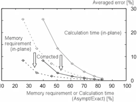
Fig. A.1. Slip velocities simulated with (gray curve) and without (dot-ted curve) the correction terms obtained at time step N = 100;
Hs/Tmax = 0.08 is assumed in the calculation. The exact solution (black curve) is shown for reference. Refer to the caption of Fig. 5 for the unit of non-dimensional slip velocity.
Fig. A.2. Dependence of error on required calculation time and memory. The two solid curves denote calculation time and memory requirement, respectively, when the correction term is applied; note that the accuracy is improved by the introduction of the correction term (compared with gray curves).
×
to−Tstart
to−Tfinal
{1/(τ+t)−1/τ}dτ
=([f(−1)(x1+s/2,x2) − f(−1)(x1−s/2,x2)]Dcrr
×log
(
to−Tfinal){(to−(Tstart+t)}
(to−Tstart){to−(Tfinal+t)}
,
(A.4)
wheretoandTstartare current time and the time of slip
on-set, respectively, and the asymptotic expression for the ker-nelK is assumed to be valid in the range 0 <to−Tstart <
τ <to−Tfinal =
(r/β)2+H2
s; see Eq. (37). The
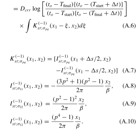
func-tion f(−1)(·)is obtained from spatial term in Eqs. (A.1)– (A.3). We finally find that the following correction term Rσpq(to,Tstart,Tfinal)should be added to the spatial convolu-tion term with the asymptotic static kernel as
Kσstpq(x1−ξ,x2)S(ξ)dξ +Rσpq(to,Tstart,Tfinal), (A.5)
where
=Dcrrlog
(to−Tfinal){(to−(Tstart+t)}
(to−Tstart){to−(Tfinal+t)}
×
Kst(−;σ1)pq(x1−ξ,x2)dξ (A.6)
with
Kst(−;σ1)pq(x1,x2)=[I (−1)
st;σpq(x1+s/2,x2)
−Ist(−;σ1pq)(x1−s/2,x2)] (A.7)
Ist(−;σ1)
11(x1,x2)= −
(3p2+1)(p2−1)
2π
x2
β , (A.8)
Ist(−;σ122)(x1,x2) = (
p2−1)2
2π x2
β, (A.9)
Ist(−;σ112)(x1,x2)=
(p4−1)
2π x1
β. (A.10)
We now investigate how the accuracy of the calculation is improved by the addition of the correction terms in a simu-lation of fault growth; a self-similar in-plane fault studied in Fig. 5 is assumed to be once again one of the simplest mod-els. The distribution of slip velocity on the fault is shown in Fig. A1 for the case of Dcrr/(ασ/μ) = 4; the exact solution is also illustrated as reference. In comparison with the solutions with and without the correction term, the accu-racy is improved by the introduction of the correction term. We also investigate the dependence of error on the calcula-tion time and memory requirement (see Fig. A2) and find that the accuracy is improved when calculation time and re-quired memory are fixed (e.g., the reduction of 40% in the calculation time with 3% error). The value of Dcrr is
de-termined by trial and error in the calculation here so that the error may take the minimum value when the calculation time is 60% of the time required for the calculation of the exact solution.
As shown above, the introduction of a higher order cor-rection term is found to contribute to the increase in the accuracy of the analysis of self-similar fault. However, the development of a generally applicable method to improve the accuracy is a future task.
References
Ando, R., T. Tada, and T. Yamashita, Dynamic evolution of a fault system through interactions between fault segments,J. Geophys. Res.,109(B5), doi:10.1029/2003JB002665, 2004.
Aochi, H. and E. Fukuyama, Three-dimensional nonplanar simulation of the 1992 Landers earthquake,J. Geophys. Res.,107(B2), doi:10.1029/ 2000JB000061, 2002.
Aochi, H., R. Madariaga, and E. Fukuyama, Constraint of fault parameters inferred from nonplanar fault modeling,Geochem. Geophys. Geosyst.,
4, 2003.
Cochard, A. and R. Madariaga, Dynamic Faulting under Rate-Dependent Friction,Pure Appl. Geophys.,142(3–4), 419–445, 1994.
Fukuyama, E., C. Hashimoto, and M. Matsu’ura, Simulation of the transi-tion of earthquake rupture from quasi-static growth to dynamic propa-gation,Pure Appl. Geophys.,159(9), 2057–2066, 2002.
Kame, N. and T. Yamashita, A new light on arresting mechanism of dy-namic earthquake faulting,Geophys. Res. Lett., 26(13), 1997–2000, 1999a.
Kame, N. and T. Yamashita, Simulation of the spontaneous growth of a dynamic crack without constraints on the crack tip path,Geophys. J. Int.,139(2), 345–358, 1999b.
Kame, N. and T. Yamashita, Dynamic branching, arresting of rupture and the seismic wave radiation in self-chosen crack path modelling, Geo-phys. J. Int.,155(3), 1042–1050, 2003.
Kame, N., J. R. Rice, and R. Dmowska, Effects of prestress state and rupture velocity on dynamic fault branching,J. Geophys. Res.,108(B5), doi:10.1029/2002JB002189, 2003.
Kato, N., Interaction of slip on asperities: Numerical simulation of seis-mic cycles on a two-dimensional planar fault with nonuniform frictional property, J. Geophys. Res., 109(B12), doi:10.1029/2004JB003001, 2004.
Lapusta, N. and J. R. Rice, Nucleation and early seismic propagation of small and large events in a crustal earthquake model,J. Geophys. Res.,
108(B4), doi:10.1029/2001JB000793, 2003.
Lapusta, N., J. R. Rice, Y. Ben-Zion, and G. T. Zheng, Elastodynamic analysis for slow tectonic loading with spontaneous rupture episodes on faults with rate- and state-dependent friction, J. Geophys. Res.,
105(B10), 23765–23789, 2000.
Tada, T. and R. Madariaga, Dynamic modelling of the flat 2-D crack by a semi-analytic BIEM scheme,Int. J. Numer. Methods Eng.,50(1), 227– 251, 2001.
Tada, T. and T. Yamashita, Non-hypersingular boundary integral equations for two-dimensional non-planar crack analysis,Geophys. J. Int.,130(2), 269–282, 1997.
Tse, S. T. and J. R. Rice, Crustal Earthquake Instability in Relation to the Depth Variation of Frictional Slip Properties,J. Geophys. Res.,91(B9), 9452–9472, 1986.