doi:10.1155/2009/938492
Research Article
Stability Results for a Class of Difference Systems
with Delay
Eva Kaslik
Department of Mathematics and Computer Science, West University of Timisoara, Bd. C. Coposu 4, 300223 Timisoara, Romania
Correspondence should be addressed to Eva Kaslik,[email protected]
Received 2 November 2009; Accepted 13 December 2009
Recommended by Mariella Cecchi
Considering the linear delay difference systemxn1 axn Bxn−k, wherea∈0,1,Bis a
p×preal matrix, andkis a positive integer, the stability domain of the null solution is completely characterized in terms of the eigenvalues of the matrixB. It is also shown that the stability domain becomes smaller as the delay increases. These results may be successfully applied in the stability analysis of a large class of nonlinear difference systems, including discrete-time Hopfield neural networks.
Copyrightq2009 Eva Kaslik. This is an open access article distributed under the Creative Commons Attribution License, which permits unrestricted use, distribution, and reproduction in any medium, provided the original work is properly cited.
1. Introduction
In this paper, we will characterize the stability region of the null solution for the following class of linear delay difference systems:
xn1 axn Bxn−k ∀n≥k, 1.1
wherea∈0,1,Bis ap×preal matrix, andkis a positive integer.
Similar linear difference systems have been recently investigated by Levitskaya1
focusing on the special casea1and by Kipnis and Komissarova2 studying the special casea −1. Two-dimensional systems of this form have been thoroughly investigated by Matsunaga, in the casea 13,4and in the general casea ∈R5. The common starting point of all these results is the well-known papers of Kuruklis 6 and Papanicolaou 7, which focus on the scalar difference equation
wherea, b ∈Randk∈N∗. A more recent discussion of the stability properties of this scalar difference equation, based on relatively simple arguments, is presented in 8. As for the nondelayed casek0, we refer to the recent paper in9and the references therein.
System 1.1 can be regarded as the linearization at the origin of the following nonlinear delay difference system:
xn1 Fxn,xn−k ∀n≥k, 1.3
where the functionF :Ω×Ω → Ω with0∈Ω⊂RpsatisfiesF0,0 0,Dx
1F0,0 a·Id
where Id denotes thep-dimensional identity matrix, andDx2F0,0 B.
In particular, discrete-time delayed Hopfield-type neural networks described by
xn1 axn Tgxn−k ∀n≥k 1.4
belong to the class of nonlinear difference systems1.3. In this context,a∈0,1is the self-regulating parameter of the neurons,T ∈ Rp×p is the interconnection matrix,g
i : R → R,
i ∈ {1,2, . . . , p} are the neuron input-output activation functions satisfyinggi0 0, and
g : Rp → Rpis defined bygx g
1x1, g2x2, . . . , gpxpT. In this framework, stability
and bifurcation results have been obtained in10for the two-dimensional case, in11for the case of a single-directional ring of four neurons, and in12for a bidirectional ring ofp
neurons. Moreover, coexistence of chaos and periodic orbits for a network of this type with two identical neurons and no self-connections has been observed in13.
The stability of the null solution of system1.1will be investigated by analyzing the distribution of the roots of the corresponding characteristic equation with respect to the unit circle. Based on2, Corollary 2.2,1.1is asymptotically stable if and only if all roots of the equation
detB−zkz−aI0 1.5
lie inside the unit disk. This means thatzis a root of the characteristic equation of1.1if and only ifzkz−ais an eigenvalue of the matrixB.
In the followings, we will denote byλi,i∈ {1,2, . . . , p}the eigenvalues ofB. Based on
the previous remark, we obtain that the characteristic equation of1.1is
p
i1
zkz−a−λi
0. 1.6
The null solution of1.1is asymptotically stable if and only if all the roots of the characteristic equation 1.6 are inside the unit circle. Therefore, in order to characterize the asymptotic stability of the null solution of1.1, we first need to analyze the distribution of the roots of the polynomialPλz zkz−a−λ, whereλis a complex parameter, with respect to the unit
2. The Roots of the Polynomial
P
λz
z
kz
−
a
−
λ, λ
∈
C
In the followings, we will consider the following two important functions:
ca,kθ cosk1θ−acoskθ,
sa,kθ sink1θ−asinkθ,
2.1
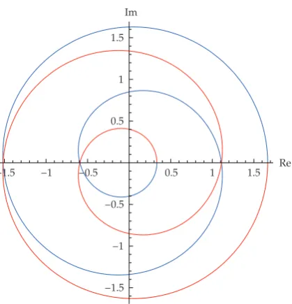
and the curveΓin the complex plane given by the following parametric equation:
Γ:uθ ca,kθ isa,kθ, θ∈−π, π. 2.2
Lemma 2.1. Letk∈Nanda∈0,1. The functionsa,khas exactlyk2roots in the interval0, π, more precisely, as follows:
iθa,k0 0is a root,
iiifk ≥1, then there is one rootθja,k in every interval2j−1π/2k1, jπ/k1⊂
j−1π/k, jπ/k,j ∈ {1,2, . . . , k}, iiiθk1
a,k πis a root.
Moreover,−1jsa,kθ>0for anyθ∈θa,kj , θja,k1,j ∈ {0,1, . . . , k}.
Proof. Obviously, 0 andπare solutions of the equationsa,kθ 0 for anyk∈N.
Consideringk ≥ 1, on the intervalj−1π/k, jπ/k,j ∈ {1,2, . . . , k}, the equation
sa,kθ 0 becomes
sink1θ
sinkθ a. 2.3
The functionh:j−1π/k, jπ/k → Rdefined byhθ sink1θ/sinkθis differentiable and
hθ k1cosk1θsinkθ−kcoskθsink1θ
sin2kθ
k1sin2k1θ−sinθ−ksin2k1θsinθ
2sin2kθ
sin2k1θ−2k1sinθ
2sin2kθ .
2.4
Therefore, the sign ofhθdepends on the sign ofgθ sin2k1θ−2k1sinθ. We have
gθ 2k1cos2k1θ−cosθ −22k1sink1θsinkθ. 2.5
One can easily verify that the only root ofgin the intervalj−1π/k, jπ/kisθjπ/k
is decreasing on the intervalj−1π/k, θand increasing onθ, jπ/k. Asgj−1π/k
−2ksinj−1π/k ≤ 0 andgjπ/k −2ksinjπ/k ≤ 0, it results thatgθ < 0 for any
θ∈j−1π/k, jπ/k.
Hence, the functionhis strictly decreasing on the intervalj−1π/k, jπ/k. Hence, the equationsa,kθ 0 has a single rootθja,kin the intervalj−1π/k, jπ/k. Moreover, as
wherehis the function defined in the proof ofLemma 2.1. We have shown thathis strictly decreasing on the interval j−1π/k, jπ/k; hence, the equation ca,kθ 0 has a single root on the intervalj −1π/k, jπ/k. Moreover, as hθa,kj a,hjπ/k 1 0 and
Moreover, forj∈ {0,1, . . . , k}we have Remark 2.3. Properties of the curveΓdefined by2.2:
awe can easily see that
Therefore, asθincreases from−πtoπ, the corresponding pointuθfrom the curve
Γmoves anticlockwise around the origin;
dthe curveΓintersects the real axis at the points
uθja,kca,k
θja,k −1j
1a2−2acosθj
a,k, j∈ {0,1, . . . , k1}, 2.15
which are at the same time the intersection points of the curve piecesΓ|−π,0and
Γ|0,π.
In what follows, we will consider the following curve pieces:
Γj
a,k Γ|−θja,k,−θja,k−1∪θj−1 a,k,θ
j
a,k, j ∈ {1,2, . . . , k1}. 2.16
Based on the previous remarks, one can easily see that these are closed curves.
For everyj ∈ {1,2, . . . , k1}, letΔja,k denote the domainopen and connected set, containing the originof the complex plane inclosed by the curveΓja,k.
Remark 2.4. For the curvesΓja,kand the inclosed domainsΔja,k, the following properties hold:
a Γja,k∩Γja,k1{ca,kθa,kj }for anyj∈ {1,2, . . . , k},
b∂Δja,k Γja,kfor anyj ∈ {1,2, . . . , k1}here,∂Sdenotes the boundary of the setS;
c Δ1
a,k⊂Δ2a,k ⊂ · · · ⊂Δk
1
a,k.
Using all these preliminary notations and results, the following proposition is obtained.
Proposition 2.5. Considering the polynomialPλz zkz−a−λ,λ∈C, the following hold.
aIfλ∈Δ1
a,k, then all roots of the polynomialPλzare inside the unit circle.
bIfλ∈Δja,k\Δja,k−1(withj∈ {2,3, . . . , k1}), then the polynomialPλzhas exactlyk−j2 roots inside the unit circle andj−1roots outside the unit circle.
cIfλ∈C\Δk1
a,k, then all roots of the polynomialPλzare outside the unit circle.
dIfλ∈Γja,k\ {ca,kθa,kj−1, ca,kθja,k}(withj ∈ {1,2, . . . , k1}), then the polynomialPλz has exactly one simple root on the unit circle,k−j1roots inside the unit circle andj−1
roots outside the unit circle.
eIfλca,kθa,kj ,j ∈ {1,2, . . . , k}, then the polynomialPλzhas exactly two simple roots
on the unit circle,k−jroots inside the unit circle, andj−1roots outside the unit circle. fIfλca,kθa,k0 1−a, then the polynomialPλzhas the simple rootz1on the unit
circle andkroots inside the unit circle.
gIfλca,kθa,kk1 −1k11a, then the polynomialPλzhas the simple rootz−1 on the unit circle andkroots outside the unit circle.
Proof. The polynomialPλzhas a rootzeiθ,θ∈−π, πon the unit circle if and only if
λeikθeiθ−ac
a,kθ isa,kθ, 2.17
that is, if and only ifλ∈Γ.
Furthermore, due to the properties of the curve Γ stated in Remark 2.3, we easily obtain that the polynomial Pλz has a unique root on the unit circle if and only if λ ∈ Γ\ {ca,kθ1a,k, ca,kθ2a,k, . . . , ca,kθa,kk }. We also obtain that ifλ ca,kθa,kj ,j ∈ {1,2, . . . , k},
then the polynomialPλzhas exactly two roots on the unit circle, namely, z eiθ j a,k and
ze−iθja,k.
Moreover, if the polynomialPλzhas a root on the unit circle, then this root is simple.
Indeed, assuming that there existsθ∈−π, πsuch thatzeiθis a root ofP
λzandPλz k1zk−akzk−10, we obtain thats
a,kθ ca,kθ 0. But we can easily see that
sa,kθ2ca,kθ2 k12a2k2−2akk1cosθ≥k12a2k2−2akk1
k1−ak2>0,
2.18
and hence, a contradiction is obtained.
To provea, we will use the argument principle for the investigation of the roots of the polynomialPλz zkz−a−λ. In other words, we will study the increase of the argument
ofPλzalong the unit circle. Consider the function
Gθ, λ Pλ
eiθeikθeiθ−a−λuθ−λ, 2.19
whereuθ ca,kθ isa,kθ. We will estimate the increase of the argument ofGθ, λasθ
increases from−πtoπ.
FromRemark 2.3, we know that|uθ|is strictly decreasing on the interval−π,0and increasing on the interval0, π, and asθ increases from−π toπ, the corresponding point
uθmoves anticlockwise around the origin. Moreover,Remark 2.3provides that the locus of
uθintersects the real axis 2k1times asθincreases on the interval−π, π. Hence, the increase of the argument ofuθasθincreases from−πtoπis 2k1πseeFigure 1.
The locus ofGθ, λis obtained by the translation of the locus ofuθby the vector
−Reλ,−Imλ. Ifλlies inside the domainΔ1a,k, then the increase of the argument ofGθ, λ
is the same as the increase of the argument of uθ, that is, it is equal to 2k1π. The argument principle provides that all the roots of the polynomial Pλz are inside the unit
circle, andais proved.
Letj ∈ {1,2, . . . , k1}. The next step of the proof is to show that when the complex
parameterλ λ1iλ2 leaves the domainΔja,k by crossing its boundaryΓja,k at a valueλ
ca,kθisa,kθ, withθ∈−θja,k,−θa,kj−1∪θja,k−1, θja,k, the rootzzλof the polynomialPλz,
0.5 1 1.5
In the following computations, we rely on the fact that the roots of the polynomial
Pλzwhich lie on the unit circle are simple.
Aszk1−azkλ
1iλ2andzk1−azkλ1−iλ2, differentiating with respect toλ1and then with respect toλ2, we obtain
We compute the directional derivative of|z|2atλ c continuous dependence of the roots of the polynomialPλzon the parameterλ, guarantees
the validity of the statementsb–gand completes the proof.
3. Stability Results
3.1. Characterization of the Stability Domain
Based on the results presented in the previous section and the characteristic equation1.6, the following main result is obtained.
Proposition 3.1. The null solution of system 1.1 is asymptotically stable if and only if all eigenvalues of matrixBbelong to the domainΔ1
a,k of the complex plane inclosed by the closed curve Γ1
Remark 3.2. The domainΔ1a,k can be expressed as
Δ1
a,k
λ∈C : ca,k
θ1a,k<Reλ<1−a ,|Imλ|< ha,kReλ
, 3.2
whereha,k sa,k ◦ca,k−1 andca,k−1 denotes the inverse of the restriction ofca,k to the interval 0, θ1a,k.
3.2. Dependence of the Stability Domain on the Delay
Proposition 3.3. As the delaykincreases, the stability domain becomes smaller, that is, the domains Δ1
a,ksatisfy
Δ1
a,k1⊂Δ1a,k for anyk∈N. 3.3
IfD0,1−adenotes the open disk of the complex plane, centered at the origin, of radius1−a, one has
∞
k0
Δ1
a,k D0,1−a. 3.4
Proof. Letk∈N. Based onRemark 3.2, the proof of the fact thatΔ1
a,k1 ⊂Δ1a,kwill consist of
the following steps.
Step 1. We will prove thatca,kθ1a,k < ca,k1θ1a,k1. Sinceca,kθ1a,k −
1a2−2acosθ1
a,k,
this reduces to show thatθ1
a,k1< θ1a,k.
Indeed, assuming the contrary that is, θ1a,k < θa,k1 1 and taking into account that
sa,k1θ > 0 for anyθ ∈ 0, θa,k1 1, it follows thatsa,k1θ1a,k > 0. On the other hand, we can easily see that
sa,k1θ sink2θ−asink1θsa,kθcosθca,kθsinθ 3.5
and hence,
sa,k1
θ1a,kca,k
θa,k1 sinθ1a,k<0. 3.6
Step 2. We will prove thatha,k1t< ha,ktfor anyt∈ca,k1θa,k1 1,1−a. Since
ca,kθ2sa,kθ21a2−2acosθ, 3.7
makingθc−1
a,kt, it follows that
ha,kt21a2−t2−2acosc−a,k1t. 3.8
Therefore, in order to prove thatha,k1t < ha,kt, it is sufficient to prove that c−a,k1 1t < c−1
a,ktfor anyt∈ca,k1θa,k1 1,1−a. Sinceca,kis decreasing on0, θ1a,k, this is equivalent to
show thatca,k1θ< ca,kθfor anyθ∈0, θa,k1 1. Indeed, for anyθ∈0, θa,k1 1we have
ca,k1θ cosk2θ−acosk1θca,kθcosθ−sa,kθsinθ < ca,kθ. 3.9
Finally, we will prove that∞k0Δ1
a,kD0,1−a.
We remark that D0,1−a ⊂ Δ1
a,k, for any k ∈ N. Indeed, it is easy to see that if λ ∈ ∂Δ1a,k Γa,k1 , there existsθ ∈ −θ1a,k, θa,k1 such that λ ca,kθ isa,kθ, and hence,
|λ|√1a2−2acosθ≥1−a. Thereforeλ /∈D0,1−aand it follows thatD0,1−a⊂Δ1
a,k.
We obtain thatD0,1−a⊂∞k0Δ1a,k. On the other hand, ifλ∈∞k0Δ1
a,k, then it follows fromRemark 3.2that
ca,k
θ1a,k<Reλ<1−a, |Imλ|< ha,kReλ ∀k∈N. 3.10
From the first inequality, since c−a,k1 is decreasing see Lemma 2.2, it follows that 0 < c−1
a,kReλ< θa,k1 . From the second inequality, we obtain
|λ|2Reλ2Imλ2< Reλ2ha,kReλ21a2−2acos
c−1
a,kReλ
<1a2−2acosθ1
a,k,
3.11
and hence
|λ|<
1a2−2acosθ1
a,k ∀k∈N. 3.12
FromLemma 2.1we know that 0 < θ1
a,k < π/k1, and hence, limk→ ∞θ1a,k 0. Passing to
the limit whenk → ∞in the previous inequality, we obtain that|λ|< 1−a, and therefore,
λ∈D0,1−a. It results that∞k0Δ1a,k⊂D0,1−aand the proof is complete.
0.2 0.2
0.4
−0.2
−0.4
−0.6
−0.8
−1
−0.2
−0.4 Im
Re
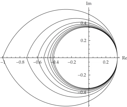
Figure 2:The stability domains fora2/3 andk∈ {1,2, . . . ,8}. We haveΔ1
a,8⊂Δ1a,7⊂ · · · ⊂Δ1a,2⊂Δ1a,1.
3.3. Some Particular Cases
Corollary 3.4. If all the eigenvalues of the matrix B are real, then the null solution of system 1.1 is asymptotically stable if and only if all eigenvalues of matrix B belong to the interval −1a2−2acosθ1
a,k,1−a.
For example, the previous corollary covers the case whenB is a symmetric matrix. In particular, for the 1-dimensional case p 1 we obtain the result of Kuruklis6and Papanicolaou7, whena ∈ 0,1. For the 2-dimensional case p 2, if the matrixBhas two real eigenvalues, then we obtain the result of Matsunaga5, whena ∈ 0,1. On the other hand, if the matrixB∈R2×2has two complex eigenvalues, then we obtain the following simple formulation.
Corollary 3.5. In the case of a 2-dimensional system of the form1.1, where the matrixBhas two complex conjugated eigenvaluesλ1,2 β1±iβ2, the null solution is asymptotically stable if and only if
−1a2−2acosθ1
a,k< β1 <1−a, β2< ha,k
β1
, 3.13
whereha,ksa,k◦c−a,k1 andca,k−1 denotes the inverse of the restriction ofca,kto the interval0, θa,k1 .
4. Conclusions and Future Directions
in the stability analysis of many nonlinear discrete-time dynamical systems arising from practical problems, such as discrete-time Hopfield neural networks. Investigating the bifurcations occurring in such nonlinear dynamical systems at the boundary of the stability domain may constitute a direction for future research.
References
1 I. S. Levitskaya, “A note on the stability oval forxn1xnaxn−k,”Journal of Difference Equations and
Applications, vol. 11, no. 8, pp. 701–705, 2005.
2 M. Kipnis and D. Komissarova, “Stability of a delay difference system,” Advances in Difference Equations, vol. 2006, Article ID 31409, 9 pages, 2006.
3 H. Matsunaga, “A note on asymptotic stability of delay difference systems,”Journal of Inequalities and Applications, vol. 2005, no. 2, pp. 119–125, 2005.
4 H. Matsunaga, “Exact stability criteria for delay differential and difference equations,” Applied Mathematics Letters, vol. 20, no. 2, pp. 183–188, 2007.
5 H. Matsunaga, “Stability regions for a class of delay difference systems,” inDifferences and Differential Equations, vol. 42 ofFields Institute Communications, pp. 273–283, American Mathematical Society, Providence, Ri, USA, 2004.
6 S. A. Kuruklis, “The asymptotic stability ofxn1−axnbxn−k 0,”Journal of Mathematical Analysis
and Applications, vol. 188, no. 3, pp. 719–731, 1994.
7 V. G. Papanicolaou, “On the asymptotic stability of a class of linear difference equations,”Mathematics Magazine, vol. 69, no. 1, pp. 34–43, 1996.
8 S. S. Cheng and Y.-Z. Lin, “Exact stability regions for linear difference equations with three parameters,”Applied Mathematics E-Notes, vol. 6, pp. 49–57, 2006.
9 B. Zheng and L. Wang, “Spectral radius and infinity norm of matrices,”Journal of Mathematical Analysis and Applications, vol. 346, no. 1, pp. 243–250, 2008.
10 E. Kaslik and St. Balint, “Bifurcation analysis for a two-dimensional delayed discrete-time Hopfield neural network,”Chaos, Solitons & Fractals, vol. 34, no. 4, pp. 1245–1253, 2007.
11 S. Guo, X. Tang, and L. Huang, “Bifurcation analysis in a discrete-time single-directional network with delays,”Neurocomputing, vol. 71, no. 7–9, pp. 1422–1435, 2008.
12 E. Kaslik, “Dynamics of a discrete-time bidirectional ring of neurons with delay,” inProceedings of the International Joint Conference on Neural Networks, pp. 1539–1546, IEEE Computer Society Press, Atlanta, Ga, USA, June 2009.