Structure of Eigenvalues of Multi Point Boundary Value Problems

doi:10.1155/2010/381932

Research Article

Structure of Eigenvalues of Multi-Point Boundary

Value Problems

Jie Gao,

_{Dongmei Sun,}

_{and Meirong Zhang}

1_{School of Mathematics and Information Sciences, Weifang University, Weifang, Shandong 261061, China}

2_{College of Applied Science and Technology, Hainan University, Haikou, Hainan 571101, China}

3_{Department of Mathematical Sciences, Tsinghua University, Beijing 100084, China}

Correspondence should be addressed to Meirong Zhang,[email protected]

Received 7 January 2010; Revised 19 March 2010; Accepted 29 March 2010

Academic Editor: Gaston M. N’Gu´er´ekata

Copyrightq2010 Jie Gao et al. This is an open access article distributed under the Creative Commons Attribution License, which permits unrestricted use, distribution, and reproduction in any medium, provided the original work is properly cited.

The structure of eigenvalues of−yqxyλy,y0 0, andy1 mk1αkyηk, will be studied,

whereq∈L1_{0,1,R,α α}

k∈Rm, and 0< η1<· · ·< ηm<1. Due to the nonsymmetry of the

problem, this equation may admit complex eigenvalues. In this paper, a complete structure of all complex eigenvalues of this equation will be obtained. In particular, it is proved that this equation has always a sequence of real eigenvalues tending to∞. Moreover, there exists some constant Aq >0 depending onq, such that whenαsatisfiesα ≤Aq, all eigenvalues of this equation are

necessarily real.

1. Introduction

In the recent years, multi-point boundary value problems of ordinary differential equations have received much attention. Some remarkable results have been obtained, especially for the existence and multiplicity of positive solutions for nonlinear second-order ordinary differential equations1–10. However, as noted in5,6, although it is important in many

nonlinear problems, the corresponding eigenvalue theory for linear problems is incomplete. The main reason is that the linear operators are no longer symmetric with respect to multi-point boundary conditions.

In this paper, we will establish some fundamental results for eigenvalue theory of multi-point boundary value problems. Precisely, for a real potentialq ∈ L1

R : L10,1,R, we consider the eigenvalue problem

associated with them2-point boundary condition

y0 0, y1−

m

k1

αky

ηk

0. 1.2

Herem∈Nand the boundary data areα α1, . . . , αm∈Rmand

ηη1, . . . , ηm

∈Δm_:η

1, . . . , ηm

∈Rm_{: 0< η}

1 < η2<· · ·< ηm<1

. 1.3

As usual,λ∈Cis called aneigenvalueof1.1and1.2if1.1has a nonzero complex solution yyxsatisfying conditions of1.2. The set of all eigenvalues of problem1.1and1.2is denoted byΣqα,η⊂C,called the spectrum.

When α αk 0, boundary condition1.2is reduced to the Dirichlet boundary

condition

y0 y1 0. 1.4

Problem1.1–1.4is symmetric and has only real eigenvalues 11,12. However, in case

α /0, problem1.1and1.2is not symmetric, thusΣqα,ηmay contain nonreal eigenvalues. A

simple example is given byExample 2.1. Whenqx≡0,1.1is

−y λy, x∈0,1. 1.5

Eigenvalues of problem1.5–1.2 can be analyzed using elementary method, because all solutions of1.5can be found explicitly. However, as far as the authors know, even for this simple eigenvalue problem, the spectrum theory is incomplete in the literature. In5,6, Ma

and O’Regan have constructed all real eigenvalues of problem1.5–1.2 when allηk are rational,andα αksatisfies certain nondegeneracy condition. In8,9, Rynne has obtained

all real eigenvalues for generalη∈Δm_{. See13for further extension.}

The main topic of this paper is the structure ofΣqα,η. Much attention will be paid to the

real eigenvalues due to important applications in nonlinear problems.

Theorem 1.1. Givenq ∈ L1

R andα, η ∈ Rm×Δm, thenΣqα,ηis composed of a sequence{λn

λn,α,ηq}n∈N⊂Cwhich satisfies

Reλ1≤Reλ2≤ · · · ≤Reλn≤ · · ·, _nlim_→∞Reλn ∞. 1.6

Theorem 1.2. Givenq∈L1_Randα, η∈Rm_×Δm_{, thenΣ}q

α,η∩R{λnλn,α,ηq}n∈N, where

λ1< λ2<· · ·< λn<· · · , lim

n→∞λn ∞. 1.7

Forα∈Rm_{, the norm isαα}

l1:m_k1|α_k|. Forq∈L1_R, theL1norm is denoted by q:qL1_0,1. With some restrictions onα, we are able to prove thatΣq_α,ηcontains only real

Theorem 1.3. Ifα∈Rm_{satisfiesα ≤1/2, then the spectrumΣ}q

α,ηcontains at most finitely many nonreal eigenvalues.

Theorem 1.4. Givenq ∈ L1

R, there exists some constant Aq > 0, depending on the normq

only, such that ifα∈Rm_{satisfiesα ≤Aq, then one hasΣ}q α,η⊂R.

To sketch our proofs, let us denote

Mq

Problem 1.1 1.2, M0 Problem 1.4 1.2,

D0 Problem 1.4 1.3.

1.8

Basically, eigenvalues ofMqare zeros of some entire functions. See2.24and3.3. In order

to study the distributions of eigenvalues, we will considerMqas a perturbation ofM0or

ofD0. To obtain the existence of infinitely many real eigenvalues as inTheorem 1.2, some

properties of almost periodic functions 14,15 will be used. See Lemmas 2.3 and 3.2. In order to pass the results ofΣ0

α,ηto general potentialsq, many techniques like implicit function

theorem and the Rouch´e theorem will be exploited. Moreover, some basic estimates in11for fundamental solutions of1.1play an important role, especially in the proofs of Theorems

1.3and1.4. Due to the non-symmetry of problemMq, the proofs are complicated than that

in11where the Dirichlet problem is considered.

The paper is organized as follows. InSection 2, we will give some detailed analysis on problemM0. InSection 3, after developing some basic estimates, we will prove Theorems

1.1and1.2. InSection 4, we will develop some techniques to exclude nonreal eigenvalues and complete the proofs of Theorems1.3and1.4. Some open problem on the spectrum ofMq

will be mentioned.

2. Structure of Eigenvalues of the Zero Potential

In order to motivate our consideration forΣqα,ηwith non-zero potentialsq, in this section we

consider the spectrumΣ0

α,ηwith the zero potential.

2.1. An Example of Nonreal Eigenvalues

Letm1. Boundary condition1.2is the following three-point boundary condition:

y0 0, y1−αyη0, 2.1

whereα∈Randη∈Δ1 _{0,1. We consider the eigenvalue problems1.5–2.1.}

Letλ∈C. Complex solutionsyxof1.5satisfyingy0 0 areyx cSλx,c∈C,

where

Sλx:

sin√λx

√

λ ∞

k0

−1k

2k1!λ

Notice thatSλxis an entire function ofλ∈C. Define

T0λ:Sλ1−αSλ

η sin

√

λ

√

λ −

αsinη√λ

√

λ , λ∈C. 2.3

Obviously,T0λdepends on the boundary dataα, ηas well. Thenλ ∈Σ0α,ηif and only ifλ

satisfies

T0λ 0. 2.4

Example 2.1. Letη1/3. By2.3and2.4,λω2_∈Σ0

α,1/3if and only ifωsatisfies

T0λ −4sin

ω/3 ω

sin2ω

3 − 3−α

4 0. 2.5

That is, either

sinω/3

ω 0 2.6

or

sin2ω

3

3−α

4 2.7

Equation2.6shows thatΣ0

α,1/3always contains positive eigenvalues3nπ

2_,n∈N.

Equation2.7has real solutionsωif and only ifα∈−1,3. In this case,Σ0

α,1/3consists

of non-negative eigenvalues. More precisely,

α∈−1,3 ⇒Σ_α,0_1/3⊂0,∞,

α3⇒Σ0_α,1/3⊂0,∞, 0∈Σ0_α,1/3. 2.8

Equation2.7has nonreal solutionsωif and only ifα∈−∞,−1∪3,∞. In this case, we have

α∈−∞,−1∪3,∞ ⇒Σ0_α,1/3\R/∅. 2.9

For example, one has

α∈−∞,−1 ⇒λ

3π

2 3ilog

√

−1−α√3−α 2

2 ∈Σ0

α∈3,∞ ⇒λ

3π3ilog

√

α−3√α1 2

2 ∈Σ0

α,1/3. 2.11

Notice that all eigenvalues obtained from2.7can be constructed explicitly as2.10

and 2.11. For example, Σ0_α,1/3 contains negative eigenvalues if and only if α ∈ 3,∞. Moreover, in this case, one has the unique negative eigenvalue given by

λ−9

log

√

α−3√α1 2

2

. 2.12

For more details, see5,6,8.

Results 2.10 and 2.11 show that to guarantee that Σ0_α,η contains only real eigenvalues, some restrictions on parametersα, ηare necessary.

2.2. Real Eigenvalues with General Parameters

In the following we consider generalα∈Rm_{, based on properties of almost periodic functions}

14,15.

Definition 2.2. Suppose thatf :R → Ris a bounded continuous function. One calls thatf is almost periodic, if for anyε > 0, there existslε > 0 such that for any a ∈ R, there exists

bba,ε∈a, alεsuch that

f·b−f·_L∞ :sup u∈R

fub−fu< ε. _2.13

Any almost periodic functionfadmits a well-defined mean value

f: lim

T→∞ 1 T

T

0

fudu∈R. 2.14

To studyM0andMq, let us prove some properties on almost periodic functions.

Lemma 2.3. Letf :R → Rbe an almost periodic function.

iFor anyA∈R, one has

inf

u∈A,∞fu uinf∈Rfu, 2.15

sup

u∈A,∞

fu sup

u∈R

iiAssume thatfis non-zero andf 0. Thenfuis oscillatory asu → ∞, that is,

∀A∈R∃u1, u2> A s.t. fu1fu2<0. 2.17

In particular,fuhas a sequence of positive zeros tending to∞.

Proof. iLet us only prove2.15because2.16is similar. For anyε >0, choosea0∈Rsuch

that

f0≤fa0< f0ε, f0: inf

u∈Rfu∈R. 2.18

By2.13, there existsb0∈a0, a0lεsuch thatf·b0−f·L∞ < ε. For anyA∈R, let us

take

amaxa0, A lε. 2.19

By2.13again, there existsb∈a, alεsuch thatf·b−f·L∞ < ε. Hence

_f·b−f·b0

L∞ <2ε. 2.20

In particular,

fa0−b0 b−fa0−b0 b0≤f·b−f·b0_L∞<2ε. 2.21

By the choice ofa, one hasu0:a0−b0b≥a−lε≥A. Hence

f0 ≤ inf

u∈A,∞fu≤fu0< fa0 2ε < f03ε. 2.22

This proves2.15.

iiIff /0 andfhas mean value 0, it is easy to see that

inf

u∈Rfu<0<sup_u∈Rfu. 2.23

Now result2.17can be deduced simply from2.15and2.16.

Like2.3and 2.4, all eigenvaluesλ ∈ Cof problem M0are determined by the

following equation:

M0λ 0, 2.24

where

M0λ:Sλ1− m

k1

αkSλ

ηk

sin

√

λ

√

λ −

m

k1

αksinηk √

λ

√

Notice thatM0λis an entire function ofλ ∈ C. Hence 2.24has only isolated zeros inC.

Foru, v∈R, we have the following elementary equalities:

sinuiv sin ucoshvicosusinhv, |sinuiv|2sin2usinh2v. 2.26

For real eigenvalues of problemM0, we have the following result.

Lemma 2.4. Givenα, η∈Rm_×Δm_{, thenΣ}0

α,η∩R{λnλn,α,η}n∈N, where

λ1<· · ·< λn <· · ·, lim

n→ ∞λn ∞. 2.27

Proof. Let us first consider possible positive eigenvaluesλu2_ofM

0, whereu >0. By the

first equality of2.26, equation2.24is the same as

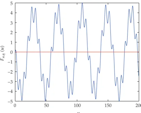
Fu Fα,ηu:sinu− m

k1

αksinηku0. 2.28

The functionFα,ηuis a non-zero, almost periodic function and has mean value 0. In fact,

Fα,ηuis quasiperiodic. ByLemma 2.3ii,Fα,ηhas infinitely many positive zeros tending to

∞. SeeFigure 1. HenceΣ0

α,ηcontains a sequence of positive eigenvalues tending to∞.

Next we consider possible negative eigenvaluesλ−u2ofM0, whereu >0. In this

case,2.24is the same as

Fu Fα,ηu:sinhu− m

k1

αksinhηku0. 2.29

See the first equality of2.26. Notice thatFuis analytic inu. Asηk∈0,1, one has

lim

u→∞ Fu

sinhu1. 2.30

Thus2.29has at most finitely many positive solutions. HenceΣ0

α,ηcontains at most finitely

many negative eigenvalues.

As both2.28and2.29have only isolated solutions, the above two cases show that all real eigenvalues ofM0can be listed as in2.27.

The quasi-periodic functionFα,ηuis as inFigure 1.

2.3. Nonexistence of Nonreal Eigenvalues

To study real eigenvalues of problem M0, the authors of 5, 6, 8 have imposed some

restrictions onα αk∈Rm. The typical conditions are

With some restrictions onα αk, we will prove thatΣ0α,ηconsists of only real eigenvalues.

It follows from the H ¨older inequality that

−5

−4

−3

−2

−1 0 1 2 3 4 5

0 50 100 150 200

Fα,η

u

u

Figure 1:FunctionFα,ηuand its positive zeros, wherem1,α4 andη1/2π.

Finally, by the H ¨older inequality, assumption2.32implies thatα ≤√m· αl2 ≤1.

For anyu∈0, π/2, the functionFα,ηuof2.28satisfies

Fα,ηu≥sinu− m

k1

|αk|sinηku

>sinu−

_m

k1 |αk|

sinu

≥0.

2.36

Hence2.28shows thatΣ0_α,η⊂π/22,∞.

Remark 2.6. Condition2.32is sharp. For example, letm1 andη1/3.Example 2.1shows thatΣ0

α,ηcontains nonreal eigenvalues ifα <−1. Similarly, by lettingm1 andη1/5, one

can verify thatΣ0_α,ηcontains nonreal eigenvalues whenα >1.

3. Structure of Eigenvalues of Non-Zero Potentials

Givenq∈L1_Rand complex parameterλ∈C, the fundamental solutions of1.1are denoted byykx, λ, q,k1,2. That is, they are solutions of1.1satisfying the initial values

y1

0, λ, qy₂0, λ, q1, y₁0, λ, qy2

0, λ, q0. 3.1

Notice thatykx, λ, qare entire functions ofλ∈C. See11. To studyMq, let us introduce

Mqλ:y2

1, λ, q−

m

k1

αky2

ηk, λ, q

which is an entire function ofλ∈C. See2.25for the caseq0. Notice thatMqλis real for

λ∈R. Thenλ∈Σqα,ηif and only if

Mqλ 0. 3.3

3.1. Basic Estimates

Lemma 3.1. Givenβ∈0,1, one has

lim

v∈R |v| →∞

|sinuiv| exp|v|

1

2, limv∈R |v| →∞

_sinβuiv

exp|v| 0 3.4

uniformly inu∈R.

Proof. Suppose thatu, v∈R. We have from2.26

|sinuiv|

sin2usinh2v∈sinh|v|,coshv,

_sinβuivsin2_βusinh2_{βv≤coshβv≤expβ|v|.}

3.5

The uniform limits in3.4are evident.

For the functionFu Fα,ηuof2.28, one has the following result on its amplitude.

Lemma 3.2. Givenα, η ∈ Rm_×Δm_{, there exist a constantc}

α,η > 0and a sequence{an}n∈Nof

increasing positive numbers such thatan↑∞and

−1n_Fa

n≥cα,η ∀n∈N. 3.6

Proof. Recall thatFuis quasi-periodic and has the mean value 0. Denote that

cα,η:

1 2max

sup

u∈R

Fu,−inf

u∈RFu

. 3.7

Thencα,η>0. The construction for{an}n∈Nis as follows. By2.15, one has somea1∈0,∞

such thatFa1≤ −cα,η. By lettingA a11 in2.16, we have somea2 ∈ a11,∞such

thatF2a2≥ cα,η. Then, by lettingA a21 in2.15, we have somea3 ∈a21,∞such

Lemma 3.3basic estimates,11, page 13, Theorem 3. Letq ∈L1_Randλ ∈ C. There hold the following estimates for allx∈0,1

y1

x, λ, q−Cλx≤

1

√λexp _Im

λxq_L1_0,x

, _3.8

y2

x, λ, q−Sλx≤

1

|λ|exp

_Im

λxq_L1_0,x

, 3.9

_y

1

x, λ, q−C_λx≤qexpImλxq_L1_0,x

, 3.10

y₂x, λ, q−S_λx≤ q

√λ

expImλxq_L1_0,x

. _3.11

Remark 3.4. For their purpose, the authors of 11 have proved 3.8–3.11 for complex potentialsq ∈ L2

C : L20,1,C. For example, in 3.8–3.11, the terms q andqL1_0,x

are replaced by qL2_0,1 and q_L2_0,1 ·√x, respectively in 11. Inspecting their proofs,

especially the proof of11, pages 7–9, Theorem 1, one can find that estimates3.8–3.11

are also true forL1_{potentialsq. Moreover, these estimates can be established even for linear}

measure differential equations with general measures16. By the H ¨older inequality, one has

qq_L1_0,1≤q_L2_0,1, q_L1_0,x≤q_L2_0,1· √

x. 3.12

This is why the authors of11have used these terms in3.8–3.11.

Lemma 3.5. There holds the following estimate forMqλ:

Mqλ−M0λ≤

Bexp|Imω|

|ω|2 , ω:

λ∈C, 3.13

where

BBα, q: 1αexpq∈1,∞. 3.14

Proof. Defineϕx:y2x, λ, q−Sλx. From3.9, we have

By2.25and3.2, we have

Mqλ−M0λ ϕ1−

m

k1

αkϕ

ηk

≤ϕ1

m

k1 |αk|ϕ

ηk

≤1αexpq|ω|−2exp|Imω|.

3.16

This gives3.13.

Lemma 3.6. One hasMqλ/≡0onR. Consequently, there existsλ0∈Rsuch thatλ0/∈Σqα,η.

Proof. Otherwise, we haveMqλ≡0 onR. Notice that

M0

u2≡ Fu

u , u >0. 3.17

Letλa2

nin3.13, where{an}n∈Nis as inLemma 3.2. We have

Fan

an

M0

a2_n≤ B a2

n

∀n∈N. 3.18

Hence limn→∞|Fan| ≤B/an → 0, a contradiction with3.6.

3.2. Eigenvalues with General Parameters

The most general results on spectrumΣqα,ηofMqare stated as inTheorem 1.1.

Proof ofTheorem 1.1. We argue as in general spectrum theory12. ByLemma 3.6, there exists λ0∈Rsuch thatλ0/∈Σqα,η. That is, the following equation:

−yqxy−λ0y0 3.19

has only the trivial solutiony 0 satisfying boundary condition1.2. LetG0x, ube the

Green function associated with problem3.19-1.2. Thenλ∈Σqα,ηif and only ifλ /λ0and

−yqx−λ0

y λ−λ0y 3.20

has nontrivial solution yx satisfying 1.2. In other words, λ ∈ Σqα,η if and only if the

following equation:

has non-trivial solutiony, where

Lqyx:

₁

0

G0x, u

qu−λ0

yudu. 3.22

SinceLqis a compact linear operator, one sees that this happens when and only when 1/λ−

λ0 ∈ σLq ⊂ C, where σLqis the spectrum of Lq. Hence Σqα,η consists of a sequence of

eigenvalues which can accumulate only at infinity ofC. Forλ∈C, denote that

λω2, ωλuiv, u, v∈R. 3.23

Suppose thatλ∈Σqα,ηandλ /0. ThenMqλ 0 and3.13implies that

Bexp|v|

|ω|2 ≥

_{Mqλ−M0λ|M0λ|}

sinω− m

k1αksinηkω

ω

≥ |sinuiv| − m

k1|αk|sinηkuiv

|ω| .

3.24

We conclude that all non-zero eigenvaluesλ∈Σqα,ηsatisfy

|ω| ·|sinuiv| −

m

k1|αk|sinηkuiv

exp|v| ≤B. 3.25

Let us derive some consequences from estimate3.25forλ∈Σqα,η.

iSince|ω| ≥ |v|, it follows from the uniform limits in3.4that

lim

|v||Imω| →∞|ω| ·

|sinuiv| −m_k1|αk|sinηkuiv

exp|v| ∞. 3.26

Thus there exists somehhα,η,q>0 such that

λ∈Σqα,η⇒ω

λ∈Hh:{ω∈C:|Imω|< h}. 3.27

The horizontal stripHh of 3.27in the ω-plane is transformed by 3.23to the following

half-planePrin theλ-plane:

Σq

iiLetr > −h2_{. We assert that}

Σqα,η∩ {λ∈C: Re λ≤r} Σ q α,η∩

λ∈C:−h2< Re λ≤r 3.29

contains at most finitely many eigenvalues. Otherwise, suppose that

Σq α,η∩

λ∈C:−h2< Re λ≤r 3.30

contains infinitely many λn, n ∈ N. Since 3.3 has only isolated solutions, we have

necessarily|Imλn| → ∞. By denoting

λnunivn, one has

−h2< u2_n−v_n2≤r, 2|un||vn| −→∞. 3.31

In particular,|vn| → ∞. Now estimate3.25reads as

|sinunivn|

exp|vn| ≤

_m

k1|αk|sinηkunivn

exp|vn|

o1 asn−→ ∞. 3.32

This is impossible because we have the uniform limits3.4.

Combiningiandii, we know thatΣqα,ηcan be listed as in1.6.

Though problem Mq is not symmetric, Σqα,η always contains infinitely many real

eigenvalues, as stated inTheorem 1.2.

Proof ofTheorem 1.2. We need to only consider positive eigenvalues ofMq. Let λ a2n in

3.13, where{an}n∈Nis as inLemma 3.2. By using3.17, we have

Mq

a2_n−Fan an

≤ B

a2n

∀n∈N. 3.33

Sincean↑∞, w.l.o.g., we can assume thatan≥2B/cα,ηfor alln∈N. Thus

anMq

a2_n−Fan≤ B

an ≤

cα,η

2 ∀n∈N. 3.34

By using3.6, we conclude that

−1n_M q

a2_n>0 ∀n∈N. 3.35

Hence3.3has at least one positive solutionλnin each intervala2n, a2n1,n∈N. Combining

withTheorem 1.1,Σqα,η∩Rconsists of a sequence of real eigenvalues tending to∞. Hence

Σq

4. Nonexistence of Nonreal Eigenvalues for Small

α

We will apply the Rouch´e theorem to give further results onΣqα,ηwhenαis small, following

the approach in11for the Dirichlet problem1.1-1.4, which corresponds to Mqwith

α0. Let us recall the Rouch´e theorem.

Lemma 4.1Rouch´e theorem. Suppose thatfz, gzare entire functions ofz∈C. If|gz|<

|fz|on a Jordan curveC, thenfzandfzgzhave the same number of zeros insideC, counted multiplicities.

For later use, let us introduce the following elementary function:

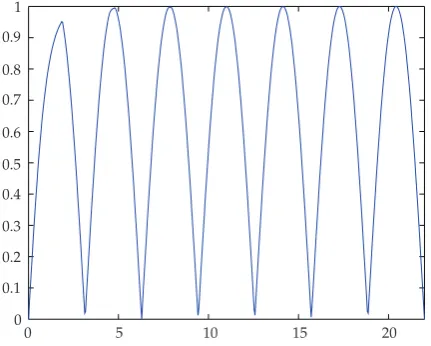
Gω:

sin2usinh2v

coshv

1−

cosu coshv

2

, ωuiv∈C. 4.1

ThenGω≡Gωπ. Obviously,Gω 0 if and only ifωnπ,n∈Z. Define

Gr: min

ω∈Cr

Gω∈0,1, r ∈0,∞, _4.2

whereCris the circle in theω-plane

Cr:{ωuiv∈C:|ω|r}. 4.3

ThenGnπ 0,n∈Z :{0,1, . . . , n, . . .}, and 0< Gr<1 for allr ∈0,∞\πZ. Letr0be the unique solution of the following equation:

tanhrsinr, r∈0, π. 4.4

Numerically, r0 . 1.8751 . 0.5968π. The following facts can be verified by elementary

arguments.

Lemma 4.2. One has

Gr

⎧ ⎨ ⎩

tanhr forr∈0,r0,

sin r forr∈r0, π,

lim

n→∞G

n1

2 π 1.

4.5

0 0.1 0.2 0.3 0.4 0.5 0.6 0.7 0.8 0.9 1

0 5 10 15 20

Figure 2:The functionGr, wherer∈0,7π.

r0

nπ n1π

0

h0

Figure 3:Finding zeros ofMqω2in theω-plane.

4.1. Large Eigenvalues

In the following we apply the Rouch´e theorem to study the spectrumΣqα,η, that is, the zeros of

the functionMqλin theλ-plane. To this end, we consider problemMqas a perturbation

of the Dirichlet problemD0, whose eigenvalues are zeros of the function

D0λ:

sin√λ

√

λ , λ∈C. 4.6

Letλω2_{. Equation3.3is the same as}

D0

ω2_M

q

ω2_−D 0

which is considered as a perturbation of the following equation:

D0

ω2 sinω

ω 0, ω∈C. 4.8

Due to the form of4.7and4.8, one needs to only consider solutions in the right half-plane

Cofω. Notice that all solutions of4.8arenπ,n∈N, which are simple zeros ofD0ω2. For

anyα /0, we do not know whether all zeros of4.7are real. In order to overcome this, the proof is complicated than that in11.

Let us derive another consequence from estimate3.25with some restriction onα αk. Suppose thatα∈Rmsatisfiesα<1. Define the positive function

Wh Wh;α, qdef Bexph

sinhh− αcoshh, h∈arctanhα,∞, 4.9

whereBBα, qis as in3.14. ThenWhis decreasing inh∈arctanhα,∞.

Lemma 4.3. Suppose that

α<1, h > arctanhα. 4.10

Then for anyλω2∈Σqα,η, whereη∈Δm, one has

either|Imω|< h, or |ω| ≤Wh. 4.11

Proof. We keep the notations in3.23Letλ ω2 ∈Σqα,η. If|v||Imω| ≥ h, it follows from

2.26and3.25that

Bexp|v|

|ω| ≥ |sinuiv| −

m

k1

|αk|sinηkuiv

sin2usinh2v−

m

k1 |αk|

sin2ηkusinh2ηkv

≥sinh|v| −

m

k1 |αk|

1sinh2v

sinh|v| − αcoshv.

4.12

Using the functionW·in4.9, we obtain|ω| ≤W|v|≤Wh. This proves4.11.

Consider the following circles of theω-plane:

Lemma 4.4. Letn, rbe as in4.13. one has

Proof ofTheorem 1.3. Let

where the constantr0 ∈π/2, πis as inLemma 4.2. One has sinr0 . 0.9541 and tanhh0 .

0.7714. Denote byDn,r0the disc enclosed by the circleCn,r0, that is,

Dn,r0 :{ω∈C:|ω−nπ|<r0}, n∈Z. 4.21

Sincer0> π/2,Dn,r0intersectsDn1,r0. SeeFigure 3.

In the following, we always assume thatα∈Rm_satisfies

α ≤ 1

2 <minsin r0,tanhh0. 4.22

Suggested by3.14,4.9, and4.11, we denote

c0def 1

1/2exph0

sinhh0−1/2coshh0

3 exph0

2 sinhh0−coshh0

.

9.7873. 4.23

Then, for allαas in4.22, by4.9one has

Wh0;α, q

1αexph0

sinhh0− αcoshh0 exp

_{q≤c0expq. 4.24}

Suppose that

λ0ω20 ∈Σ

q

α,η, |ω0| ≥11 expq. 4.25

Let us show that λ0 must be positive. In fact, 4.25 implies that |ω0| ≥ 11 expq >

Wh0;α, q. By result4.11, we have|Im ω0| < h0. Hence ω0 is a zero of Mqω2 inside

some discDn,r0. SeeFigure 3. W.l.o.g., let us assume thatn >0. Thennsatisfies

nπ≥ |ω0| − |ω0−nπ|>11 expq−r0. 4.26

For anyω∈Cn,r0, one has

It follows from4.5thatGr0 sinhr0sinr0. By4.14, we have the estimate

uniqueness, all eigenvaluesλ0as in4.25must be positive.

Finally, it follows fromTheorem 1.1thatΣqα,ηcontains at most finitely manyλwhich

do not satisfy4.25. Thus the proof ofTheorem 1.3is completed.

4.2. Small Eigenvalues

Proof ofTheorem 1.4. By4.4, we can fix somennq∈Nsuch that

n≥ 11 expq π −

1

2, 4.32

1 Gn1/2π

1 2

3 expq n1/2π

<1. 4.33

Denote that

rrq:

n1

2 π

2

, DDq:{λ∈C:|λ|<r}. 4.34

In the following we assume thatα ∈Rm_{satisfies4.22, that is,α ≤ 1/2. From the}

proof ofTheorem 1.3,Σqα,η∩C\Dconsists of positive eigenvalues. See conditions4.25and

4.32. Moreover, forλ∈ ∂D, that is,|√λ| n1/2π, we obtain from estimate4.14and condition4.33that

Mqλ−D0λ

D0λ ≤

1 Gn1/2π

α 21αexpq n1/2π

≤ 1

Gn1/2π

1 2

3 expq n1/2π

<1.

4.35

Notice that equation

D0λ

sin√λ

√

λ 0, λ∈D, 4.36

hassimplesolutionsλ nπ2,n 1, . . . ,n. By the Rouch´e theorem, we conclude that, if

α ≤1/2, the following problem:

Mqλ, α 0, λ∈D, 4.37

has preciselynsolutions, counted multiplicity. HereMqλhas been written asMqλ, αto

emphasize the dependence onα.

Suppose thatα 0. Equation4.37corresponds to the Dirichlet eigenvalue problem 1.1–1.4, which has only real eigenvalues. Moreover, all solutions of4.37are simple in this case11. Hence solutions of problem4.37can be denoted byλμn, 1≤n≤n, where

−r< μ1 <· · ·< μn <r. 4.38

In the following, we apply the implicit function theorem to prove that solutions of

Sinceμn is a Dirichlet eigenvalue of problem1.1, we havebn 0. Moreover, the Liouville

theorem for1.1implies that

1det

Now the implicit function theorem is applicable to4.37. In conclusion, there exist some

constantAAq,η>0 and a continuously differentiable real-valued functionsλnαofαsuch

that

λn0 μn, Mqλnα, α≡0, α ≤Aq,η, 1≤n≤n. 4.44

Due to4.38–4.44and the continuity ofλnα, one can assume that

−r< λ1α<· · · < λnα<r ∀ α ≤Aq,η. 4.45

Thus{λnα}1≤n≤nare different eigenvalues ofMqlocated in the interval−r,r. Since4.37

Notice that the constant Aq,η in 4.44 is constructed from the implicit function

theorem. Generally speaking,Aq,ηdepends onη∈0,1and all information of the potential

q ∈ L1

R. However, during the application of the implicit function theorem to 4.37, the derivatives of∂αλnαcan be well controlled using estimates in11, like3.8–3.11. It is

possible to choose someAq,η such that it depends on the normq only. We will not give

the detailed construction. Note that this has been already observed for large eigenvalues. For example,nandrdepend only on the normqofq.

We end the paper with an open problem. Givenα, η∈Rm_×Δm_{, for anyq∈L}1

R, due toTheorem 1.2, problemMqhas always a sequence of real eigenvaluesλnq λn,α,ηq

which tends to∞. In applications of eigenvalues to nonlinear problems, the smallestreal eigenvaluesλ1qare of great importance. The main reason is that solutions of problem1.1–

1.2are oscillatory only when λ > λ1q. As for the smallest eigenvalue of the Dirichlet

problem1.1–1.4, denoted byλ1q, one has the following variational characterization:

λ1

q inf

y∈H1 00,1, y /0

1 0

y2qxy2_{dx 1}

0y2dx

. 4.46

An open problem is what is the characterization like4.46for the smallest eigenvalueλ1q

ofMq. Once this is clear, some results on nonlinear problems in5,6,8can be extended by

using eigenvalues ofMq.

Finally, let us remark that the approaches in this paper also can be applied to other multi-point boundary conditions like

y0 0, y1−

m

k1

αky

ηk

0 4.47

or to more general Stieltjes boundary conditions17. In this sense, eigenvalue theory can be

established for these nonsymmetric problems.

Acknowledgments

The third author is supported by the Major State Basic Research Development Program973 Programof Chinano. 2006CB805903, the Doctoral Fund of Ministry of Education of China no. 20090002110079, the Program of Introducing Talents of Discipline to Universities111 Programof Ministry of Education and State Administration of Foreign Experts Affairs of China 2007, and the National Natural Science Foundation of China no. 10531010. The authors would like to express their thanks to Ping Yan for her help during the preparation of the paper.

References

2 R. P. Agarwal and I. Kiguradze, “On multi-point boundary value problems for linear ordinary differential equations with singularities,”Journal of Mathematical Analysis and Applications, vol. 297, no. 1, pp. 131–151, 2004.

3 C. P. Gupta, S. K. Ntouyas, and P. Ch. Tsamatos, “On anm-point boundary-value problem for second-order ordinary differential equations,”Nonlinear Analysis: Theory, Methods & Applications, vol. 23, no. 11, pp. 1427–1436, 1994.

4 B. Liu and J. Yu, “Solvability of multi-point boundary value problems at resonance. I,”Indian Journal of Pure and Applied Mathematics, vol. 33, no. 4, pp. 475–494, 2002.

5 R. Ma, “Nodal solutions for a second-order m-point boundary value problem,” Czechoslovak Mathematical Journal, vol. 56131, no. 4, pp. 1243–1263, 2006.

6 R. Ma and D. O’Regan, “Nodal solutions for second-orderm-point boundary value problems with nonlinearities across several eigenvalues,”Nonlinear Analysis: Theory, Methods & Applications, vol. 64, no. 7, pp. 1562–1577, 2006.

7 F. Meng and Z. Du, “Solvability of a second-order multi-point boundary value problem at resonance,”

Applied Mathematics and Computation, vol. 208, no. 1, pp. 23–30, 2009.

8 B. P. Rynne, “Spectral properties and nodal solutions for second-order, m-point, boundary value problems,”Nonlinear Analysis: Theory, Methods & Applications, vol. 67, no. 12, pp. 3318–3327, 2007. 9 B. P. Rynne, “Second-order, three-point boundary value problems with jumping non-linearities,”

Nonlinear Analysis: Theory, Methods & Applications, vol. 68, no. 11, pp. 3294–3306, 2008.

10 M. Zhang and Y. Han, “On the applications of Leray-Schauder continuation theorem to boundary value problems of semilinear differential equations,”Annals of Differential Equations, vol. 13, no. 2, pp. 189–207, 1997.

11 J. P ¨oschel and E. Trubowitz,The Inverse Spectrum Theory, Academic Press, New York, NY, USA, 1987. 12 A. Zettl, Sturm-Liouville Theory, vol. 121 of Mathematical Surveys and Monographs, American

Mathematical Society, Providence, RI, USA, 2005.

13 B. P. Rynne, “Spectral properties of second-order, multi-point, p-Laplacian boundary value problems,”Nonlinear Analysis: Theory, Methods & Applications, vol. 72, no. 11, pp. 4244–4253, 2010. 14 A. M. Fink,Almost Periodic Differential Equations, Lecture Notes in Mathematics, Vol. 377, Springer,

Berlin, Germany, 1974.

15 J. K. Hale,Ordinary Differential Equations, John Wiley & Sons, New York, NY, USA, 2nd edition, 1969. 16 G. Meng,Continuity of solutions and eigenvalues in measures with weak∗ topology, Ph.D. dissertation,

Tsinghua University, Beijing, China, 2009.