Not Just Another Trait: Methods for the Genetic Analysis of Gene Expression

(1)

ABSTRACT

AYLOR, DAVID LAWRENCE. Not Just Another Trait: Methods for the Genetic Analysis of Gene Expression. (Under the direction of Zhao-Bang Zeng.)

Gene expression refers to the process by which DNA is transcribed to mRNA. It is

now possible to measure genome-wide transcript abundance in many genetically distinct individuals. Genetical genomics refers to the application of quantitative genetic techniques

to such data. We present two analyses of gene expression in distinct experimental populations.

We first present a method for a classical epistasis analysis that includes gene

expression measurements. We propose a framework for estimating and interpreting epistasis

that borrows from both classical and quantitative approaches. Regression analysis estimates the effects of gene deletions as well as interactions and significant effects are selected such

that a reduced model describes each expression trait. We then show how the resulting models correspond to specific hierarchical relationships between two regulator genes and a target gene. These hierarchical relationships are the building blocks of systems diagrams and

genetic pathways. Our framework can serve as a foundation for future epistasis analyses based on genomic data.

Secondly, we analyze expression quantitative trait locus mapping (eQTL) results in a segregating yeast population. We use prior information about yeast pathways to group expression measurements and ask questions about pathway regulation. We find that while

(2)

propose a possible explanation for our observations and describe how they fit in with previous interpretations of these data.

Lastly, we present a tool for manipulating sequence data within a population. Our

software enables the user to pull out important features from a multiple alignment such as variable sites, unique haplotypes, and insertions or deletions. The output is compatible with

(3)

Not Just Another Trait: Methods for the Genetic Analysis of Gene Expression

by

David Lawrence Aylor

A dissertation submitted to the Graduate Faculty of North Carolina State University

in partial fulfillment of the requirements for the Degree of

Doctor of Philosophy

Bioinformatics

Raleigh, NC 2008

APPROVED BY:

__________________________ ________________________ Dr. Zhao-Bang Zeng Dr. Ignazio Carbone

Committee Chair

_________________________ _________________________ Dr. Jeffrey Thorne Dr. Philip Awadalla

(4)

Dedication

(5)

Biography

David Lawrence Aylor was born in Woodbridge, VA, about thirty miles south of Washington, D.C. His parents, Mrs. Bonita Satterfield Aylor and the late Mr. Herman Henry

Aylor, Jr. raised their only son with an emphasis on family. Every Sunday after church they spent the afternoon at his grandmother’s house with aunts, uncles and cousins. His favorite

pastime was drawing, though most free time was spent outdoors.

It is a point of pride that David attended public schools throughout his academic career, from kindergarten to graduate school. At the University of Virginia, he received his

Bachelors of Arts in Environmental Sciences in 1996. Summer courses at Mountain Lake Biological Station the year before were his first exposure to academic biology and were

influential, yet he was eager to see the world and would not pursue additional formal education for another six years.

The last half of his graduation year and the first months of the next were spent in

Anchorage, AK as an intern for The Nature Conservancy. His task was to develop maps of wildlife habitat using geographic information systems, a harbinger of the computing and

biology combination yet to come. Computing would take the lead for the next five years, which were spent as a software developer in Charleston, SC and New York, NY. Media coverage of the genome projects led to new enthusiasm for computational biology and

(6)

List of Tables

Table 2.1. Correspondence between regression models

and biological models ... 36 Table 3.1 Putative Pathway Regulator QTL... 75

Table 4.1 File formats currently generated using

(8)

List of Figures

Figure 2.1 Modeling the relationship A is an upstream repressor of B ... 34 Figure 2.2 Post-aggregation distributions of best-fit models

at p < 0.01 significance thresholds ... 41

Figure 2.3 Modeling the relationship A is an upstream repressor of B,

which represses a target gene ... 53

Figure 2.4 Modeling the relationship A is an upstream enhancer of B,

which represses a target gene ... 54

Figure 2.5 Modeling the relationship A is an upstream enhancer of B,

which enhances a target gene ... 55

Figure 2.6 Distribution of best-fit models pre-aggregation... 56 Figure 2.7 Distribution of best-fit models post-aggregation (untransformed data)... 57

Figure 2.8 Distribution of best-fit models at varying significance

thresholds pre-aggregation... 58

Figure 2.9 Distribution of best-fit models at varying significance

thresholds post-aggregation ... 59

(9)

Chapter 1

(10)

Quantitative Genetics Concepts and Data

From the time of Mendel until the characterization of the genetic code, genes were physically unobserved. Mendel observed that offspring inherit traits from their parents in

discrete units, and the term gene was later coined to describe this functional unit of heredity. Alleles are functionally distinct forms of a particular gene. Some traits vary continuously

rather than discretely and at first did not appear to be inherited according to Mendel’s rules. These traits were termed quantitative, meaning that they can be measured; they traits are also referred to as complex traits. Quantitative genetics is the study of such traits (Lynch and

Walsh 1998). R.A. Fisher (1918) showed how combinations of multiple genes could explain quantitative variation in a population, and this has been a fundamental assumption of most

subsequent quantitative genetic models. Non-genetic effects such as those imposed by different environments can also affect quantitative traits.

Two types of data are required for quantitative genetic analyses. These are the

phenotypic variation and the genetic structure of the study population. Phenotypic variation

or trait values can be measured in a variety of ways depending on the continuous trait being

investigated. The degree of relatedness is usually a product of experimental design. Such

analyses estimate such quantities as the proportion of heritable variation in a trait and its

potential response to selection. These estimates are statistical in nature and describe the

population of study organisms rather than any one individual. The methods used are

predominately regression-based and rely on several assumptions about the properties of

(11)

are additive and should be modeled as such. Deviations from additivity are interpreted as

interactions between genes. Dominance refers to interactions between alleles within a locus.

Epistasis refers to interactions between alleles at separate loci. Some models are extended to

include such interaction effects.

Linkage analysis refers to a body of methods based on the observation that alleles do

not always segregate independently. If two traits are observed together in offspring often but

not always, then the allele combinations not observed in the parents are called recombinants,

and recombination frequency is the fraction of these offspring. This concept was extended to

create the first genetic map in fruit flies (Sturtevant 1919). To construct a linkage map, one

must assume that genes exhibiting low frequency of recombination are located closer to each

other on the chromosome, which had recently been validated as vectors of heredity (Morgan

1910). These frequencies are the genetic distance upon which the map is based. In

eukaryotes, recombination is now known to be due to the biological phenomenon of crossing

over during meiosis. It is notable that the original markers were phenotypes of mutants, and

linkage maps predated many of the concepts we now associate with them.

The physical material of genes was unknown until the 1950s, when the structure of the DNA molecule was discovered and the gene concept expanded to describe something both functional and physical. A gene in this sense is a molecular region that is a template for an

mRNA transcript. In the intervening years, the field of molecular genetics has provided details about how genes are transcribed into mRNA that is subsequently translated into

(12)

Molecular Markers and QTL Mapping

Polymorphisms are individual differences in the DNA molecules within a population.

In modern genetics, observed polymorphisms are called molecular markers and can be used to

create linkage maps. Various types of markers exist including microsatellites, Restriction

Fragment Length Polymorphisms (RFLPs), and Single Nucleotide Polymorphisms (SNPs).

These are often associated with a particular technology for detecting variation.

Quantitative Trait Locus (QTL) mapping takes advantage of the gene’s dual nature, by associating variation in observed traits with molecular markers. In short, the functional

gene is mapped to a physical location. The goal of QTL mapping is to locate the physical

regions of an organism’s DNA that are linked to the trait of interest. Regions that are linked

to a particular trait are called quantitative trait loci (QTLs). QTL mapping begins with

observed trait measurements, a study population with a known degree of relatedness, and

molecular markers from each individual in the study population. The relationship between

individuals in the mapping population is usually a product of the experimental design. The

molecular marker data should be sufficient to create a linkage map; it is common to have

between a few dozen to a few hundred genetic markers spread throughout the genome of the

study population. As mapping populations undergo more generations of recombination, they

require more markers to study. This generally translates to increased resolution but less

(13)

The simplest method of associating markers with trait values is the single marker

analysis (SMA). For each marker, individuals are separated into two groups based on their

marker allele and we test if the trait mean is different between the groups. The weaknesses of

this approach are that it cannot identify multiple QTLs, cannot estimate QTL position,

underestimates the QTL effect, and is not very powerful (Zeng 2000). A vast body of

literature outlines more sophisticated methods for mapping the location of QTLs and the

magnitude of their effect.

Interval mapping (IM) (Lander and Botstein 1989) extends the simple SMA test by

testing association with the regions between two markers. This method is notable because it

accounts for recombination between the markers and the QTL. The QTL is assumed to be

located somewhere in the interval and at some genetic distance from each marker. A

likelihood ratio (LR) test is used for each interval along the linkage map, and relates the

hypothesis that a QTL in the given interval has an effect on the trait versus the hypothesis

that it does not. The LR test statistic is usually reported as a log of odds (LOD) score, which

is the same value arbitrarily scaled differently and historically used in human genetics.

Composite Interval Mapping (CIM) allows multiple QTLs to be evaluated in the same

genetic model (Zeng 1993; Zeng 1994). This more closely agrees with the theory of

quantitative traits, in which many genes combine to determine trait values. Multiple QTL

models are accomplished in a sequential manner by first adding one QTL to the model in the

(14)

Interval Mapping (MIM) (Kao et al 1999; Zeng et al 1999) refines CIM by virtue of an

improved search procedure and allowance of more complex genetic models. The need for a

QTL significance threshold is common to all these methods. This is an area of current

development due to the computational burden of permutation testing, which has been the

most successful approach (Churchill and Doerge 1994; Doerge and Churchill 1996).

Each QTL is assumed to contain one or more individual genes that contribute to the

observed phenotype. However, QTL mapping is limited in resolution by the size of the

mapping population, the amount of recombination in the population, and the density and

distribution of markers. For these reasons, relatively few causative genes have been identified

despite thousands of QTLs found for myriad traits. Generally, additional data must be

incorporated to fine-map QTLs. However, following up on QTL results with additional

genetic data is increasingly feasible because of advances in sequencing technology and the

subsequent lower costs.

QTL mapping revolutionized genetic data analysis during an era in which phenotypic

data was plentiful and genetic markers increased in availability. In model organisms, QTL

mapping has led to discovery of new genes linked to well-studied phenotypes. It has allowed

for advances in plant and animal breeding through identification of regions linked to traits of

interest and marker-assisted selection. Most importantly, QTL mapping has provided new

insights into the architecture of quantitative traits such as the distribution of QTL effects, the

(15)

The Genomic Era and Expression QTL Mapping

Again, advances in molecular biology are pushing the cutting edge of quantitative

genetics. A genome is the entirety of the unique DNA belonging to a particular species, and

the 1990s saw a flurry of genome projects for a variety of species. The goal of these projects

is to create a physical map that contains the nucleotide sequence of an entire genome. Genes and other features are all placed on the map by processes referred to collectively as genome

annotation. Some genes are located because they physically “look like” other genes. Others genes are mapped to specific functions through experimental means. Much of the progress in annotation was due to new technologies that allowed many simultaneous measurements. A

litany of words ending in “omics” describes methods for measuring many molecules simultaneously – be they cellular proteins, metabolites, or mRNA transcripts. Gene

expression refers to the relative amount of mRNA transcript produced by a particular gene, and the number of these experiments skyrocketed since the advent of cDNA microarrays and

later manufactured oligonucleotide arrays for model organisms. These high throughput

technologies have steadily grown in popularity, improved in quality, and lessened in cost

over the past decade. During this time, procuring traditional phenotype data has not

translated well to high-throughput methods and is relatively costly and time-consuming.

As gathering genomic data for segregating populations has become feasible, these data

have been considered as continuous traits and candidates for QTL mapping in what has been

(16)

substitutes gene expression measurements for phenotype and uses essentially the same

methods as traditional QTL mapping. However, rather than considering one or a few classical

traits, many or even thousands of expression traits (e-traits) are considered. In practice,

eQTL mapping is generally performed by iteratively applying traditional QTL mapping

techniques to each individual expression measurement.

Expression traits have several appealing properties. Foremost, a physical location is

associated with each trait, and one can distinguish between proximate cis-QTLs and

trans-QTLs that locate elsewhere in the genome. Cis-trans-QTLs indicate variation located in the same

physical location as the gene itself. This may reflect variation in promoters or allelic

variation. QTLs that regulate traits that are not collocated are called trans-QTL. Trans-

regulatory polymorphisms may reside in regulatory proteins such as transcription factors, be

indirect effects from genes upstream in regulatory pathways (Brem et al. 2002), or represent

other mechanisms of regulatory feedback. Two patterns have been apparent in all eQTL

studies to date. The first is a significant group of e-traits linked to a cis-QTL. The second

pattern is multiple trans-QTLs that are shared by many traits, sometimes called hotspots.

These two features have become starting points for how we describe expression QTL results

and are central to how we interpret them.

Additionally, it is an important difference from phenotypic measurements that expression

traits have an intrinsic molecular biological role (Schadt et al. 2003). Bioinformatics databases

(17)

associated with phenotypes and molecular biological functions without any additional

experimentation. Likewise, e-traits can be grouped according to such data. This additional

information can generate hypotheses regarding the gene underlying QTL.

Three Intergenic Relationships in Expression QTL Experiments

Traditional QTL mapping reflects a relationship between a physical region and a

phenotype. Inasmuch as we assume a causative gene underlies the QTL, this can be

considered a gene-trait relationship. Since in eQTL mapping the trait is itself a gene, the

trans-QTL is a relationship between two genes. A polymorphism in one gene affects the

expression of another. Epistasis can be modeled just as in traditional QTL mapping, as part

of the genetic model. Based on the same assumption that a gene underlies each QTL, this is

also a relationship between genes. Polymorphisms in two genes affect the expression of a

third, or one of the genes themselves if one of the QTL is in cis-. Lastly, there are

relationships between the expression measurements that represent a third relationship

between genes. Expression traits can be correlated expression of genes), share a QTL

(co-regulation of genes), or represent genes of shared function. These three relationships allow us

to interpret eQTL results in the context of regulatory networks. Depending on the

experiment, additional relationships between genes and phenotype can also be explored.

We present several lines of research from the past five years in this context.

(18)

genetic variation. Mice studies showed system level genetics in the context of different

organs, and the community has made unique contributions to exploring the relationships

between expression traits. Plant research has contributed the most in terms of integrating

expression QTL mapping with phenotype and other biomolecular data.

Expression QTL in Yeast

In a series of papers, Leonid Kruglyak and colleagues presented expression QTL mapping results from yeast (Brem and Kruglyak 2005; Brem et al. 2005; Brem et al. 2002; Yvert et al. 2003). A wild isolate from a vineyard was crossed with a standard laboratory

strain, and expression was measured on 112 haploid segregants. Yeast have a haploid phase in their life cycle, so these segregants are genetically comparable to a diploid F1. Both

capture one generation of recombination. Preliminary results were released based on 40 segregants and later 86 segregants. Gene expression was measured for 6216 trait genes; 489 were eventually disregarded due to an independent survey of the yeast genome (Kellis et al.

2003), leaving 5727 genes. In a controlled environment, one quarter of the expression traits measured were differentially expressed between the parent strains at P < 0.005. They

estimated a median heritability of 0.84 using mid-parent/offspring regression. Because there is no dominance in haploid organisms, this is heritability in both the broad and narrow sense. 3312 genetic markers were typed.

(19)

cis-Eight shared trans-regulators accounted for over 40% of QTL, and each was characterized as being enriched for genes of a common function. For the shared regulators that also have a cis- linkage, the trait with the cis- linkage was inferred to be the gene harboring a causative

polymorphism. Candidate regulator genes were supposed by prior knowledge of genes in the linkage region, but for which the corresponding expression trait had no cis-QTL.

In a follow-up paper, Yvert et al (Yvert et al. 2003) found many additional linkages

using 86 segregants (2294 at P < 3.4 × 10-5, 992 at P < 5 × 10-7). The number of shared trans-regulators grew to thirteen. In this report they used correlation-based k-means

clustering to group similar traits based on their expression profiles. Thirty percent of

expression traits clustered with at least one other gene. They found 593 clusters of at least two genes and 205 larger clusters. This grouping approach is independent of the linkage

analysis, but groups based solely on data generated from the experimental cross. These clusters were enriched for genes with shared annotations, and the mean expression of genes within each cluster linked to genetic variation for over half of clusters. They found that

trans-QTLs regulating clusters were rarely transcription factors and noted diverse biological

functions among putative trans-regulator genes. This may be due to strong evolutionary

conservation among transcription factors.

With additional samples (Brem and Kruglyak 2005), they estimated slightly more

expression traits with at least one QTL (2984 at FDR = 0.05). Most of these traits had high

heritability of over 0.69. They explored the number of loci underlying these high heritability

(20)

There was a direct relationship between increasing model complexity and the proportion of

traits supporting each model, suggesting that expression traits are regulated by many QTL.

The additional information associated with expression traits can be used to identify the

candidate genes underlying QTL. These methods have perhaps been developed best in yeast

due to the wealth of biological information available on its molecular biology. Prior

knowledge regarding the function of the genes in a QTL region has in several cases provided a

clear candidate for positional cloning and functional assays. However, it is not feasible to

conduct additional experiments for more than a few QTL. Computational approaches

combine experimental data with bioinformatics. Bing and Hoeschle (2005) correlated the

expression profiles of genes located in each QTL region with the expression profile of traits

linked to that QTL. This approach assumes that related genes have strong correlations in

their expression. It also indirectly assumes that the causative gene has a cis-QTL, since the

marker would necessarily be correlated with both expression profiles if they were correlated

with each other. However, they identified candidate genes for both cis- and trans-QTL,

suggesting for the trans-QTLs that the underlying cis- regulation did not meet the significance

threshold needed to declare a QTL in the linkage analysis.

Epistasis: Results from Yeast

The same yeast cross has also led to insights in the second intergenic relationship --

(21)

Modeling epistasis in a segregating population involves statistically testing for interaction

between each pair of loci or putative QTL. Testing all possible pair of loci is

computationally demanding and has low power because of the enormous number of tests that

must be performed. Epistasis is not always included in traditional QTL models, but such

issues are compounded when thousands of expression traits are analyzed. Brem et al (2005)

used a two-stage search strategy to find secondary loci only after conditioning on a primary

locus, and then fitting a model including effects for both loci and an interaction. They found

65% of expression traits showed significant epistasis at P < 0.05. Creating yeast strains with

each of the four allelic combinations validated a significant interaction between MAT and

GPA1 loci. The ability to manipulate yeast so easily makes them ideal for epistasis analyses

at a range of genetic variation. Zou and Zeng applied Multiple Interval Mapping to the same

data set, which also searches for models including epistasis (Zou and Zeng 2008).

Expression QTL in Mice

Schadt and colleagues showed that similar approaches could be used in mice (Schadt et al.

2003). They profiled 111 F2 mice from a cross of standard laboratory strains (C5BL/6J ×

DBA2J). They measured gene expression in liver cells because of the liver’s role in obesity,

which was their target phenotype. Using interval mapping, they observed that cis-QTLs

were generally of larger effect than trans-QTLs, and found QTL associated with the major

(22)

with phenotype by measuring fat pad mass on the mice. The expression data allowed them

to identify two distinct expression profiles among the high fat mice, suggesting disease

subtypes controlled by unique QTLs.

Two concurrently released papers extended this approach using the BXD recombinant

inbred (RI) strains (Bystrykh et al. 2005; Chesler et al. 2005) to profile expression QTLs in

two tissues. Using a 10% FDR they found that 83 of 88 QTLs were cis- in the brain. This

is consistent with cis-QTLs having larger effects sizes than trans-QTLs; the more

conservative the significance threshold is, the higher the ratio of cis- to trans- should be.

Hotspots were prevalent but did not collocate between these three experiments, meaning that

genetic control of transcription is tissue specific.

Relationships Between Expression Traits

It is intuitive to group expression traits that share a QTL and ask whether those traits

may be related biologically. Another approach is to group related traits before the mapping

analysis. Several methods have been explored that fall into two general types. The first type

groups traits based on expression measurements from the experimental data. Clustering traits

by expression profiles is a simple method that has been prevalent in the literature.

Alternately, sets of genes can be defined a priori. Kliebenstein et al (Kliebenstein et al. 2006)

(23)

published studies or cumulative experimental results. We present an a priori analysis for

yeast in Chapter 3.

Composite trait mapping has been used in a variety of organisms (Ghazalpour et al. 2006; Kliebenstein et al. 2006; Yvert et al. 2003). This refers to mapping a trait derived from averaging or otherwise combining multiple grouped expression traits. In yeast and mice, the

expression trait values within each cluster were averaged for every individual, and this average was treated as that individual’s trait value for linkage analysis. In yeast, 304 of 593

clusters showed some linkage at P < 3.4 × 10-5. The idea behind composite traits mapping is to increase the power to identify shared regulators. However, shared regulators may not be present for every group and this could lead to incorrect conclusions.

A method for composite trait mapping is illustrated clearly in mice (Ghazalpour et al.

2006). They propose a four-step process in which traits are related by constructing a gene co-expression network, the biological significance of each module is determined from

referencing bioinformatics data, a composite (average) trait is mapped to QTLs, and the relationship between QTL and module is reevaluated for biological relevance. They group traits based on pair-wise correlation of expression values, and refer to such groups as

network modules. The biological significance of each module is determined by enrichment for Gene Ontology (GO) terms or pathways from the Kyoto Encyclopedia of Genes and

Genomes (KEGG). QTLs linked to the composite trait for a given module are called module QTLs (mQTLs). Markers within each mQTL region were evaluated based on correlation with each trait within the module. This framework captures the essentials of most composite

(24)

Expression QTL in Plants

A recent study in Arabidopsis captures variation from 211 recombinant inbred lines (RIL)

(West et al. 2007). Sixty-nine percent of 22,746 e-traits linked to QTLs at a P < 0.05

significance threshold. One third of these had a cis-QTL, which is slightly more than in

yeast. One explanation for this is more variation was captured in the parental generation. In

general, patterns in plants match those in other eukaryotes, including the relative proportion

of cis- and trans- and the presence of hotspots.

While the techniques of eQTL mapping vary little between organisms, the plants

community has contributed the most in terms of integrating the many levels of biomolecular

variation including markers, expression, metabolites, and phenotypes. Jansen and Nap

(2001) envisioned such an approach when they conceived genetical genomics and mentioned

it explicitly. However, such data remain rare because of their complexity and expense. When

gene expression correlates with a complex phenotype, the corresponding expression traits

may reflect the molecular basis of that phenotype at a level intermediate between genotype

and phenotype. The presumption is that expression QTL will collocate with metabolic and

phenotypic QTL.

Results have in part confirmed this architecture. Expression QTLs for genes involved in

flowering time were located at the same position as known QTLs for circadian period length

(25)

metabolite production, all expression QTLs were in the same region as QTLs for the

metabolite levels (Wentzell et al. 2007). However, metabolic QTL did not always collocate

with eQTL. This provides important insight on how to integrate various levels of biological

information and the mechanisms by which genetic variation affects an organism.

Network Models

Several studies suggest that genes with shared linkages and similar expression profiles are related within hierarchical genetic networks or pathways. The definition of

network varies widely. For instance, groups of coregulated expression traits (referred to above as modules) may or may not represent a network, and we reserve the term for methods

that go beyond simply grouping traits to constructing directed graphs that combine QTLs and e-traits.

Structural equation modeling (SEM) is an extension of multivariate regression that

allows for hierarchical relationships. Variables are represented as nodes in the graph and the relationships between them as edges. Edges are directed from independent variables to

dependent variables. In this context, that means edges are directed from QTLs to traits that are linked to those QTLs (Li et al. 2006). Additionally, expression e-traits can explain variation in other e-traits, implying that a QTL affects the expression of a gene that in turn

affects other genes. This sort of regulatory cascade is expected biologically and these models provide a way of separating such downstream effects from direct QTL effects. A model can

(26)

comparing expected and observed covariance matrices. Using SEM for an traditional QTL analysis of obesity in mice revealed several QTLs linked to lean body weight and concluded lean body weight was causal to fat pad mass. In other words, several QTLs were affecting

obesity only indirectly. SEM has not yet been used for expression QTL studies, but its ability to disentangle conditional relationships between QTLs and multiple traits makes it

well suited for future network based analyses.

Bayesian network modeling is a similar method that has been used for eQTL analyses with some success. These networks also take the form of a directed graph and nodes and

edges are the same as for the SEM approach. The main difference between the two is that SEMs are based on correlation structure while Bayesian networks emphasize conditional

probabilities. The mouse liver eQTL data (Schadt et al. 2003) were used to demonstrate that causal relationships could be inferred by with eQTL information that could not be inferred using expression data alone (Zhu et al. 2004; Zhu et al. 2007). Further refinements include a

likelihood-based causality model selection (LCMS) test (Schadt et al. 2005). One weakness of these methods is that the resulting graphs are acyclic, meaning there is no way to represent

feedback in the model. Additionally, strong assumptions are made for cis-QTLs being causal nodes. This assumption could be tested by additional experiments targeting specific loci.

Conclusions

Seven years ago, eQTL Mapping was just a concept. We now have data from studies on

(27)

gene expression are now widely agreed upon (Gibson and Weir 2005). Expression traits generally are controlled by multiple QTLs, with cis-QTL being less abundant but of larger effect size than trans-QTL. Some eQTL are highly pleiotropic and are linked to many traits,

forming hotspots.

However, much remains unknown about expression traits. Estimates of heritability have

varied widely between studies, from less than 0.1 to 0.95. The role of epistasis has not been studied widely. No articles have yet reported estimates of gene × environment interaction on gene expression, though it is expected to be large. Ultimately, the challenge will be to

integrate multiple levels of biomolecular data into these studies. A recent experiment in yeast suggested few relationships between QTL controlling protein levels with those

controlling expression (Foss et al. 2007). More success has been found with metabolic QTL mapping (Wentzell et al. 2007). The data for these types of multi-tier studies are sparse, and future experiments will shed light on these open questions. Concurrently, new methods for

gene networks should be refined to separate direct from indirect effects and shift results from lists of genes to graphical networks.

Currently, these experiments’ biggest weakness is the expense involved in generating expression and sequence data in a quantity appropriate to a highly powered study. However, technology has improved and cheapened over just the past few years and we anticipate it will

continue to do so. Already, the linkage/QTL approach is being complimented by genome-wide association studies (GWAS) due to the availability of SNP arrays for a number of

(28)

development. Whatever technological changes the future brings, the essence of genetical

genomics will remain unchanged associating genetic variation with variation in the level

(29)

References

Bing, N. and I. Hoeschele. 2005. Genetical genomics analysis of a yeast segregant population for transcription network inference. Genetics 170: 533-542.

Brem, R.B. and L. Kruglyak. 2005. The landscape of genetic complexity across 5,700 gene expression traits in yeast. Proc Natl Acad Sci U S A 102: 1572-1577.

Brem, R.B., J.D. Storey, J. Whittle, and L. Kruglyak. 2005. Genetic interactions between polymorphisms that affect gene expression in yeast. Nature 436: 701-703.

Brem, R.B., G. Yvert, R. Clinton, and L. Kruglyak. 2002. Genetic dissection of transcriptional regulation in budding yeast. Science 296: 752-755.

Bystrykh, L., E. Weersing, B. Dontje, S. Sutton, M.T. Pletcher, T. Wiltshire, A.I. Su, E. Vellenga, J. Wang, K.F. Manly, L. Lu, E.J. Chesler, R. Alberts, R.C. Jansen, R.W. Williams, M.P. Cooke, and G. de Haan. 2005. Uncovering regulatory pathways that affect hematopoietic stem cell function using 'genetical genomics'. Nat Genet 37: 225-232.

Chesler, E.J., L. Lu, S. Shou, Y. Qu, J. Gu, J. Wang, H.C. Hsu, J.D. Mountz, N.E. Baldwin, M.A. Langston, D.W. Threadgill, K.F. Manly, and R.W. Williams. 2005. Complex trait analysis of gene expression uncovers polygenic and pleiotropic networks that modulate nervous system function. Nat Genet 37: 233-242.

Churchill, G.A. and R.W. Doerge. 1994. Empirical threshold values for quantitative trait mapping. Genetics 138: 963-971.

Doerge, R.W. and G.A. Churchill. 1996. Permutation tests for multiple loci affecting a quantitative character. Genetics 142: 285-294.

Fisher, R.A. 1918. The correlation between relatives on the supposition of mendelian inheritance. Phil Trans Roy Soc Edin 52: 399-433.

Foss, E.J., D. Radulovic, S.A. Shaffer, D.M. Ruderfer, A. Bedalov, D.R. Goodlett, and L. Kruglyak. 2007. Genetic basis of proteome variation in yeast. Nat Genet 39: 1369-1375.

Ghazalpour, A., S. Doss, B. Zhang, S. Wang, C. Plaisier, R. Castellanos, A. Brozell, E.E. Schadt, T.A. Drake, A.J. Lusis, and S. Horvath. 2006. Integrating genetic and

(30)

Gibson, G. and B. Weir. 2005. The quantitative genetics of transcription. Trends Genet 21: 616-623.

Jansen, R.C. and J.P. Nap. 2001. Genetical genomics: the added value from segregation. Trends Genet 17: 388-391.

Kao, C.H., Z.B. Zeng, and R.D. Teasdale. 1999. Multiple interval mapping for quantitative trait loci. Genetics 152: 1203-1216.

Kellis, M., N. Patterson, M. Endrizzi, B. Birren, and E.S. Lander. 2003. Sequencing and comparison of yeast species to identify genes and regulatory elements. Nature 423: 241-254.

Keurentjes, J.J., J. Fu, I.R. Terpstra, J.M. Garcia, G. van den Ackerveken, L.B. Snoek, A.J. Peeters, D. Vreugdenhil, M. Koornneef, and R.C. Jansen. 2007. Regulatory network construction in Arabidopsis by using genome-wide gene expression quantitative trait loci. Proc Natl Acad Sci U S A 104: 1708-1713.

Kliebenstein, D.J., M.A. West, H. van Leeuwen, O. Loudet, R.W. Doerge, and D.A. St Clair. 2006. Identification of QTLs controlling gene expression networks defined a priori. BMC Bioinformatics 7: 308.

Lander, E.S. and D. Botstein. 1989. Mapping mendelian factors underlying quantitative traits using RFLP linkage maps. Genetics 121: 185-199.

Li, R., S.W. Tsaih, K. Shockley, I.M. Stylianou, J. Wergedal, B. Paigen, and G.A. Churchill. 2006. Structural model analysis of multiple quantitative traits. PLoS Genet 2: e114. Lynch, M. and B. Walsh. 1998. Genetics and the Analysis of Quantitative Traits. Sinauer

Associates, Sunderland, MA.

Morgan, T.H. 1910. Chromosomes and heredity. The American Naturalist 44: 449-496. Schadt, E.E., J. Lamb, X. Yang, J. Zhu, S. Edwards, D. Guhathakurta, S.K. Sieberts, S.

Monks, M. Reitman, C. Zhang, P.Y. Lum, A. Leonardson, R. Thieringer, J.M.

Metzger, L. Yang, J. Castle, H. Zhu, S.F. Kash, T.A. Drake, A. Sachs, and A.J. Lusis. 2005. An integrative genomics approach to infer causal associations between gene expression and disease. Nat Genet 37: 710-717.

(31)

Sturtevant, A.H., C.B. Bridges, and T.H. Morgan. 1919. The spatial relations of genes. Proc Natl Acad Sci 5: 168-173.

Wentzell, A.M., H.C. Rowe, B.G. Hansen, C. Ticconi, B.A. Halkier, and D.J. Kliebenstein. 2007. Linking metabolic QTLs with network and cis-eQTLs controlling biosynthetic pathways. PLoS Genet 3: 1687-1701.

West, M.A., K. Kim, D.J. Kliebenstein, H. van Leeuwen, R.W. Michelmore, R.W. Doerge, and D.A. St Clair. 2007. Global eQTL mapping reveals the complex genetic

architecture of transcript-level variation in Arabidopsis. Genetics 175: 1441-1450. Yvert, G., R.B. Brem, J. Whittle, J.M. Akey, E. Foss, E.N. Smith, R. Mackelprang, and L. Kruglyak. 2003. Trans-acting regulatory variation in Saccharomyces cerevisiae and the role of transcription factors. Nat Genet 35: 57-64.

Zeng, Z.B. 1993. Theoretical basis for separation of multiple linked gene effects in mapping quantitative trait loci. Proc Natl Acad Sci U S A 90: 10972-10976.

Zeng, Z.B. 1994. Precision mapping of quantitative trait loci. Genetics 136: 1457-1468.

Zeng, Z.B., C.H. Kao, and C.J. Basten. 1999. Estimating the genetic architecture of quantitative traits. Genet Res 74: 279-289.

Zeng, Z.B. 2000. Statistical Methods for Mapping Quantitative Trait Loci.

Zhu, J., P.Y. Lum, J. Lamb, D. GuhaThakurta, S.W. Edwards, R. Thieringer, J.P. Berger, M.S. Wu, J. Thompson, A.B. Sachs, and E.E. Schadt. 2004. An integrative genomics approach to the reconstruction of gene networks in segregating populations.

Cytogenet Genome Res 105: 363-374.

Zhu, J., M.C. Wiener, C. Zhang, A. Fridman, E. Minch, P.Y. Lum, J.R. Sachs, and E.E. Schadt. 2007. Increasing the power to detect causal associations by combining genotypic and expression data in segregating populations. PLoS Comput Biol 3: e69. Zou, W. and Z.B. Zeng. 2008. Multiple Interval Mapping for Gene Expression QTL

(32)

Chapter 2

From Classical Genetics to Quantitative

Genetics to Systems Biology: Modeling

Epistasis

(33)

Abstract

Epistasis has long had two slightly different meanings depending on the context in which it is discussed. The classical definition describes an allele at one locus completely

masking the effect of an allele at a second locus. Such relationships can be interpreted as hierarchical, and they can be combined to infer genetic pathways. In quantitative genetics, epistasis encompasses a wide range of interactions and can be extended to more than two

loci. These two definitions coexist because they are typically applied to different types of study populations and different types of traits.

The current trend is to treat gene expression as a trait in a variety of genetic

backgrounds. Gene expression data has been used in lieu of phenotype in both classical and quantitative genetic settings. This provides a reason to revisit epistasis in this new context.

We propose a framework for estimating and interpreting epistasis from a classical experiment that combines the strengths of each approach. We accommodate the continuous nature of

gene expression using ideas from quantitative genetics. Regression analysis estimates the effects of gene deletions as well as interactions. Significant effects are selected such that a reduced model describes each expression trait. We show how the resulting models

correspond to specific hierarchical relationships between two regulator genes and a target gene. These hierarchical relationships are the building blocks of systems diagrams and

(34)

Introduction

Epistasis has traditionally been discussed in two distinct contexts, corresponding to the disciplines of classical molecular genetics and quantitative genetics. In each case, the

term describes an interaction between alleles at two or more loci. However, the methods for detecting epistasis and interpretations of the underlying biology have kept historical divisions in place despite calls for synthesis (Phillips 1998). This is largely because the two fields

traditionally study different types of traits in different experimental populations.

The classical epistasis experiment compares a double-mutant with two associated

single-mutants. Epistasis is present if the observed double-mutant phenotype is categorized as being the same as a single-mutant phenotype. This implies a specific type of interaction in which an allele at one locus masks the effect of variation at the second locus. This

relationship is described as the first locus being epistatic to the second, and can be interpreted as one gene acting upstream of the other. This hierarchical interpretation has been used to

construct biological pathways via a series of epistatic gene pairs. However, this approach is limited by the necessity of easily observed and categorized phenotypes (Hughes et al. 2000).

In contrast, quantitative genetics examines traits that vary continuously and cannot

easily be categorized. Such trait distributions may result from the cumulative effects of many genes. Each additional gene increases the possible combination of alleles, and the

number of possible phenotypes grows exponentially. An individual’s phenotype is the sum of the allelic effects at each gene and the effect of the environment. Epistasis is defined as a deviation from these additive gene effects (Lynch and Walsh 1998). A quantitative genetic

(35)

functional relationship between genes in the context of a trait, but it includes both

hierarchical relationships and nonhierarchical relationships and there is no way to distinguish between these.

Any genetic effect is only relevant to the population being studied due to the presence of genetic background. Background is genetic variation that is unobserved in the population

and cannot be modeled. The classical experiment is performed using genetically homogenous laboratory strains so there is no background. Quantitative genetics studies diverse populations and background variation is almost always present. The implication of

this is that epistasis may be detected in one experiment but not in another. This has led to criticisms that epistasis in the quantitative genetic sense is a statistical construct rather than a

true representation of biology.

In fact, both approaches seek to illustrate underlying molecular architecture and each has its strengths. A hierarchical interpretation of epistasis is attractive as increased focus is

placed on genetic pathways and systems diagrams. However, quantitative approaches are necessary to accommodate continuous data types such as gene expression, metabolite

concentrations, and fitness. Recent literature suggests that such approaches are being adopted. For example, while early large-scale fitness profiles in yeast deletion mutants (Tong et al. 2001; Tong et al. 2004) were scored categorically, St Onge et al (St Onge et al.

2007) measured fitness in 650 double-deletion yeast strains and employed a novel quantitative analysis.

The rise in genomic techniques has broken down one of the traditional barriers

(36)

(Jansen and Nap 2001). Gene expression is perhaps the most prevalent example. Instead of a single phenotypic trait value, a vector of expression measurements describes each

individual. Expression profiling in single-deletion yeast strains found that 34% of mutants

showed twenty or more differentially expressed genes (Hughes et al. 2000). Expression quantitative trait locus (eQTL) mapping uses a linear modeling approach to associate genetic

variation with gene expression traits (Brem et al. 2002; Bystrykh et al. 2005; Chesler et al. 2005; Li and Burmeister 2005; Schadt et al. 2003). Storey et al. (Storey et al. 2005) found over thirty percent of traits were jointly linked to two loci in yeast. When gene expression

correlates with a complex phenotype, the corresponding traits may reflect the molecular basis of that trait at a level intermediate between genotype and phenotype. Some studies suggest

that epistasis is pervasive among expression traits (Auger et al. 2005; Gibson et al. 2004; Gibson and Weir 2005) and such traits may have more QTLs than classical traits (Brem and Kruglyak 2005; Storey et al. 2005). Since gene expression is being used in both classical and

quantitative contexts, it is a valuable framework in which to compare the ability to detect epistasis and interpret the nature of relationships between genes.

We propose a framework for estimating and interpreting epistasis using expression traits. Our goal is to accommodate the continuous nature of the data, yet still preserve a hierarchical interpretation of epistasis. Such interpretations are well established for classical

epistasis experiments (Avery and Wasserman 1992), but have only recently been studied for complex data (Li et al. 2006). We refine the classical interpretations by explicitly modeling

(37)

each trait, which describe the order and the nature of gene function. Such relationships are the basic units of genetic pathways and systems biology. We specifically address how to use a continuous phenotype in a manner that is both statistically sound and consistent with the

classical approach.

We illustrate our method with publicly available expression measurements from

Dictyostellium discoideum wild type (Van Driessche et al. 2002) and deletion mutant strains

(Van Driessche et al. 2005). This experiment is a classical epistasis analysis that targets the genes of the protein kinase (PKA) pathway and measures the gene expression profile of each

strain.

Results

Modeling Epistasis for Continuously Variable Traits

In the classical epistasis analysis, triplets of deletion mutants combine with a wild

type to form a contrast. Each contrast includes two single mutants and a double mutant. Each is described relative to the known wild type phenotype. A hypothetical example of a trait affected by two genes, A and B, can be described as follows, where y is the trait value,

!

µ

is the expected value of the wild type,

!

"A and

!

"B are the effects of deleting each gene, and

!

"

is an error term.

A+_B+_:_y

=µ +" A#_B+_:_y₌_{µ +}_$

A +" A+_B#_:_y

=µ +$B +"

A#_B#_:_y

= µ +$A +" if A is epistatic to B µ +$_B +" if B is epistatic to A %

(38)

This adheres strictly to the classical definition, but there is a clear problem; there is no provision if the double mutant does not fall neatly into the same category as one of the single mutants. Gene expression traits fit poorly into the classical framework for this reason.

Expression is continuous and intermediate levels are expected. Furthermore, even

normalized trait values will inevitably include some measurement error. For these reasons,

the double mutant observation is rarely the same as either of the single mutant observations or the wild type. Previous studies have attempted to circumvent this problem by relying on differences between the mutants to determine the most similar mutant pair. However, the

assumption that expression is completely masked is poor. To address these issues, we move away from comparing trait values directly. Instead, we evaluate each deletion according to

whether it significantly affects the expression of the target and associate unique patterns of significance with models of gene action.

We use a linear model to estimate the effect of each deletion. This is a general way to

relate all mutants and the wild type without making any assumptions about the nature of the double mutant. We regress the trait value (e.g. expression) on indicator variables

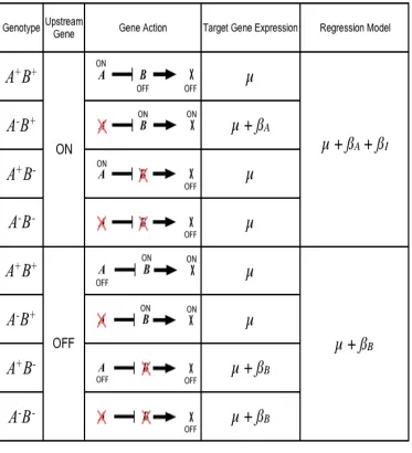
representing the presence or absence of each wild type allele and an interaction term. The interaction describes effects that are unique to the double mutant. The same example discussed above can be described as follows.

(39)

!

y=µ+"AxA +"BxB +"IxAxB +#

xA =

0for A+ 1 for A$

% &

' xB =

0for B+ 1for B$

% & '

Various techniques can be used to fit such a linear model. We first fit a full model

and then use stepwise backwards selection to drop model terms with coefficients that are not significant at a set level. The resulting reduced model is termed the best-fit model. For any

trait, there are eight possible best-fit models. For clarity, we number the reduced models as follows:

!

Model 1:y=µ+"A +# Model 2 :y=µ+"B +# Model 3 :y=µ+"I +# Model 4 :y=µ+"A +"B +# Model 5 :y=µ+"A +"I +# Model 6 :y=µ+"B +"I +# Model 7 :y=µ+"A +"B +"I +# Model 8 :y=µ+#

When the best-fit model has been determined, we estimate parameter values using

that model for each trait. Thus, we have a best-fit model and coefficient estimates for each trait. The terms in each best-fit model represent the significant gene and interaction effects acting on that trait. Individual coefficients represent the estimated effect of deleting each

gene. Model 7 corresponds to the classical model above when the interaction between the two deletions offsets the effect of one of them, either

!

"I =#"Aor

!

"I =#"B. Model 8

(40)

A best-fit model describes each gene expression trait. As such, we have dealt with the continuous variable problem. However, by embracing a quantitative genetic model we have lost the appealing feature of the classical experiment: the ability to interpret hierarchical

relationships. In the following section we identify sixteen hierarchical relationships and propose that a specific best-fit model supports each.

Interpreting Hierarchical Epistasis

In quantitative genetics, the interaction term in the above model is considered epistasis.

However, epistasis in this sense includes both hierarchical and nonhierarchical relationships. Conversely, while Model 7 can clearly be interpreted as hierarchical epistasis with the

conditions described above, it does not apply to all possible hierarchies.

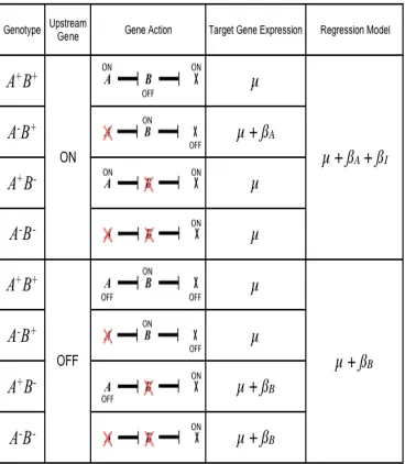
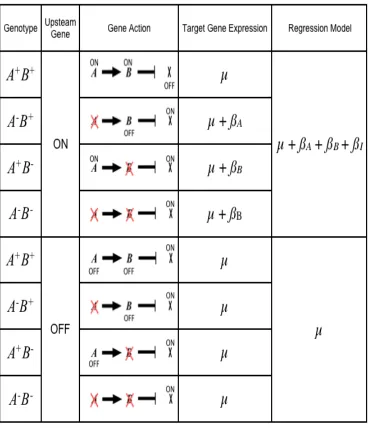
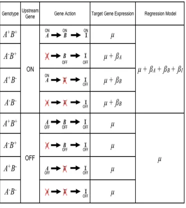
We considered all combinations of gene order and action within simple ON/OFF models and then predicted the hypothetical effect of deleting genes on each of them (Figures

2.1, 2.3, 2.4, 2.5). There are four points of variation to model for each gene pair relationship. The first is the identity of the upstream gene, i.e. the gene order. Secondly, the upstream

gene will turn the downstream gene either on (enhance) or off (repress). Thirdly, the

downstream gene can enhance or repress the expression of a target gene for which expression is observed. Lastly, we consider that the upstream gene itself will be enhanced or repressed

by some initiating factor such as a developmental cue or environmental perturbation. Avery and Wasserman (Avery and Wasserman 1992) provide a general framework that has been

(41)

does not give any information about whether the upstream gene is enhanced or repressed in that state. In our models, we focus on the effect on the upstream gene. This model has sixteen possible variants describing hierarchical relationships between two genes and the

(42)

Figure 2.1 Modeling the relationship A is an upstream repressor of B.

(43)

The key to our approach is connecting each of the sixteen hierarchical models to one of the eight possible best-fit regression models. If the deletion changes the state of a target gene relative to the wild type in a mutant, then that deletion is predicted to have a significant

effect and it will be included in the regression model corresponding to that hierarchical model. Figure 1 gives an example of one possible model, in which A is enhanced by a signal;

A is an upstream repressor to B; and B enhances a target gene X. We conclude that the

corresponding best-fit regression model will include coefficients for A and an interaction term. Note that if the signal instead represses A, a different best-fit model represents the

same relationship between A and B.

We applied the same approach to each of the sixteen cases and note several trends.

First, the downstream gene’s effect upon the target gene X does not influence the

corresponding best-fit model. This allows us to reduce the model space to eight hierarchical relationships (Table 2.1a). This observation is convenient, because expression traits

represent all the genes downstream of the deletions. Regardless of the downstream gene’s direct effect, some traits will be enhanced while others are repressed. When the upstream

gene is a repressor, four distinct regression models represent four unique hierarchical

relationships. We can uniquely identify both the gene order and signal effect on the upstream gene. We cannot discern gene order if the upstream gene is an enhancer because the same

(44)

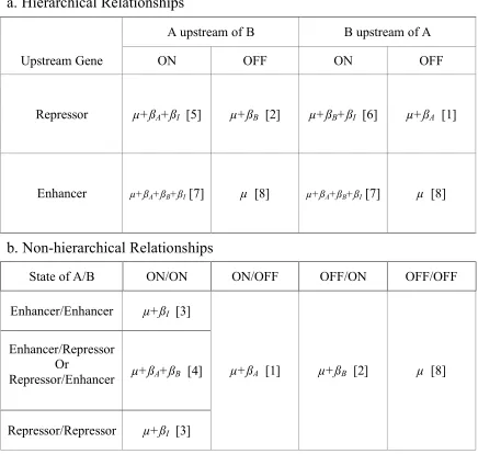
Table 2.1. Correspondence between regression models and biological models

a. Six of the eight possible regression models represent hierarchical relationships between genes. If the upstream gene is a repressor we can identify gene order and the signal effect. If the upstream gene is an enhancer, we can identify only the signal effect. If the signal turns off an upstream enhancer, deleting either gene will have no effect. b. Non-hierarchical relationships can be distinguished if both genes are activated by the signal. Model 3 suggests buffering, while Model 4 suggests independent effects, i.e. no epistasis. If a potential regulator is turned off by the signal it has no effect on the target gene.

a. Hierarchical Relationships

A upstream of B B upstream of A

Upstream Gene ON OFF ON OFF

Repressor µ+ßA+ßI [5] µ+ßB [2] µ+ßB+ßI [6] µ+ßA [1]

Enhancer µ+ßA+ßB+ßI [7] µ [8] µ+ßA+ßB+ßI [7] µ [8]

b. Non-hierarchical Relationships

State of A/B ON/ON ON/OFF OFF/ON OFF/OFF

Enhancer/Enhancer µ+ßI [3]

Enhancer/Repressor Or

Repressor/Enhancer µ+ßA+ßB [4]

Repressor/Repressor µ+ßI [3]

(45)

eight possible best-fit regression models correspond to the eight hierarchical relationships. It is notable that hierarchies can be indicated even without an interaction effect in the model.

We must also consider that there is no hierarchical relationship between A and B, or

that they do not affect the target gene (Table 2.1b). We can distinguish between two types of parallelism. Model 4, the two-gene additive model with no interaction, represents no

epistasis. Model 3 represents buffering epistasis, in which both genes act on the target in the same direction, and the effect of deleting either is not apparent unless both genes are deleted. We refer to this as nonhierarchical epistasis since neither gene is upstream of the other.

Deleting a deactivated regulator gene has no effect on the target gene, making it impossible to identify a biological relationship when regulators are deactivated.

The remainder of Table 2.1b represents cases in which one or both genes do not affect the target gene. Expression traits supporting Model 8 (no significant terms) may represent target genes that do not lie downstream of A or B, and are uninformative. The result is

one-to-many relationships between best-fit regression Models 1, 2, and 8 and their corresponding gene expression models. If the upstream gene of a hierarchical pair is turned off, we cannot

know whether it is upstream or uninvolved.

Typically, expression is measured from thousands of genes simultaneously and we do not expect them all to be informative. Even with clear interpretations for each trait

individually, there is a challenge interpreting all traits together. We examine the distribution of all traits. Among informative traits associated with a best-fit model, the majority may

(46)

Validating the Two-Step Modeling Framework

Van Driessche et al. used Dictyostellium discoideum wild type (Van Driessche et al. 2002) and deletion mutant strains (Van Driessche et al. 2005) to infer hierarchical epistasis

among genes of the protein kinase (PKA) pathway. Each strain’s gene expression profile was measured using cDNA microarrays with a common reference over 24 hours. These data

are well suited for testing our methods for two reasons. First, the epistatic relationships between the deleted genes already have been characterized experimentally. Secondly, the mutant strains are genetically identical at all loci except the few being studied, i.e. there is no

variation in their genetic background.

The PKA pathway is associated with the developmental aggregation response to

nutrient deprivation, which initiated midway through the time course. Data before and after aggregation were considered separately so we can clearly interpret the deletion effects in each signal state. The data represented fold-change on a logarithmic scale, which made the

distribution of expression measurements approximately normal; we consider the implications of this in the discussion. We studied 1553 expression traits. The genes we used were

measured in both experiments and differentially expressed in the wild type during aggregation (Van Driessche et al. 2002). Five deletion strains target genes of the protein kinase A (PKA) pathway that is involved in the response to starvation and activates

aggregation. This provided three contrasts: pufA/pkaC, pufA/yakA, and regA/pkaR. Although there are ten possible contrasts for these five genes, only these three double

(47)

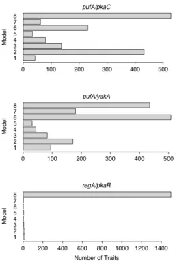
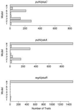
For each contrast, some traits supported each model (Figure 2). Additionally, large number of traits showed no deletion effects (i.e. support Model 8). At a significance threshold of p < 0.01, a majority of traits supported Model 8 for every contrast pre-aggregation (Figure S4)

and for the regA/pkaR contrast post-aggregation. According to our interpretive models, Model 8 can indicate three possibilities. The first two are hierarchical relationships in which

an upstream enhancing gene is turned off during aggregation. The last possibility is that the genes are uninvolved in the expression of the target and the deletions have no effect.

Since not all target genes are downstream of the PKA pathway, it is logical that the

deletions have no effect on these genes. Similarly, the PKA pathway is invoked during aggregation and it follows that the deletions may affect expression only after aggregation has

begun. We assume that the target genes supporting Model 8 are not downstream of the pathway, and that the majority of the remaining target genes reflect the relationship within the pathway. To test this assumption, we looked at the overlap between the expression traits

supporting Model 8 for each contrast. We found that all of the expression traits supporting Model 8 for the pufA/yakA contrast also supported Model 8 for the other two contrasts.

These traits strongly support the assumption that they are not downstream of the PKA pathway.

When we looked at these genes for both the pufA/pkaC and pufA/yakA contrasts, there

was strong support for one model over all others post-aggregation. Not only did these models explain more traits post-aggregation, but the models also fit better. On average, the

(48)

(49)

Figure 2.2 Post-aggregation distributions of best-fit models at p <0.01 significance thresholds

(50)

For the pufA/pkaC contrast, Model 2 had the most support of the seven non-null models. Model 2 corresponds to two possible interpretations. The first is that pkaC is the downstream

gene, that pufA is a repressor, and that the pufA is turned off in the presence of the

aggregation signal. Alternately, we could interpret it to mean that only pkaC has an effect on

the downstream targets and that pufA is unrelated. For the pufA/yakA contrast, Model 6 had the most support among non-null models. This model has a one-to-one correspondence to our interpretive models. It asserts that yakA is an upstream repressor of pufA, and that yakA

is turned on at aggregation. These conclusions both agree with what has been determined previously about the roles these three genes play during development (Souza et al. 1999).

YakA represses pufA, which then ceases to repress pkaC.

The regA/pkaR was problematic because almost all traits supported Model 8, the model with no effect terms. For the previous two cases, we assumed that these traits were

not downstream of the pathway. Given this assumption, we could have concluded that regA and pkaR were not involved with aggregation. However, the other two contrasts had 435 and

528 traits supporting Model 8, while regA/pkaR has 1497. Because of this discrepancy, we suggest that some proportion of these genes support the hierarchical model corresponding to Model 8: that one gene is an enhancer of the other and is deactivated by aggregation.

According to previously published results, regA and pkaR work together to repress pkaC pre-aggregation and are in fact deactivated post-pre-aggregation (Shaulsky et al. 1998). This is

consistent with the potential hierarchical relationship.

Because we are modeling nonadditive interactions, the logarithmic scale

(51)

(Frankel and Schork 1996; Lynch and Walsh 1998). To test this, we exponentiated the data and repeated our method. Despite dramatic changes to the shape of the data distribution, the resulting distribution of best-fit models agreed with the results presented above. Again, a

majority of traits showed no deletion effects (i.e. support Model 8). Model 2 had the most support for the pufA/pkaC contrast, Model 6 had the most support for the pufA/yakA contrast,

and Model 8 had near complete support for the regA/pkaR contrast using the

post-aggregation data (Figure S5). Interestingly, this does not imply that each trait supports the same model regardless of the scale transformation. In fact, only 57% and 47% of traits

support the same model with the untransformed data for the pufA/pkaC contrast and

pufA/yakA contrast respectively. However, in both these cases the vast majority of changed

traits support Model 8. This result amends our previous interpretation of the traits supporting Model 8; in addition to genes not downstream of the pathway, there may be some proportion of genes for which expression changes due to deletion is not detectable due to issues of scale.

Fewer traits supported Model 8 using transformed data, suggesting that these data may be more informative using the logarithmic transformation.

Thus, in all three cases our best-fit regression models correspond to a set of interpretative models that includes the true relationship between the genes. Certain

regression models have a one-to-many relationship with the interpretive models, but in these

cases the number of candidate interpretive models is reduced to a few. Only one

interpretation corresponds to Model 6, which makes the pufA/yakA contrast straightforward

(52)

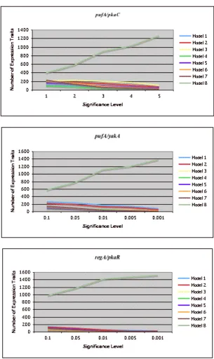
has an effect, the hierarchical model is a preferable interpretation to the pkaC only model. As we vary the significance threshold for model selection, our results are robust. The best-fit model among models 1-7 was the same for p-value thresholds from 0.05 to 0.001 (Figure

S6). As the selection criterion becomes stricter we reject more effects as not significant, and more traits support Model 8.

Discussion

Measuring transcript abundance within a cell will remain a fundamental interest to

biologists. Gene expression technologies have become popular over the past decade because of their ability to capture many genes simultaneously. Analyses that traditionally focused on a few genes now must be expanded to consider entire genomes. At this scale, the

relationships between genes are of as much interest as the genes’ individual effects. Many methods exist to infer gene networks or pathways from expression profiles (Bansal et al.

2007). Most of these require large datasets and result in large network diagrams that are difficult to interpret. These approaches are useful because they provide a genome scale view of transcription, and they are convenient because they can be applied to data from a variety

of easily accessible sources.

However, there is a continuing need for experiments that allow us to infer pathways

directly. The classical epistasis experiment we recount in our results (Van Driessche et al. 2005) is one such approach. Because it targets gene pairs directly, we can build pathways a relationship at a time. This local approach results in pathway diagrams that are easily