Abstract
Aman, Ronald L. A Minimal Surface Perturbation Method for Global Surface Registration of Unstructured Point Cloud Data. (Under the direction of Dr. Yuan-Shin
Lee.)
A MINIMAL SURFACE PERTURBATION METHOD FOR GLOBAL SURFACE REGISTRATION OF UNSTRUCTURED POINT CLOUD DATA.
By
Ronald L Aman
A thesis submitted to the Graduate Faculty of North Carolina State University
in partial fulfillment of the requirements for the Degree of Master of Science
INDUSTRIAL ENGINEERING
Raleigh 2004
Approved By:
_____________________________ _____________________________ Dr. Ezat T. Sanii Dr. Paul I. Ro
Dedication:
Biography:
Acknowledgments:
TABLE OF CONTENTS:
Page
List of Tables ...vii
List of Figures ...viii
Chapter 1 INTRODUCTION ...1
1.1 Introduction ...1
1.2 Organization of Thesis ...7
Chapter 2 LITERATURE REVIEW...8
2.1 Reverse Engineering ...8
2.2 Surface Registration...10
2.2.1 ICP Methods ...10
2.2.2 Newton Methods...12
2.2.4 Surface Signature Methods ...12
2.3 Surface Fitting...13
2.4 Surface Segmentation and Feature Recognition ...14
2.6 Neural Networks Techniques...14
2.7 Summary...16
Chapter 3 REGISTERING DATA FOR REVERSE ENGINEERING...17
3.1 Problem Statement ...17
3.2 Contact and Non-Contact Point Cloud Data Collection ...18
3.3 Data Preprocessing...24
3.4 Data Registration ...25
3.4.1 Generating the Geometric Handler ...26
3.4.2 Determining the Registration...26
3.5 Summary...29
Chapter 4 MINIMAL SURFACE PERTURBATION METHOD OF REGISTERING UNSTRUCTURED POINT CLOUD DATA...30
4.1 Introduction to Geometric Handler...30
Page
4.2.1 Initiation of Weights ...32
4.2.2 Geometric Weight Updating...34
4.3 Parameter Estimation ...36
4.4 Algorithm...37
4.5 Summary...43
Chapter 5 COMPUTER IMPLEMENTATION AND EXAMPLES...45
5.1 Implementation ...45
5.2 Examples...50
5.3 Summary...62
Chapter 6 CONCLUSION AND FUTURE WORK...63
6.1 Conclusions...63
6.2 Future Work ...64
List of Tables:
List of Figures:
Figure 1-1 Typical computer model generation...2
Figure 1-2 Object requiring multiple scans ...4
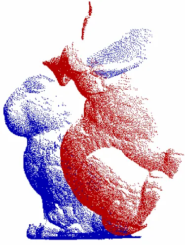
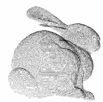
Figure 1-3 Data set representing Stanford bunny in two coord. frames ...5
Figure 2-1 Example 2 hidden layer neural network...15
Figure 3-1 Regular point cloud of data collected using laser scanning ...19
Figure 3-2 Data acquisition classes...20
Figure 3-3 Coordinate measuring machine example ...20
Figure 3-4 Laser scanner example ...21
Figure 3-5 Dense point cloud of Stanford bunny...22
Figure 3-6 Simulated difference between dense and sparse data ...23
Figure 3-7 Rotation and translation example...28
Figure 4-1 Point cloud and a geometric handler...31
Figure 4-2 Self-organizing map during training ...33
Figure 4-3 Dense data set with geometric handler...34
Figure 4-4 Update function neighborhood factor ...35
Figure 4-5 Example of estimating surface normal at the vertex...37
Figure 4-6 Creating the Geometric Handler flowchart ...39
Figure 5-1 Registration of furniture part...46
Figure 5-2 Generation of incorrect geometric handler ...48
Figure 5-3 Error caused by outlier eliminated ...49
Figure 5-4 Self-intersection occurring early in map generation ...50
Figure 5-5 Implementation of geometric handler on Stanford bunny ...51
Figure 5-6 Geometric handler without overlay of point data ...52
Figure 5-7 Geometric handler created with higher learning rate...53
Figure 5-8 Implementation of geometric handler for furniture part ...54
Figure 5-9 Furniture part prior to registration...55
Figure 5-10a Geometric handler with 20x20 grid...55
Figure 5-10b Geometric handler with surface normal approximations ...56
Figure 5-11 Registration of Die-cast mold ...57
Figure 5-12 Picture of die-cast mold ...57
Figure 5-13 Registration of vent hose...59
Figure 5-14 Picture of vent hose scanned for registration ...59
Figure 5-15 Side view vent hose after registration ...60
Figure 5-16 Vent hose example with error ...60
Figure 5-17 Die-cast mold example with 20x20 grid ...61
Chapter 1. INTRODUCTION
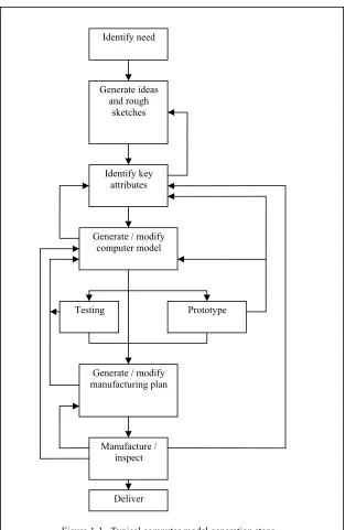
Computer Aided Design (CAD) models are an integral part of design and manufacturing today. They are used for development, testing and generating tools for manufacturing. Typically these models have been developed by a user drawing in a CAD program and take long periods of time for complex models. Reverse Engineering (RE) is a process which can generate CAD models by copying an existing part in a relatively short period of time, however one significant problem encountered in this process is that of data alignment of multiple dense point cloud sets. In this chapter, a brief introduction to the surface registration and data alignment problems is presented.
1.1 Introduction
Identify need
Generate ideas and rough
sketches
Identify key attributes
Generate / modify computer model
Generate / modify manufacturing plan
Manufacture / inspect
Prototype Testing
Deliver
Figure 1-1. Typical computer model generation steps.
computer systems. Models created in this way closely represent the part used as a pattern, or the ‘as built’ state.
Reverse engineering has many uses in design and manufacturing. Computer models generated using RE represent the part in the as built conditions, taking into consideration operations related to the manufacturing of the part (i.e. draft angles on sand cast parts, etc.). Reverse engineering parts today can take as little as a few hours, reducing costs significantly. In addition, parts that are defective from the standpoint of manufacturing inspection can be evaluated in analysis software (Finite Element Analysis, etc.) for final disposition. Potential scrap units may be evaluated as acceptable saving time and resources.
Capturing part data can be accomplished in general by using either contact or non-contact methods. Contact methods involve physical contact between the collection device and the part. These methods include manually measuring the part by an operator or Coordinate Measuring Machines (CMMs). Contact methods tend to be accurate, but provide data that is irregular (not collected in a predictable path or interval). Also some damage to the surface may occur because of the necessity of physical contact with the probe or measuring object.
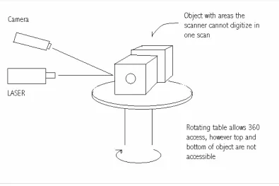
Figure 1-2. Example where multiple scans are required to collect data
for similar features or areas of similarity. This matching of overlapping sections is referred to in general as pose estimation or registration.
Registration of two overlapping data sets has several problems. First, registration techniques employ a minimization strategy to minimize the distance between the two data sets. Minimization techniques have a general tendency to become trapped in suboptimal solutions. This problem is magnified when random error is introduced, as is the case with many data collection techniques. Globally optimal solutions to the registration problem are required to minimize user interaction in these applications.
A second problem is identifying point correspondences across the two data sets. Point correspondence, used in the minimization of the distance between the data sets, is difficult because it is highly unlikely that two data points in different sets represents the exact same location of the model. In other words, even though the underlying surfaces corresponding to two separate scans of an object are identical, the point clouds may not coincide due to the difference in relative orientation of the scanning patterns. This problem arises because of the discrete nature of data collection.
The surface registration problem is applicable to many disciplines. Computer vision (stereo vision), computer graphics, image processing, and reverse engineering and quality inspection are examples of areas currently implementing surface registration techniques. Improved registration techniques will lead to more autonomous systems and more accuracy within these systems.
minimizing the distance between the data sets; however this can lead to localized point matching, not the ideal matching of the overlapping sections of the data sets. The minimal surface perturbation method generates a geometric handler that approximates the data set reducing surface deviations and reducing the impact of random error. These geometric handlers are then registered thus finding an approximate registration of the global shape of the sets.
1.2 Organization of Thesis
Chapter 2. LITERATURE REVIEW
In this chapter, the previous work related to surface registration in relation to reverse engineering is presented. The related techniques of surface registration, including surface fitting, surface segmentation, feature recognition, and surface matching along with methods of surface registration are introduced.
2.1. Reverse Engineering
Reverse Engineering (RE) is the process of decomposing an existing part or system to gain greater understanding of the characteristics or operations of the part or system. In this study, it involves making a copy of an existing object in the form of a computer model for further analysis, design or manufacturing use. Creating the computer model involves several major steps including capturing the data, segmenting the data into regions, fitting surfaces to the segmented regions, and creating the CAD representation for use in various operations. For a complete introduction into reverse engineering, see the review work done by [Varady 97].
Huang and Menq (2003) present a system by which a CAD model is reconstructed from multiple point clouds [Huang 03]. The system includes shape recovery, mesh segmentation and CAD model construction. The shape recovery is performed by estimating parameters in a local area by utilizing a nearest neighbor algorithm to search for points located in the neighborhood. These points are then used to estimate parameters such as surface normal and local curvature. These parameters are used for the segmentation and shape recovery.
Yau et al (2000) discuss the reconstruction of point data for complex 3D models where the overlapping points in each point cloud must be eliminated to maintain density requirements [Yau 00]. This is especially important in the case where a tessellated model is a step between integration of the points and creating a surface. Li et al (2002) present a rapid manufacturing process where a point cloud is used to generate a tessellated surface for rapid prototyping [Li 02].
To define a computer model, Benko et al (2002) present numerical methods of constrained fitting in reverse engineering where primitives as well as sweeps are used [Benko 02]. A set of normalization and shape constraints are used in conjunction with external geometric constraints for fitting surfaces. The implementation uses a list of constraints to be applied to primary surfaces that have been identified by some technique, and point data that has been previously segmented for the various surfaces.
regularities that may be present based on the primary and secondary objects is determined individually and the list is examined to find inconsistent constraints. The inconsistent regularities are then rejected.
Thompson et al (1999) present a method for generating a computer model based on features from a point cloud of data for reverse engineering [Thompson 99]. User specifies regions where features exist to build the model. The features are defined by use of individual primitives and some combinations of primitives (e.g. two different sized coaxial cylinders represent a counter bore). This system is limited to several types of 2 ½-D features.
2.2 Surface Registration
In the past decade, research in the field of surface registration has primarily been conducted for computer vision or metrology [Tucker 03a]. Surface registration techniques may be broken down into several categories. Methods related to the Iterative Closest Point (ICP) method are the most popular. Other methods include Newton methods, neural network methods and surface signature methods. In the following sections the related methods used for surface registration are discussed.
2.2.1. ICP Methods
Other algorithms such as Singular Value Decomposition (SVD) are acceptable substitutes for the quaternion-based algorithm [Besl 92]. This method is applied iteratively until the sum of square distances between the data sets is minimized (square distance function is used to eliminate problematic negative values). The determination of the related points in each data set (those which are the closest) is problematic. In this case, they use those points that are closest by Euclidean distance. This can create some problems if the data sets are poorly aligned early in the process, leading to a locally optimal registration.
This method has been expanded with many different variations. Some reduce the computation time of finding the point sets by choosing a small subset of each total point set to compare. Several methods have been proposed including uniform sampling of points [Turk 94], random sampling of points [Masuda 96], and high deviation of the estimated surface normal [Rusinkiewicz 01]. Chen and Medioni (1991) use an approximation to the source points normal to find the intersection of a ray with the opposite surface [Chen 91]. Blais and Levine (1995) used the view of the scanner to create a ray from the point to the scanner and intersect this ray with the opposing surface [Blais 95].
2.2.2 Newton Methods
Tucker and Kurfess (2003a, 2003b) present a pure Newton’s method approach to the registration problem [Tucker 03a, 03b]. This technique uses various Newton methods including full Newton, Quasi-Newton, and Gauss-Newton methods to minimize the squared distance between a cloud of points and a surface by solving a Taylor’s series expansion of the distance function using first and second order derivatives to find the registration. These methods are faster than the ICP method, but are applicable for point to parametric surface registration. Like the ICP methods, these methods must have an accurate initial approximation to converge to the correct registration.
Gunnarsson and Prinz (1987) present a technique implementing a Newton method [Gunnarsson 87]. They used a finite difference computation approximating derivative data that significantly increased computation time as the number of points grew [Tucker 03a].
2.2.3. Surface Signature Methods
Yamany and Farag (2002) present a method of using surface signatures to identify corresponding areas within data sets [Yamany 02]. A surface signature for each point is generated containing an angular and distance relationship to every other point on the surface. The surface signature uses the curvature at each point requiring an accurate estimate of this parameter. In the case of parametric surfaces, this is not a problem. In the case of noisy data, estimating surface curvature accurately is problematic.
(1996), Johnson and Herbert (1999) and Stein and Medioni (1992) all generate a signature map of the data which can be used for registration [Chua 96, Johnson 99, Stein 92]. The difficulty with these methods is finding a robust surface signature, especially in noisy data.
2.3 Surface Fitting
Many research results have been published regarding the fitting of surfaces, for an introduction to surface fitting see the books by [Zeid 91, Piegl 95]. More complex surfaces and more complex methods to fit surfaces have been published recently. Wang, Chang and Yuen (2000) present a fuzzy distance function to identify feature regions and fit surfaces to a human model [Wang 00]. The surface model is maintained as a polygon mesh. Patrikalakis and Maekawa (2002) provides theory and algorithms for constructing Bezier, B-Spline and NURBS curves and surfaces [Patrikalakis 02].
2.4 Surface Segmentation and Feature Recognition
Surface segmentation and feature recognition are very closely related. Segmentation is defined as partitioning the set of all points in a data set into n regions containing m points such that the union of all regions is the point set, and every point resides in exactly one region [Yokoya 89]. In general, segmentation techniques can be divided into five categories; Thresholding, Edge-Based, Region-Based, Range Data Segmentation, and Neural Network [Zhongwei 03].
Besl and Jain (1987) developed a method by which an image was viewed as a piecewise smooth surface [Besl 87]. Zhongwei and Shouwei (2003) present a method which fits a Non-Uniform Rational B-Spline (NURBS) surface using an ordered point data set as control points [Zhongwei 03]. The surface normal and curvature are evaluated on the surface represented by a 2D image. The regions can then be determined by finding areas of similarity within the image.
2.5 Neural Networks Techniques
ANNs are a computer implementation simulating the live connectivity between nervous cells. An input signal is directed to a node which depending on the input generates an output. The neighboring nodes also receive the input and generate an output. The combined signals are sent to another layer of nodes, which acts similarly. Any number of central layer nodes may exist. A final set of nodes known as the output nodes creates the necessary output signal based on the input and the combined actions of the central nodes. Figure 2-1 shows an example 2 hidden layer feed forward neural network. There are a large number of different ANN implementations; several popular versions are the backpropagation of errors, radial basis function, and self-organizing maps [Aliev 01].
Figure 2-1. Example 2 hidden layer neural network.
Neural networks have been used recently in finding approximate solutions to non-linear problems. Examples include segmentation of data, identification, image processing, pattern recognition, surface registration, robotics control systems and speech / word recognition [Kecman 01]. Wachowiak et al (2002) present the use of a Radial Basis Function neural network to estimate the registration of medical images, including the registration from a patient to an atlas [Wachowiak 02].
Input
Hidden layers (2)
Qian and Li (1992) present a method using a binary Hopfield neural network to register complex images [Qian 92]. The network used to identify interesting point matches within each image. The point matches are then used to find the rotation and translation transformation that leads to the lowest energy as defined by difference between the images in the overlapping area. Piraino et al (1994) applies a feed-forward back-propagation neural network to determine the rotation and translation matrices [Piraino 94]. This method was found to be accurate for linear space transformations, but the necessity of point-to-point correspondence reduced its feasibility. Also non-linear transformations were found to be not as accurate.
2.6 Summary
Chapter 3. REGISTERING DATA FOR REVERSE
ENGINEERING
In this chapter, a new method for surface registration is presented. A definition of the surface registration problem, background regarding collection of point cloud data, data processing as related to the registration problem, and a new method of registration utilizing a geometric handler are presented in the following sections.
3.1 Problem Statement
In the global surface registration problem, two problems are intertwined. The first problem is to identify those portions of the data sets that overlap in a meaningful way, and the second one is to find the transformation that creates a best fit merging of the overlapped portions. This thesis primarily focuses on the second.
Consider two sets of coordinate points P and Q containing n and m points respectively,
P = {p1, p2, p3, …, pn; pi∈ℜ3} (1)
and
Q = {q1, q2, q3, …, qm; qj∈ℜ3}. (2)
θy, θz and a translation vector T as a function of tx, ty, tz such that the distance F satisfies
the following conditions:
F(R, T) = Σ(pi– Rqi+T)2 pi ⊂ P and qi ⊂ Q (3)
R = f(θx, θy, θz)3x3 (4)
T = (tx, ty, tz)T (5)
Minimizing F(R,T) refers to overlapping portions of data sets P and Q, where θ represents an angle of rotation about the respective axis, and t represents a transposition along the respective axis.
Minimization techniques employed may lead to local optimal solution when conditions are unfavorable [Tucker 03a, Besl 92]. Unfavorable conditions include poor initial starting locations of the data sets, significant noise in the data and existing outliers. A global shape recognition and registration will reduce the effects of the noise as well as local surface shape changes, thus reducing the importance of the starting point for the correct registration.
3.2 Contact and Non-Contact Point Cloud Data Collection
Data representing an object is normally collected in what is called a point cloud. Point clouds generally consist of a number of Cartesian space vectors originating at the origin and ending at the intersection of the part. In 3D data collection, it is normally described in terms of an x coordinate, y coordinate, and a z coordinate. Thus
represents a point in space where a line originating from the origin intersects an object. The set of points described by equation (1) provides a discrete representation of an objects surface in 3 dimensions (Figure 3-1).
Figure 3-1. Regular point cloud collected using laser scanning
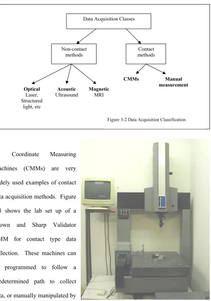
Coordinate Measuring Machines (CMMs) are very widely used examples of contact data acquisition methods. Figure 3-3 shows the lab set up of a Brown and Sharp Validator CMM for contact type data collection. These machines can be programmed to follow a predetermined path to collect data, or manually manipulated by an operator to collect data points
Data Acquisition Classes
Non-contact
methods methods Contact
CMMs Manual
measurement Optical Laser, Structured light, etc Acoustic
Ultrasound Magnetic MRI
Figure 3-2 Data Acquisition Classification
[Groover 02]. The data collected using CMMs is often used for inspection purposes in metrology. Because these machines are built as rigid structures and because of the physical contact between the measuring instrument and the part, random data error is kept minimal (as compared to non-contact methods).
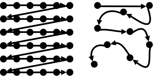
Data is considered regular or structured if the interval between points is predictable in some way. Non-contact data is normally collected such that a small distance separates each collected point in a sequential pattern (Figure 3-5). The result is a dense structured point cloud representing an object (Figures 3-5 and 3-6). The scanner in our lab is capable of collecting point data at 0.008inch intervals and has an accuracy of approximately 0.009inch.
Figure 3-5. Dense point cloud of the Stanford bunny captured using
Figure 3-6. Simulated collection routes of 3D point data.
Regardless of the care in collecting data, some errors will occur. The random errors in the data are often referred to as white noise or noise. These errors occur for many reasons such as vibration in measuring equipment and changes in the atmosphere. This noise is problematic when attempting to generate a smooth, continuous and accurate representation from discrete point data.
3.3 Data Preprocessing
In this section, the techniques of data processing practices are discussed. Processing of data may be necessary to correct for some inherent problems in the data such as noise, occlusions and outlying points.
Once data is collected in point clouds, it may need some processing to remove noise and outliers or to restore areas of missing data. Many filtering approaches exist to reduce high frequency noise. Reducing noise should be avoided during early stages of reverse engineering to minimize the elimination of good data points, especially in sharp corners. Noise in the data is not removed in the minimal surface perturbation method of registering point data because of the difficulty in discerning noise from accurate data. Elimination of accurate data, especially in areas such as corner points where there is a significant change in the surface direction, is unwanted.
Identifying outlying points is important in the data processing step. Outlying points can be quantified differently, but in general they are considered a single or small group of points lying a significant distance from the majority of the points. These points may be errors caused by the data collection method, such as when a through hole is digitized using a laser scanner, or may represent real data from a distant surface. To minimize the impact of the registration caused by outlying points, our geometric handler will not consider points located a given distance from the mean surface.
in Rapid Prototyping (RP) as input to build RP models. The tessellated surface is also useful for segmenting data because of built in relationships between triangle surfaces, and the ease of which one can estimate parameters such as surface normal and curvature.
3.4 Data Registration
Many current registration techniques are based on minimizing the distance between some set of points in each cloud. Minimization techniques have a tendency to become trapped in local minima while searching for the global minimum. This may require registration attempts using many different starting positions to find the correct transformation, or require outside user input to identify a good starting position. Correct transformation and resulting registration is necessary to eliminate user input for completely automated tasks such as quality inspection.
Local registration techniques have been developed and enhanced such that computation is relatively fast [Besl 92, Tucker 03]. Global registration has not been as fully studied. The tendency of current algorithms to find sub-optimal solutions leads to user interaction as preferable substitute to searching for the global registration.
3.4.1. Generating the Geometric Handlers
To process unorganized point clouds, the “geometric handlers” is proposed for quick and efficient handling of huge amounts of data [Aman 04a]. The geometric handlers are a surface approximation aimed at finding global shape of the point cloud data. The geometric handler is a smaller set of points with some connectivity between the points that can be used to reduce the size of the data set to be registered while maintaining the overall topology (global shape) of the point cloud. The characteristics of interest for this geometric handler are; maintenance of the global shape, organization of the points, connectivity amongst the points, and capable of use for registration. As will be explained in further detail in Chapter 4, the Kohonen self-organizing neural network provide these attributes [Aman 04b].
Assuming we now have two sets of ordered points we set out to determine R and T to minimize the distance between each data set. In the following sections, methods for registration of organized point data will be presented.
3.4.2 Determining the Registration
The SVD method requires the calculation of a cross-covariance matrix for subsequent decomposition into eigenvectors. The maximum eigenvector corresponds to the rotation which minimizes the deviation of the points in the two data sets. The cross covariance matrix is determined after finding the centroid of each data set:
∑
= = n i i c p n P 1 1 (7)∑
= = n i i c q n Q 1 1 (8)The cross-covariance matrix, H, is then:
(
) (
)
∑
= − −= ni i c T
c
i P q Q
p
H 1 (9)
The cross covariance matrix, H, can then be decomposed into three matrices using a process called singular value decomposition:
T V U
H = Λ (10)
where U and V are orthonormal 3x3 matrices representing the eigenvectors, and Λ is a 3x3 non-negative diagonal matrix of singular values. Each orthonormal matrix along with the corresponding singular value represents the principle axis of a hyper-sphere deformed into a hyper-ellipse. Multiplying the two orthonormal matrices then results in a rotation corresponding to the rotation of the axis of the hyper-sphere to the principle axis of the hyper-ellipse. The rotation matrix R can then be determined:
T VU
R= (11)
c
c RP
Q
T = − (12)
Where Qc and Pc are defined by equations (7) and (8). This system can be iteratively
applied to get a closer approximation to the registration, however since this is a global approximation to the registration, the local registration will used to optimize the registration. More details of searching for the global optimal surface registration will be discussed in Chapter 4.
The cleanliness of this method is based on the point clouds having an ordered correspondence to one another. In general, point clouds rarely have such correspondence. This makes the use of the geometric handler a very important part of using this method. The geometric handler should create an ordered point cloud capable of having correspondence across multiple data sets. The Kohonen self-organizing map described in Chapter 4 performs this function.
Figure 3-7. Description of rotation and translation T
Qc
R*Pc (Dashed)
3.5 Summary
Chapter 4. MINIMAL SURFACE PERTURBATION
METHOD FOR REGISTERING UNSTRUCTURED POINT
CLOUD DATA
In this chapter, the minimal surface perturbation method for registering unstructured point cloud data is discussed. The previous section discussed the method by which an ordered point cloud containing the same number of points, with point correspondence is registered. This chapter will focus on the generation of the geometric handler and the metrics by which it is developed.
4.1 Introduction to Geometric Handler
Figure 4-1. Point cloud of 15,400 points and geometric handler using a 10x10 grid.
The geometric handler registration will lead to a global registration of the point clouds. The relatively large distance between points in the geometric handler leads to errors in the registration. Performing a local registration using the neighborhood found by the geometric handler improves the registration.
4.2 Geometric Handler Creation
4.2.1 Initialization of the Weights
The weights of the neural network are represented as the intersection of any two lines in figure 4-2 (a-f). The weights for each geometric handler are initialized to a starting value. For the purpose of this research, random weight values were assigned for generality (Figure 4-2a). In practice, a more suitable approach to initialization may be choosing random points within the data set for faster convergence.
Weight i j∈ℜ3 (13)
Initialization of the weights is done once for each geometric handler at the beginning of the algorithm.
a) Point cloud to be approximated (Rotated down 30°)
b) Initial state – random values for weights
c) after 25 iterations – weights organizing but self-intesecting.
d) after 100 iterations – self intersection worked out
e) after 250 iterations
f) after 1000 iterations – final state
4.2.2 Geometric Weight Updating
To approximate a point cloud data set, a randomly chosen point from the data set is input to the neural network. The neural network finds the closest weight and ‘updates’ this weight and a neighborhood of surrounding weights to more closely represent the input point. The process is repeated a set number of iterations.
The neural network is applied in two stages. In the first stage the neighborhood is larger and the ‘update’ is more significant. In the second stage the neighborhood
includes only the weight on each side of the closest weight, and the amount ‘updated’ is reduced. In each stage the update amount is reduced as the cycle progresses.
Updating occurs in the following way: The distance d between the randomly chosen point and the closest weight is calculated (this can be either positive or negative). The neighborhood weights γ are moved by an amount determined by the update function:
γ= γ + K*( d )*Γ (14)
Γ = e-(number of points away from center of neighborhood)
K = linearly decreasing damping value (learning rate)
The starting neighborhood is defined as the smaller of the width of the weight array or the length of the weight array. The neighborhood is reduced in equal amounts regularly until only the immediate points surrounding the chosen weight are updated. In the case where the neighborhood is 5 points, the update values range from 1 at the center point to .243 at the edges.
5 3
1 -1 -3
-55 3 1 -1 -3 -5 0 0.2 0.4 0.6 0.8 1
Update as a percentage of
distance
nuber of points aw ay from center
num ber of points aw ay from center
Figure 4-4. Update Function Neighborhood Factor
The learning rate K plays an important role in generating the geometric handler. If the learning rate is too low, the map may be unable to overcome a self-intersecting situation. If the learning rate is too high the geometric handler may become self-intersecting. In general this value is assigned a starting value in the neighborhood of 1.0, and decreases linearly to a smaller value near 0.1 for the first phase. For phase two the learning rate starts near the value where phase 1 ended and decreases towards 0.
Each phase (phase 1 and 2) are performed a specified number of times. Phase 1 has a larger impact on the global shape of the geometric handler. Phase 2 enhances the local approximation.
4.3 Parameter Estimation
Parameters of the geometric handler can be estimated using segments between weights. Each weight represents a corner of a polyhedron. The normal vector at each corner of the polyhedron is found by use of cross product. The 4 normal vectors for a specific polyhedron are averaged and the result is unitized. This is used as the estimate of the normal vector for the polyhedron.
The parameter estimations can be used to identify areas of similarity. The organized structure of the geometric handler makes it easy to navigate from potential matching pairs in one data set to neighboring pairs.
Figure 4-5 example of estimating surface normals at the vertex.
4.4 Algorithm
In this section the algorithms implemented for testing the proposed method are described. Figure 4-5 shows the flow chart for the algorithm for creating the geometric handler. For the geometric handler creation, a random point from the point cloud is chosen, the closest weight is found and the weight neighborhood is updated. The amount the weights are moved during each iteration is then reduced, and at specified intervals the number of points in the neighborhood is reduced. At this point another random point is chosen and the process continues until the specified number of iterations is reached.
Once the geometric handler is generated, the registration method of SVD is invoked. If the registration error (the difference between the geometric handlers) is large,
e1
e2
e4
e3
N1 = e2 X e1
N2 = e3 X e2
N3 = e4 X e3
N4 = e1 X e4
Choose Random Point
Find Closest Weight
Update the Weight Neighborhood
Determine Distance between Weight
and Point
Done?
Output
Reduce Update Factor Reduce
Neighborhood Size if Necessary
Point set Create Geometric Handler
Figure 4-6. Creating the Geometric Handler Yes
Algorithm I. Geometric Handler Construction Algorithm
Input
• Number of weights to represent data.
• Data in x y z format
• Number of iterations for Phase 1 (P1)
• Number of iterations for Phase 2 (P2)
Output – 2-dimensional array of weights representing original data
Step 1. Chose a point at random from point set. Step 2. Find the weight closest to the chosen point. Step 3. Update the weight (for x, y and z)
K= stepping variable (17)
λ = learning rate (18)
Φ(x) = K * λ*(point– weight) (16) weight = weight + Φ(x) (15)
Step 4. Update the weights surrounding the closest weight using Φ.
β is an exponentially decaying factor as distance from the closest weight increases
Step 5. Perform steps 1-4 a preset number of times (125) Step 6. Update K linearly from 0.9 to 0.1 by δK.
K = K - δK (20)
δK = (0.9-0.1) / (P1) (21)
Step 7. Perform the steps 1 through 5 P1 times (phase 1 iterations)
Step 8. Repeat the above steps updating only one weight on each side of chosen weight in step 5, and updating K linearly from .1 to 0.
δK = (0.1-0.0) / (P2) (22)
Step 9. Repeat steps one through seven for the second data set. END.
Algorithm II. SVD Registration of the Geometric Handlers.
Input –
Two data sets, P and Q, with an equal number of weights (n) generated by the Geometric Handler Construction Algorithm above.
Output –
Rotation and translation matrices
Step 1. Find the centroid of each data set P and Q, pc and qc.
pc = (1/n) Σipi (23) qc = (1/n) Σiqi (24)
Step 2. Calculate the cross covariance matrix H
H= Σi (pi - pc)T(qi - qc), i = 1…n (25)
Step 3. Find the singular value decomposition of H
H = UΛVT (26)
Step 4. Calculate rotation matrix R
Step 5. Find the translation vector
T0 = qc – R0pc. (28)
Step 6. Repeat steps above to minimize the sum of squares error. END.
Algorithm II is used to find the rotation matrix and translation vector for the transformation of the geometric handler for data set P. The centroids of the weight set are the average of the values of all the weights. Then as shown in Arun et al (1987), two sets of data, one a rotation and translation of the other, will have the same centroid. Determining the rotation involves finding three matrices, two orthonormal and one diagonal matrix with all positive values that when multiplied together yields the matrix
H. The two-orthonormal matrices can then be multiplied to come up with the rotation matrix. The rotation matrix can then be applied to the centroid of one data set and subtracting the two will yield the translation vector.
4.5 Summary
Chapter 5. COMPUTER IMPLEMENTATION AND
EXAMPLES
In this chapter, the computer implementation will be presented. Details regarding the results and displays of geometric handler are presented. Example parts showing good results and those which were evaluated during testing are presented.
5.1 Implementation
Implementation of the proposed method was done in Microsoft Visual C++ 6.0 run on a Pentium 3 866Mhz PC. A partial scan of a furniture part was made using a laser scanner. The interesting portion of the scan was cropped and the resulting data set copied and rotated for testing. The resulting scan contained 15,400 points and was approximated using a 10x10 grid of weights. The data set and resulting geometric handlers are displayed in Figure 5-1. The transformation was determined and applied resulting in a sum square error (SSE) of 49.708. The mean square error (MSE) was 0.00331, resulting in an error of approximately 3%.
∑
= −= ni qi
SSE 1 2
i ) p
( (29)
(
)
1 2 1 − − =∑
= n q p MSE ni i i (30)
Table 5-1 Results of testing
No. of points No. of weights CPU Time SSE MSE SVD SSE 441 100 (10x10) 45 seconds 4.40 0.00998 2.71 15400 256 (16x16) 5 min 20
sec
50.407 0.00331 49.1587 15400 144 (12x12) 2 min 27
sec
Comparisons were made with the straight SVD method where the points were known to correspond within the two data sets. The SSE of 49.1587 for the SVD method reflects error added to simulate noise in the data (normally distributed centered about zero with standard deviation of 0.05).
Testing of the map generation revealed several important factors. First, outliers play a significant roll in the generation of the geometric handler. As Figure 5-2 shows, a point located below and to the left looking at the image pulls the geometric handler away from a global approximation to the point data. This results in a poor geometric handler being created. Restricting the maximum amount a point can move in one iteration eliminates the incorrect mapping (Figure 5-3).
Figure 5-4. Self-intersection occurs early in the map creation process. As is shown in figure 4-2, the geometric handler corrects the self-intersection and correctly represents the point cloud data.
5.2 Examples
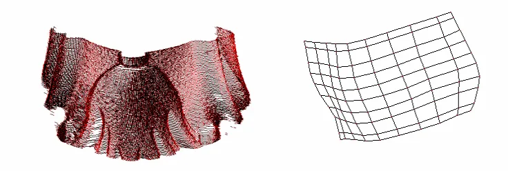
Figure 5-5 Exmple geometric handler on the Stanford bunny utilizing a 20x20 grid. Map is less
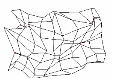
Figure 5-7 Example part with surface normal approximations.
The geometric handler does a good job of approximating the point clouds. As seen in Figure 5-8, the details of the furniture part create very little change in the surface estimated by the geometric handler. This smoothness creates fewer details for the registration to become trapped. The result of the reduced surface perturbations is that of fewer wild surface normal changes in small regions caused by random data error. This allows better global surface approximation.
Figure 5-9 shows two geometric handlers of similar parts. Figure 5-10(a) shows the geometric handler (20x20) approximating the furniture part. Figure 5-10(b) shows
Areas of low density with very few weights approximating in this area
Surface normal
approximations. The normal approximations accurately display the smooth change of the overall shape of the point cloud without rapid changes caused by noise.
Figure 5-9 Two furniture parts with geometric handlers prior to registration
Figure 5-10b a 20x20 geometric handler with a good approximation and surface normal approximations.
Further examples for registration were generated by scanning a die-casting mold (Figure 5-12) using the Roland Picza scanner in our lab. The scan was performed in a planar fashion, collecting data from only one side of the mold resulting in 20800 points collected. The scan was then copied and rotated to simulate a scan from a different orientation. A 15x15 mesh geometric handler was used for the registration (Figure 5-11). The resulting error between the two data sets was .0011202inch(overall dimension of mold 4.5inch x 4.5inch). Further examples of the die-cast mold using a 20x20 grid and a 12x12 are also shown (Figures 5-17 and 5-18).
Figure 5-11 Die-casting mold scanned using laser scanner in Industrial Engineering Metrology Lab.
Figure 5-12 Die-cast mold used for scanning.
many surface perturbations (Figure 5-14). The global shape of the hose is captured using a 15x15 mesh grid representing 9119 points (figures 5-13 and 5-15). The registration error between all corresponding points is 0.0007656inch (overall dimensions 4inch x 5 inch). The registration was run several times on the same data with similar results. In some cases the error was larger, to 138.858inch total (Figure 5-16). This resulted in an average error of .015inch per point in the data set, well within the local minima area of the proper registration solution. Ten registration trials yielded an average total error of 154.14inch (sum of the square root of the square Euclidean distance between
corresponding point pairs) and an average point error of .0169inch (total error / number of points) using a 15x15 grid.
Grid size
15x15 10x10 6x6 4x4 3x3
Average point error
Of 10 registration iterations 0.016903 0.010884 4.46E-09 6.3E-09 7.7E-09
Figure 5-15 Side view of vent hose data points after registration.
Figure 5-17 Die-cast mold cavity registered using 20x20 grid
5.3 Summary
Chapter 6. CONCLUSION
6.1 Conclusion
In this paper, the “geometric handler” and the “minimal surface perturbation method” have been proposed for the global registration approximation of unorganized point cloud data sets. Initial results of the minimal surface perturbation method are promising. Given two unstructured overlapping data sets, a geometric handler is generated to approximate each data set. The geometric handler has an organized structure such that neighboring points are easy to identify. Using this structure, a transformation can be found to minimize the distance between the geometric handlers. This transformation can be used as a starting point for other registration methods.
6.2 Future work
The point cloud approximation allows us to easily find the estimated surface normals and a representation of the curvature of the global object. This and similar surface properties will be required to register two point clouds that have only a partial overlap. To extend the proposed method for handling such data sets, the geometric handler may provide a convenient starting point. Typically, local matching of surface properties based on tessellated models requires some form of sub-graph matching. By first using the sparser geometric handler, this step can be speeded up significantly to obtain an initial, crude registration. In the future research, the exploration and implementation of this method is forthcoming.
References
[Aliev 01] Aliev RA, Aliev RR “Soft Computing and its Applications.” Singapore: World Scientific 2001.
[Aman 04a] Aman RL, Joneja A, Lee YS. “Unorganized Point Registration Using Kohonen Neural Network” Computers in Industry - In Review
[Aman 04b] Aman RL, Joneja A, Lee YS. “Minimal Surface Perturbation Registration of Unorganized Points” ASME IMECE Conference November 2004 - In Review
[Arun 87] Arun, K.S., Huang, T.S., and Blostein, S.D., “Least-squares fitting two 3-D point sets,” IEEE Transaction on Pattern Analysis and Machine Intelligence, vol. 9, pp. 698-700
[Au 99] C.K. Au and M.M.F. Yuen , “Feature-based reserve engineering of mannequin for garment design.” Computer Aided Design Vol. 31 no.12 (1999), pp. 751–759
[Barhak 01] Barhak J, Fischer A “Parameterization and Reconstruction form 3D scattered Points Based on Neural Network and PDE techniques” IEEE Transactions on Visualization and Computer Graphics Vol. 7, no. 1 (2001)
[Benko 01] Benko P, Martin RR, Varady T. “Algorithms for Reverse Engineering Boundary Representation Models.” Computer Aided Design Vol. 33, (2001), pp. 839-851.
[Benko 02] Benko P, Kos G, Varady T, Ando, L, Martin R. “Constrained fitting in Reverse Engineering.” Computer Aided Geometric Design, Vol. 19 (2002), pp. 173-205.
[Besl 87] Besl, P and Jain, R “Segmentation and classification of range images”
IEEE Transactions on Pattern Analysis and machine Intelligence Vol. 9 (1987) pp. 608-620
[Besl 92] Besl, P. and McKay, N. “A Method for Registration of 3-D Shapes,”
Trans. PAMI, Vol.14, No.2, Feb. 1992
[Carr 01] J. C. Carr, R. K. Beatson, J.B. Cherrie, T. J. Mitchell, W. R. Fright, B. C. McCallum and T. R. Evans “Reconstruction and Representation of 3D objects with Radial Basis Functions.” ACM SIGGRAPH 2001, pp.67-76,
[Chau 96] Chua CS “3D Free-Form Surface Registration and Object Recognition.” Int. Journal of Computer Vision Vol. 17, 1996, pp. 77-99
[Chen 91] Chen, Y. and Medioni, G. “Object Modeling by Registration of Multiple range images,” Proc. IEEE Conf. On Robotics and Automation, 1991
[Fisher 04] Fisher RB. “Applying Knowledge to Reverse Engineering Problems.”
Computer Aided Design, Vol. 36, no. 6, 2004, pp. 501-510.
[Ghosh 02] Ghosh A, Pal S. “Soft Computing Approach to Pattern Recognition and Image Processing.” World Scientific Publishing Co. Pte. Ltd. Singapore, 2002
[Groover 01] Groover, M. “Fundementals of Modern Manufacturing. Second Edtion” NY: John Wiley and Sons, 2002.
[Gunnarsson 87] Gunnarsson KT, Friedrich BP. CAD model based localization of parts in manufacturing. Computer 1987; 20(8):66-74.
[Heskes 01] Heskes, Tom. “Self-Organizing Maps, Vector Quantization, and Mixture Modeling.” IEEE Transactions on Neural Networks Vol. 12, no. 6 (2001) pp. 1299-1305
[Huang 03] Huang J, Menq JH, “Automatic CAD Model Reconstruction from Multiple Point Clouds for Reverse Engineering.” 2003 NSF Design, Service, and Manufacturing Grantees and Research Conference Proceedings, pp. 318-333.
[Kecman 01] Kecman, V. “Learning and Soft Computing. Support Vector Machines, Neural Networks, and Fuzzy Logic Models.” The MIT Press, Cambridge, Mass. 2001
[Knopf 01] Knopf G, Al-Naji R. “Adaptive Reconstruction of Bone Geometry from Serial Cross Sections.” Artificial Intelligence in Engineering
Vol.15 (2001) pp. 227-239
[Kohonen 96] Kohonen T, Oja E, Simula O, Visa A, Kangas J. “Engineering Applications of the Self-Organizing Map.” Proceedings of the IEEE
Vol. 84, no. 10
[Langbein 04] Langbein FC, Marshall AD, Martin RR. “Choosing Consistent Constraints for Beautification of Reverse Engineered Geometric Models.” Computer Aided Design Vol. 36 (2004), pp. 261-278.
[Li 02] Li L, Schemenauer N, Peng X, Zeng Y, Gu P. “A Reverse Engineering System for Rapid Manufacturing of Complex Objects.” Robotics and Computer Integrated Manufacturing, Vol. 18, (2002), pp. 53-67. [Masuda 96] Masuda, T. Sakaue, K., and Yokoya, N. “Registration and Integration
of Multiple Range Images for 3-D Model Construction,” Proc. CVPR, 1996
[Pal 99] Pal S, Mitra S. “Neuro-Fuzzy Pattern Recognition; Methods in Soft Computing.” John Wiley and Sons, NY 1999
[Patrikalakis 02] Patrikalakis NM, Maekawa T, “Shape Interrogation for Computer Aided Design and Manufacturing.” Springer, New York, 2002.
[Piegl 95] Piegl LA and Tiller W. “The NURBS Book.” Spriger, New York 1995 [Piraino 94] Piraino, D., Kotsas, P., Richmond, B., Recht, M, Kormos, D., “Three
Dimensional Image Registration Using Artificial Neural Networks,”
IEEE 1994
[Rusinkiewicz 01] Rusinkiewicz, Szymon and Levoy, Marc “Efficient variants of the ICP Algorithm,” 3Dim Conference on Image Processing, 2001
[Su 00] Su MC, Chang HT. “Fast Self-Organizing Feature Map Algorithm.”
IEEE Transactions on Neural Networks Vol. 11, no. 3 (2000) pp. 721 – 733
[Suganthan 02] Suganthan, PN. “Shape Indexing using Self-organizing Maps.” IEEE Transactions on Neural Networks Vol. 13, no. 4 (2002) pp. 835-840 [Thompson 99] Thompson WB, Owens JC, de St. Germain HJ, Stark SR, Henderson
TC. “Feature-Based Reverse Engineering of Mechanical Parts.” IEEE Transactions on Robotics and Automation, Vol. 15, no. 1, 1999, pp. 57-66.
[Tucker 03a] Tucker, Thomas M and Kurfess, Thomas R. “Newton Methods for Parametric Surface registration. Part I.” Computer Aided Design, Vol. 35, no. 1, 2003, pp. 107-114
[Turk, 94] Turk, G. and Levoy, Marc M. “Zippered Polygon Meshes from Range Images,” Proc. SIGGRAPH, 1994
[Varady 97] Varady T, Martin R, and Cox J. “Reverse Engineering of Geometric Models – an Introduction” Computer Aided Design, Vol. 29, no. 4, 1997, pp. 255-268.
[Wachowiak 02] Wachowiak, Mark P., Smoliková, Renata, Zurada, Jacek M., Elmaghraby, Adel s. “A Supervised Learning Approach to Landmark-Based Elastic Biomedical Image Registration and Interpolation,”
Neural Networks, 2002. IJCNN '02. Proceedings of the 2002 International Joint Conference on, 2002 pp. 1625 -1630 vol.2
[Wang 03] Wang CL, Chang TK and Yuen MF “From laser-scanned data to feature human model: a system based on fuzzy logic concept”,
Computer-Aided Design, Volume 35, no. 3 (2003) pp. 241-253
[Yamany 02] Yamany SM and Farag A, “Surface Signatures: An Orientation Independent Free-Form Surface Representation Scheme for the Purpose of Objects Registration and Matching.” IEEE Transactions on Pattern Analysis and Machine Intelligence Vol. 24, no. 8, (2002) pp. 1105-1120
[Yau 00] Yau HT, Chen CY, Wilhelm RG. “Registration and Integration of Multiple Laser Scanned Data for Reverse Engineering of Complex 3D Models.” Int. Journal of Production Research Vol.30 no.2 (2000) pp. 269-285
[Yokoya 89] Yokoya, N and Levine, D. “Range Image Segmentation based on differential geometry: A Hybrid Approach. IEEE Transactions on Pattern Analysis and machine intelligence Vol. 11 (1989) pp. 643-649 [Zeid 91] Zeid “CAD/CAM Theory and Practice” McGraw Hill. NY, NY 1991 [Zhongwei 03 ] Zhongwei Y, Shouwei J. “Automatic Segmentation and approximation
of Digitized Data for Reverse Engineering.” Int. Journal Prod. Research Vol.14, no. 13 pp. 3045-3058.