Modeling multiple conductor transmission lines

Modeling Multiple Conductor Transmission Lines

Michael LeRoy Riddle

Center for Communications and Signal Processing

Department of Computer Science

North Carolina State University

ccsr-

TR-88/16

TABLE OF CONlENTS

Abstract

III

List of Figures

1

v

List of Abbreviations and Symbols

v

Chapter 1 -- Introduction

1

Chapter

2 --

Review of Single Conductor Theory

3

Chapter

3 --

Multiple Conductor Systems

1

0

Section 1 -- Impedance-Voltage Method.

1

0

Section

2 -- Paul's State Variable Method

1 7

Section

3 --

Gruner's Method

20

Summary --

24

Chapter

4 -- Numerical Simulation and Comparison

with

Actual

Measurements

.

26

Test

1 A --

2

7

Test

1 B

-~

.

2 7

Test

1

C -- .

2 8

Test

1 D -- .

2

8

Comments on Theoretical vs.

Measured

Results

3 3

Test

1 A --

3 3

Test

1 B -- .

3

5

Test 1

C -- .

3 6

Test 1 D -- .

3 6

Paul's

and Gruner's Methods

3 7

Comments .

3

7

Chapter

5 --

Conclusions

4

1

Notes

62

Bibliography

64

Abstract

This

paper will present a new

way

of modeling multiple

conductor transmission lines.

Actual physical measurements will be

used to verify the theory.

Chapter 1 will summarize the current

state of research.

Chapter

2

will review the behavior of single

conductor systems.

Chapter 3 will present three approaches to

LIST OF FIGURES

Figure 1 -- A single conductor transmission system .

3

Figure 2 -- Distributed line parameters

4

Figure 3 -- Equivalent circuit for single conductor line at x

=

O.

7

Figure 4 -- Per unit parameters for a two conductor system

.

1 1

Figure 5 -- Boundary conditions at source for multiple conductors 1 3

Figure 6 -- Load for a two conductor system

.

1 6

Figure 7 -- Gruner's circuit model for two conductors

.

2 1

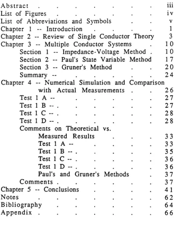
Figure 8 -- Configuration for Test 1A

. 2 7

Figure 9 -- Configuration for Test IB

. 2 7

Figure 10 -- Configuration for Test 1C

.

2 8

Figure 11 -- Configuration for Test ID

. 2 8

Plot 1(a) -- Theoretical voltage vs. distance (Test #lA)

. 4 3

Plot l(b) -- Theoretical current vs. distance (Test

#.lA)

.

44

Plot l(c) -- Measured voltage vs. distance (Test #lA)

. 45

Plot

led) --

Measured current vs. distance (Test

#lA)

.

4 6

Plot 2(a) -- Theoretical voltage vs. distance (Test #lB)

. 4 7

Plot 2(b) -- Theoretical current vs. distance (Test #lB)

. 4 8

Plot 2(c) -- Measured voltage vs. distance (Test #lB)

.

4 9

Plot 2(d) -- Measured current vs. distance (Test #lB)

.

5 0

Plot 3(a) -- Theoretical voltage vs. distance (Test #1 C)

. 5 1

Plot 3(b) -- Theoretical current vs. distance (Test #lC)

. 5 2

Plot 3(c) -- Measured voltage vs, distance (Test #lC)

.

5

3

LIST OF SYNIBOLS

Z -- per unit impedance matrix

Y -- per unit admittance matrix

r --

reflection coefficient matrix

Zo -- characteristic impedance matrix

y

0 --

characteristic admittance matrix

ZL --

load impedance matrix, also referred to as receivmg end

impedance

matrix

Y

L

--

load admittance matrix, also referred to as receiving end

admittance

matrix

Z

s --

source impedance matrix, also referred to as sending end

impedance

matrix

y

s --

source admittance matrix, also referred to as sending end

admittance

matrix

y -- propagation constant matrix

V +

forward travelling voltage wave vector

w

V

backward travelling voltage wave vector

w

I

+

forward travelling current wave vector

w

I

backward travelling current wave vector

w

d

F --

derivative of F, i.e. dx F(x)

G(x,~)

-- Green's function matrix

V

s --

source voltage vector

Is

source current vector

U -- unity matrix

C1>

--

transition matrix

Chapter

1

Introd uction

An electrical transmission line is an electromagnetic medium

which serves to guide the flow of energy from one point to another.

The equations governing this system are ultimately derived from

Maxwell's equations, but usually it is more convenient to derive

them

by

applying circuit theory.

Equations describing single

conductor systems have been developed and extensively researched

[1,2].

Although several final forms of the equations exist and related

notation is not standardized, one can show

~

with some algebraic

manipulation, that these seemingly different equations are

In

fact

equivalent.

Of equal importance, these mathematical models have

been verified through associated empirical work [3,4].

complications resulting from standing wave patterns.

At present,

methods for predicting what these patterns will be on

multiconductor utility networks are lacking or inadequate.

While there has been research in characterizing multiple

conductor lines [5-15], the theory thus far developed has not lent

itself well to computer simulations of complex networks.

The matrix

equations used to describe these systems require considerable

computer resources which has

not

been widely available until

recently.

Another problem has been the form of the equations

themselves.

While they adequately describe

the

behavior of

the

line

(as will be shown

in chapter

3),

their

form

is somewhat cumbersome.

Consequently,

they

do not allow for

ready extension

to network

systems.

Finally, research to compare the theory

with

measurements

of actual systems has

been

almost non-existent.

This paper will provide a set of equations

modeling

multiple

conductor systems which extends directly

from

single

conductor

circuit theory.

They are relatively compact and can easily be

used

to

Chapter

2

Review

of Single

Conductor

Theory

This chapter will review the theory governing single conductor

systems such as that shown in Figure 1.

The parameters that we

know are the source voltage and the two terminations.

In addition,

we have some description of the parameters of the transmission line

itself.

What we are trying to solve for is the voltage and current at

...

...---.I(L)

l

any point along the line.

I(O)~

o

L

v,

V(O)

V(L)

Figure 1 -- A single conductor transmission system.

complete description of the characteristics of the line, we can now

proceed to solve the system of equations describing it.

r

~x

1

z x

ao----~x

r

~x l~x

r

~x

1

z.x

Figure 2 -- Distributed line parameters.

Two differential equations can be written to describe the

behavior of this circuit.

V'(x)

=

-Z I(x)

I'(x)

= -

y Vex)

The general solution for these equations is [1,2]:

+

-

'VY

Vex)

=

V

e-yx.

+

Veil.

w

w

where

r

=

~

Zy

is the propagation constant.

(1)

(2)

(3)

(4)

v"

and 1+ are referred to as the forward travelling voltage and

w

w

current waves, and V

and 1-

are referred to as the backward

travelling voltage and current waves.

These are defined with respect

.ish some relationships between

tension of circuit theory we know

d current waves will be related

o.

This will also be true for the

ent waves, and thus we can

(5)

a

(5) b

Zo

=

Y-ly=

Zr

l

This allows us to rewrite equations (3) and (4) as:

lex)

=

L(v+

e-

YX -

v:

e

YX )

Zo

w

w

(5)

c

(6)

(7)

Another relationship which we can define between the

reflection coefficient is defined as the ratio between the forward and

backward travelling voltage waves.

Specifically, it is:

v

w

")

rex)

= -

e,,·:y(x-L)

(8)

v+

w

It follows then that equation (6) can be rewritten as:

+

Vex)

=

V

_w

e-Yx

[1

+

rex)]

₍₉₎

and at the beginning of the line, we can write an equation for V(O)

simply as:

(10)

and from

here we can easily write a transfer function for the system:

(11 )

and

likewise for the current:

( 12)

While the transfer function

IS

useful, especially in numerical

First, we can also write

YeO)

in terms of the sending end

termination

Zs

and the effective input impedance

Zin(O)

of the

system at its sending end.

But, first we must define the input

impedance at all points along the line.

This is done by simply finding

V(x)/I(x), and it can be shown that in general this will be:

1

+

rex)

Zin(X)

=

ZOI _

r

(X )

(13)

Notice that the equivalent circuit at x=O becomes as shown

In

Figure 3 below.

1(0)

~

o

t - + - - - . .

V

(0 )

Figure 3 -- Equivalent circuit for single conductor line at x=O.

This implies

that:

1

+

rco)

Zin(O)

=

ZOI _ reO)

and from Figure 3

it is easy to see that:

YeO)

= V

s

Zin(O)

Zs

+

Zin(O)

(14 )

Substituting, we obtain:

Vex)

=

V

s Zin(O)

e-Yx

(l

+

rex))

z,

+

Zin(O)

(1

+

reO))

We can now

define the reflection coefficient at each

termination

as:

r -

Zs - Zo

s -Zs

+

Zo

and

In addition, we can

see that rex) can be defined by:

r(x)

=

rL e2y(x-L)

And again substituting as appropriate, we can write:

In

the same way, we can find an expression for the current:

and a

more useful expression for the input impedance:

(16)

(17)

(18 )

(19 )

(20)

(21 )

1

+

rLe 21'(x-L )

Z:

(x) -

Zo

(22)

In -

1 _

rLe 2y(x-L)

of the

system,

including

the

net effect

of

any

and all reflections

on

the line.

By

also having them in a transfer function form and

by

having a closed form expression for the input impedance at the

beginning of the line, large networks can be constructed and

analyzed at any point on the network.

A program called CAPNET

[3,4] has been developed which does exactly this.

In the next

Chapter

3

Multiple

Conductor

Systems

This chapter will present three methods for determining the

voltage and current at any point along multiple conductor

transmission lines.

Section 1 will review the Impedance-Voltage

Method which simply extends the model of the previous chapter to

multiple

conductors.

Section

1 --

Impedance-Voltage

Method.

First, let us consider how we will characterize the line itself.

In

chapter 2 we worked with the Per Unit Impedance and Admittance.

This

proved

to

be

quite convenient, and

we

can extend the concept of

per

unit

values to multiple

conductor

systems.

Figure 4 shows

a

two

conductor system and illustrates how the parameters relate to one

another.

N

otice

that this implies that we must now express all

parameters in matrix farm.

Also notice that the coupling between

lines is expressed in two parts.

Y12

represents capacitive coupling

between line 1 and line 2, and

Z12

represents inductive coupling

between

them.

Applying some simple circuit theory and

USIng

linear algebra

preceding chapter.

First, we have two differential equations of the

form:

V'(x) ::: -Z

1(0)

I'(x)

=

-y YeO)

which are exactly the same as for the single conductor case.

However, for multiple conductors V and I are vectors of n length

where n is the number of conductors (not including the ground

plane), and Z and Yare n x

n matrices of the form:

(23)

y

11

dx

Zll

dx

r0'

Y12

_ZlZ

_dx

_!

dx

J

ZzzdX

'0'

Y 22

dx

J

!

I

IJ

aii

i

~

+

2

r

Again, paralleling the development for the single conductor

case, the general solution for this differential equation is:

Vex)

=

e-yx.

v:

+

e"(X

v:

w

w

. -yx

+

yx.

•

Itx)

=

Y

0

e

I

_{w -}

Yo

e

I

_w

(24)

a

(24) b

where

Vex)

and

lex)

are the voltage and current vectors,

respectively.

V+

and 1+ are the forward travelling voltage and

w

w

current waves.

V

and 1-

are the backward travelling voltage and

w

w

current waves.

We can now define the reflection coefficient and

input impedance at any point along the line.

rex)

e-"(X

v~

=

erx

V~

V~

=

e-yx.

rex)

e-rx

v~

and

Vex)

=

z.

(x)

lex)

In

These are:

(25)

a

(25) b

(26)

From this last equation we can derive the relationship:

which gives us an alternate way of defining

rex).

That is:

(27)

From the boundary conditions at the source (shown In Figure

5),

we can see that:

-1

V(O) = Zin(O) [

z,

+

Zin(O)]

V

_s

(29 )

and

that

Vex) = [

u

+

rex)]

e-

rx

V;

₍₃₀₎

V(O)= [ U

+

r(Q] V:

_{(31 )}

-1

V: = [

u

+

reO)]

V(O)

₍₃₂₎

1(0)

~

o

...---..V(O)

Figure 5 -- Boundary conditions

at

source

for

multiple conductors.

It then follows that

and hence that

-1

Z. (x) = [

u

+

rex) ][

u -

r(x)] Z

In

0

(33)

and at the load, i.e. at x

=

L we have

r ., r ,-1

Z.

(L)

=

ZL

= I U

+

rn.:

!

i

U -

rn.:

JI

Z

ill ~ ....

0

= [

U

+

r

L] [

U -

r

L

r

Zo

This allows us to further write:

r(x)

=

e-y(x-L)

r

e-y(x-L)

L

and so at x

=

0:

(35 )

(36)

(37)

(38)

a

(38) b

Substituting as appropriate, we finally arnve at a complete

solution.

and

[ U

y(x-L)

r

Y(X-L)]

-yx [

U _

e-yL

r

e -yL

r

lZ

I(x)

=

Yo

-

e

L e e

L

J

0

[ z,

+ (

U

+

e-yL

r

L e -yL ) (

U -

e-yL

r

L e-yL

J

1

Zo

J

1

(41 )

However, once again for purposes of simulating large networks,

these equations

are

more useful in their transfer

function

form:

-1

Vex)

= [

U

+

e"f{x-L)

r

L ey(x-L) ] e-Yx [

U

+

e-yL

r

L e-YL]

YeO)

- 1

lex)

=

Y

0 [

U -

e ')'(x-L)

r

L e ')'(x-L) ] e -yx [

U -

e -yL

r

L e

-)i.] ;

1(0)

Some consideration needs to be

given

to the terminations.

( 42)

As

stated earlier, these will be modeled as n

x

n matrices.

The question

then anses as to how we determine their exact form.

First, let us consider the load termination, such as the two

conductor load shown in Figure 6.

Notice that the load has been

defined in terms of admittances.

This is strictly for convenience.

(It

could also have been defined

In terms of impedances, but finding an

expression is more difficult.)

Applying Kirchhoffs voltage and

current laws, we obtain:

I(L)

= YL

V(L)

where

(43)

.f'

it

I

(L)

YL11

YL12

(L)

YL22

I

x=L

Figure 6 -- Load for a two conductor system.

In general, we can show that for n

conductors,

Y

_{1I + Y12 + ·· · +}

Y

l n

-Y

_{1 2}

-YIn

- y

1 2

Y

22

+

Y

1:;

+ ... +

Y

2n

-

y

2 n

-y

₁

-y

Y

+

Y

+ ...

Y

n (n-1 )n nn 1n (n-l)n

For impedances,

VeL)

=

ZL

I(L)

where

(46 )

(47)

The situation

IS

considerably more complex with the source

termination.

This is because of the greater number of permutations

of possible configurations, i.e. one could have

a

voltage source in

series with impedances or

a

current source in parallel with

admittances or something

else.

However,

by

drawing out the

configuration and applying Kirchhoffs laws, Z, or Y

s

can be properly

determined.

There are several advantages to having the equations In the

impedance-voltage form.

For one, arbitrary load conditions can

be

handled.

In addition, it is easy to apply

them

to a n=l single

conductor system and show that

they

reduce to the exact same

equations as shown in the previous chapter.

Also, they are relatively

easy to implement in a computer simulation, and can be readily

extended to complex networks.

Section 2 -- Paul's State Variable Method [14].

matrix.

In this approach, we set up the differential equations

governing the system as:

-Z]

[V(X)]

On

lex)

(48 )

and from state

variable theory,

we know that the general form of

the

solution to this equation

IS:

where

<1>11' <1>12' <1>21'

and

<1>22

are n x n matrices.

Paul goes on to show that

the

elements

of

<1>

are:

-1

<t>

(x)

=

-Y

cosh(yx) Y

11

<1>12(x)

=

-Zo

sinh(yx)

.. 1

<1> 21 (x)

=-

sinh(yx)

Zo

<1> 2/x)

=

cosh(yx)

where again

y

=

..Jyz

( 49)

(50)

(50)

a

(50) b

(50)

c

In section 1,

y was said to equal

...j

YZ and this same definition

has been used in this section.

One might ask

if it could not just as

easily be defined as

...j

ZY.

The answer is yes.

Paul explains that a

parallel development exists for the case where

y

=

...j

ZY. Using linear

algebra theory, one can show that the same general equations as

presented in this and the preceding section hold.

The only change

IS

that

Zo

must also be redefined to

Zo

=

'Y

y-l

=

r 1

z.

Having defined all the elements of

<t>

one has only to solve for

YeO)

and 1(0) in order to compute

Vex) and I(x).

Equations (29) and

(38) from the preceding section can be used to do this.

With a little algebraic manipulation, it can be shown that Paul's

equations can be reduced in the single conductor case to exactly

those presented in chapter 2.

Presumably they will reduce as well

for the multiple conductor case, but the degree of complexity in

demonstrating this increases dramatically.

However, in numerical

simulation of the same data sets, both Paul's method and the

impedance-voltage method produce nearly identical results.

The principle advantage of the impedance-voltage method

IS In

Matrix Operation

Volt.-Imped.

State-Trans.

exponent

2

2

add/subtract

2

2

muttipty

2

2

transpose

0

1

vector add/subtract

0

2

vector

multiply

4

4

scalar

multiply

0

2

Total operations

10

₁₅

Chart 1 -- Comparison of number of matrix operations.

Section 3 --

Gruner's method

[15].

Paul's method begins

by

dealing strictly with the transmission

line itself.

Consideration of meeting boundary conditions is handled

after first developing necessary equations to describe the behavior of

the line itself.

The effects of the terminations ultimately are taken

into account in solving for V(O) and 1(0).

The impedance-voltage

method takes the effects of terminations into account along the way

Gruner begins by defining the differential equation describing

the change in voltage and current as one moves away from the

source in his circuit model shown in Figure 7.

This is given by:

r

~(x)]

=

[On

L

I(x)

-v

-z] [

V(X)]

+

[V

~

On

I(x)

IsJ

(51 )

where

V

s

and

Is

are the distributed input voltage and current

sources.

,---,

I I

I I I

I

I I

1'1

Ys12

I

4,:

I t

I I I I I I

it

I I

IV

1

(L)

YL11

I

I

i

~

.

(L)

: -7 11

L12

r

:V

2(L)

L22

I I

i~

I I

I ,

t---1

x=O

x=L

From two-point boundary value theory, we know that the

general solution of a system of the form y'

=

Ay

+

f(x), subject to

two

point boundary conditions Way(a)

+

Wby(b)

=

0, has a solution of the

form:

b

y(x)

=

J

G(x,~)f(~) d~

a

where

-1

a

-1

G(x,~)

=

cI>(x) D W <I>(a)<1>

(~),

G(X,~)

=-cI>(X)

D-IWbcI>(b)cI>-l(~),

(52)

(53)

a

(53) b

<I>

(x), WS, WL, D, and

G(x,~)

are 2n x 2n matrices.

<1>(x) represents an

arbitrary fundamental

matrix from the homogeneous counterpart of

(51).

Gruner determines

<I>(x) to

be:

<1>(x)

=

cosh(yx)

-sinhC'''?x) [yT] "v

-sinh(yx)

y-l

Z

cosh(yTx)

(54 )

which

is equivalent to equation

(50)

given by Paul.

However, Gruner

goes on to say that there are computational advantages to using a

different fundamental matrix

which

he gives as:

(55 )

Gruner does not show exactly how he obtained this equation,

but in two computer simulations, one

using

equation (54) and the

other using equation (55).. nearly the same answers were obtained.

Additionally, using equation (55)

and

assuming only one conductor,

one can obtain the exact set of equations as shown in chapter 2.

(This is

done

by

assuming

Is

=

0 and

Es(~)

=

Vs , i.e. applied voltage is

only at the source end which implies that

~

=

0.) [15]

W

S

is derived from the source boundary conditions and

In

the

case of Figure 7 is:

s

[U

W=

On

(56)

W

L

is derived from the load boundary conditions and

In

the

case of Figure 7 is:

(57)

D is defined by:

D =

WS<I>(O)

+

WL<1>(L)

and for Figure 7 is equal to:

(58)

D=

U +ZsY

_o

-yL

_yT

_L

e

-';'e

Yo

u -

ZsY

_o

yL

yT

_L

e

+

ZL

e

Yo

Substituting as appropriate, we now have

G(x,~):

G

12(X,~)

G22(X,~)

(60)

For the single conductor case with only a voltage source at the

source end, one can show that Gruner's approach leads

to

exactly the

same equations as obtained in section 1 of this chapter.

Once again,

the equations in section

1-

have a computational advantage and some

advantage

in intuitive presentation.

However, Gruner's method can

easily be extended to

a variety of line situations.

In

particular,

it can

handle both distributed voltage and current sources at any point

along the line.

However, without equations for input impedance such

as those derived in section

l , it is difficult, at best, to extend this

approach to

complex multiconductor networks.

Summary

complex network systems.

However, as the next chapter will

show,

Chapter

4

Numerical

Simulation

and

Comparison

with

Actual

Measurements

The equations presented

In

the previous chapter have been

developed into four computer simulations:

( 1) A simulation based on the equations In section 1.

(Appendix

A)

(2) A

simulation based on Paul's approach.

(Appendix

B)

(3)

Two simulations based on Gruner's approach.

(a) One using Gruner's full fundamental matrix

~

as

given

in equation

(54).

(Appendix

C)

(b)

One using Gruner's simplified fundamental matrix

<I>

as

given in equation (55).

(Appendix D)

Test 1

A

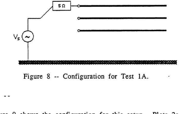
--Figure 8 shows the configuration for this setup.

Plots 1a and

1b show the theoretical voltage and current along

the line.

Plots 1c

and ld show the actual measured voltage and current on the line.

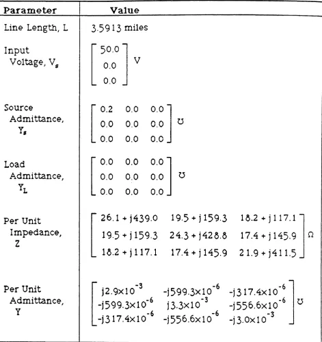
Table 1 gives the parameters used for the simulation.

o

Figure 8 -- Configuration for Test

lA.

Test 1 B

Test 1

C

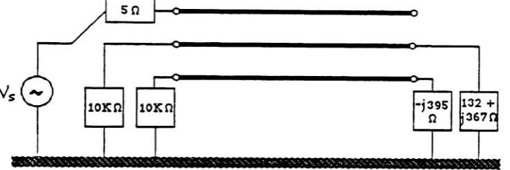
--Figure 10 shows the configuration for this setup.

Plots 3a and

3b show the theoretical voltage and current along the line.

Plots 3c

and 3d show the actual measured voltage and current on the line.

Table

3

gives the parameters used

for

the simulation.

Figure 10 -- Configuration for

Test

1C.

Test 1 D

--Figure

11 shows the

configuration for

this setup.

Plots

4a

and

4b show

the

theoretical

voltage and

current along

the line.

Plots

4c

and 4d show the

actual

measured voltage and current on the

line.

Table 4 gives the parameters used

for the

simulation.

Parameter

Value

Line

Length,

L

3.5913

miles

-

-Input

50.0

Voltage}

v.

_0.0

V

~

0.0 _

Source

- 0.2

0.0

0.0

-Admittance,

0.0

0.0

0.0

U

y.

0.0 _

_ 0.0

0.0

-

-Load

0.0

0.0

0.0

Admittance}

0.0

0.0

0.0

U

Y

_L

_{... 0.0}

0.0

0.0 _

Per

Unit

- 26.1

+

j439.0

19·5

+

j

159·3

la.2+j117.1-Impedance,

_19.5

₊

_j

_159.3

_{24.3 + j42a.&}

_{17.4 +}

_{j 145.9}

_n

Z

_ la.2+j117.1

17.4

+

j

145.9

21.9+j411.5_

--

-3

-6

-6

Per Unit

_j2.9x

₁₀

_-j599.3xIO

_-j

_317.4xl

₀

Admittance,

-6

-3

-6

_U

-jS99.3xlO

j3.3xIO

-j556.6xIO

y

_-6

_-6

_-3

-j317.4xI0

-j556.6xIO

-j

3.0x

10

-

Parameter

_Value

Line Length, L

_{3·59 13}

_miles

~

-Input

50.0

Voltage} V

_s

_50.0

V

50.0

-

-Source

,

-0.2

0.0

0.0

-Admittance,

0.0

0.2

0.0

U

Y

s

-. 0.0

0.0

0.2 _

-

_0.0

_0.0

_0.0

-Load

Admittance,

0.0

0.0

0.0

U

Y

_l

_{-. 0.0}

_0.0

_{0.0 _}

Per Unit

- 26.1

+

j439.0

19·5 ...

j

159.3

1a.2

+

j

11 7.1

-Impedance}

_19.5

₊

_j

_159.3

_24.3

₊

_j428.8

_17.4+j145.9

n

Z

17.4 +

j

145.9

21.9+j411.5 _

__ 18.2

+

j

117.1

--

-3

-6

-6

Per Unit

j

2

.9xl 0

-j599.3xIO

-i317.4xIO

Admittance,

-6

-3

-6

_1<.5

-j599.3xIO

j

3.3x

10

-j556.6xIO

y

_-6

-6

-3

-j317.4xI0

-j556.6xI0

-j3.0xlO

-

Parameter

Value

3.59

13

miles

-Line Length, L

Input

Voltage} V

_s

Source

Admittance}

y.

Load

Admittance.

Y

_L

-

-50.0

0.0

_ 0.0 _

-

_0.2

0.0

_ 0.0

-

_0.0

0.0

.. 0.0

v

0.0

-6

IOO.OxIO

0.0

0.0

-3

-j2.0xIO

0.0

0.0

0.0

t5

-6

IOO.OxlO

_

0.0

0.0

U

.

-3

-]2.0 xl 0

_

Per Unit

Impedance,

Z

- 26.1

+

j439.0

19.5

+

j

159.3

... 16.2+j117.1

1

9.5

+

j

159.3

24.3

+

j42~.a

17.4

+

j

145.9

18.2

+

j

117.1

-17.4+j145.9

o

21.9+j411.5_

-Per Unit

Admittance,

y

-

-3

j2.9x

10

-6

-jS99.3xl0

-6

-j317.4xIO

--6

-6

-j599.3xIO

-j317.4xIO

-3

-6

0

j3.3xIO

-j556.6xIO

-6

-3

-j556.6xIO

-j3.0xIO

Parameter

Line Lengtn. L

Input

Voltage

l

V.

Source

Admittance.

Y

s

Load

Admittance.

Y

_L

Value

3.5913

miles

-

-50.0

50.0

V

50.0

-.

-

,.-0.2

0.0

0.0

-0.0

0.2

0.0

U

... 0.0

0.0

0.2 _

~

0.0

0.0

0.0

-0.0

-j

2.0

x

10

-3

0.0

U

_ 0.0

_0.0

-]2.0xIO

.

-3

_

Per Unit

Impedance,

Z

- 26.1

+

j439.0

19.5

+

j

159.3

__ 1a.2

+

j 11 7. 1

1

9.5

+

j

159.3

24.3

+

j4Za.8

17.4+j145.9

1~.2+j117.1­

17.4+j145.9

n

21.9+j411.5_

Per Unit

Admittance

l

y

--

-3

-6

-6

j2.9xIO

-j599.3

x 1O

-j317-4x

10

-6

-3

-6

U

-j599.3

x 1O

j3.3xlO

-j556.6xIO

-6

-6

-3

-j317.4xIO

-j556.6xI0

-j3·

0x 1O

Comments

on

Theoretical

vs.

Measured

Results

.-Overall there was some disparity between the theoretical

predictions and the actual measurements.

Before discussing possible

reasons for this and their implications, let us first briefly compare

them.

Test

lA:

Voltage Curves -- The measurements show marked variation

on phase A, which was the only phase to have voltage

applied to it

in

this test., while phases Band C remained

relatively constant at around 16V.

The pattern observed on

phase

A

is generally what we would expect for

a

line

terminated in an

open

circuit.

Physically it

IS

approximately

one

half wavelength.

This

indicates that the propagation

velocity along the line is very close to the speed of light,

since the physical wavelength is nearly equal to the

theoretical one, i.e.

(3.0

x

10

8

_{m/sec)/(25kHz)}

_(25kHz

_was

the frequency of the sinusoidal voltage generator in the

experiment.).

Also there is no perceptible damping,

i.e.

the

line appears to be relatively lossless.

The pattern observed

on phases Band

C

is more difficult to explain.

It was

higher than on phase A.

This has not yet been fully

explained.

The theoretical predictions parallel the measurements

only

loosely.

Phase

A

shows

the

general standing wave pattern

for an open circuit, but also seems to show that the line

IS

slightly longer than one half wavelength.

While the

beginning point is also at 50V, it is at a different point

along

the line.

Thus, the voltage rises somewhat before falling,

unlike the measurements which clearly show the voltage

falling.

Like the measurements, the voltages on phases B

and C are much lower than that on phase A, but the curves

are

not

flat

as they are in the experime-ntal results.

Current Curves -- The current measurements also indicate that

the length of the line is one half wavelength.

As in the

voltage curves, phase

A

is obviously dominate.

However,

the currents on phases Band C, while considerably lower

than that

on A, do track A's general shape.

Test IB:

Voltage Curves -- The measurements once again indicate that

the line is on the order of a half wavelength long.

Since

equal voltage was applied to all three lines, and their

terminations were also equal, we would expect the voltage

on

each phase to be about the same.

This was, in fact,

observed.

Additionally, the pattern observed was what we

would expect for lines terminated in open circuits.

As in Test lA, the predicted voltage curves indicate

a

longer wavelength than the measurements do.

In addition,

the predicted curves indicate that the voltage will

nse

somewhat before falling, while the data shows the voltage

falling immediately.

Also, near the maximum values in the

predicted results, there

is

considerable difference in the

voltage between phases.

However, the predictions are

consistent for open circuited lines.

Current Curves -- Again, the measurements show

a

half

wavelength and

are

consistent with an open circuit

termination.

Notice, however, that there

are

some

irregularities

In

the curves.

The predicted values are consistent with an open circuit,

but again they indicate something other than a half

wavelength.

Notice that relative values of the currents

IS

Test

ic.

Voltage Curves -- The measurements and predictions compare

in the same manner as in Test IA.

Current Curves -- The measurements and predictions compare

In

the same for the dominant phase A.

In the case of phases

Band C, the irregular shape of their curves is not preserved

In

the predictions.

Test ID:

Voltage Curves -- The dominant phase in this test was C,

peaking at over 200V.

N otice that if we judge by the phase

C curve, the line would be longer than one half wavelength

as shown in the previous test cases.

Phases A and B have

distinct shapes and do not appear to track one another or

phase C.

Phase

C

of the predicted results tracks the measured data

fairly well.

However, phases A and B bear only a loose

resemblance to the data.

Notice that the relative location of

the curves and their associated minima are preserved while

absolute values are not.

It is also interesting to note that

the values at the beginning and end points do correspond.

Phase

C of the predicted results tracks the measured data

fairly

well.

However, phases A and B bear

little

resemblance to the actual data.

Unlike the case for the

voltage as indicated above, even some of the termination

point values do not match.

Paul's and

Gruner's

Methods:

Plots 5, 6, and 7 show the predicted voltage for Test lA using

Paul's and the two variations of Gruner's approaches.

They are

almost identical to the predictions made using the impedance-voltage

approach previously discussed and are typical of several

comparisons that were done.

Comments

As stated before, the theoretical predictions did not correspond

as closely as had been hoped.

Naturally, possible explanations for

this are needed.

Basically, they can be organized along three lines:

(1)

those dealing with the model,

(2)

those dealing with the

parameters used in the simulation, and

(3)

those dealing with the

experiment.

These will be discussed one

by

one.

The parameters -- It

IS

felt that the parameters used in the

simulation are the primary source of error.

First, there is some

doubt as to the exact distance of the lines.

3.5913 miles is the

distance according to pre-construction architectural drawings.

This

IS

the only data available.

One would expect that the actual distance

might be

a

little different.

Weather conditions can also affect the

length of utility power lines, but the measurements were done

In

mild weather, so this should not introduce much error.

More

importantly, the Z and Y values are probably in error.

Several authors have presented methods for analytically

determining the per unit parameters for overhead lines using line

characteristics and geometry.

However, there are a number of

assumptions that must be made in doing this, some of which

may

not

apply to the CP&L

test site.

This is laid out in

more detail in Mr.

Suh's paper, but for purposes of this paper, let us just list a few of

the approximations that had to be made.

First, it was assumed that

the line geometry was the same all along the

line.

This was

obviously not the case, but

it was felt that the differences would not

be overly significant.

Second, an average value was chosen for

the

resistivity of the earth itself,

SInce

no actual data for

the

test sight

was able.

Finally, a neutral

WIre,

grounded at each pole, was treated

as a part of the ground plane.

able to come up with per unit values that produced results that more

closely matched the experimental data.

These are not included

in

this paper because there was simply no scientific basis for them.

There are empirical methods for deriving the per unit

parameters.

In fact, after performing an open circuit and short

circuit test to derive two input impedance matrices which we shall

refer to as Zse and Zoe, using the equations found in section 1 of

chapter 3, we can derive:

(6 I )

and

(62)

which gives us two methods for finding the characteristic admittance.

We can also derive an equation for

y:

-1

(

-1 )

"( =

2L In [U -

K

1

[U

+

K ]

where

This is discussed

In

more detail

In

Mr. Suh's paper.

(63)

(64 )

idiosyncrasies of the test site

may

have affected the open and short

circuit tests to the point of making their results useless.

Once

again,

this

IS

discussed in more detail in Mr. Suh's paper.

Chapter

5

Conclusions

This paper has presented three methods for modeling multiple

conductor transmission lines.

Of

the three, it is felt that the

impedance-voltage method provides the best combination of

versatility and numerical efficiency.

By having equations for the

input impedance, and V(x) and l(x) in terms of V(O), 1(0),

y,

and

rL,

the method can readily simulate a single conductor or a

multiconductor network.

In addition, it is a relatively fast and easy

method to implement.

In particular, using a tree structure approach

such as that used in CAPNET, which is implemented in C in order to

take advantage of its recursive programming, data structures, and

dynamic memory allocation capabilities, one could readily handle a

complex network.

None of the methods, however, are any good without accurate

values for Z and Y, the per unit impedance and admittance.

There

are methods to derive them analytically, but work needs to be done

to verify these methods empirically.

Along the same lines, the

models themselves need to be verified with physical measurements

and modified if necessary.

The models are quite useless if they do

not accurately predict real-world situations.

the case. some other approach, such as a table based method or

perhaps some form of an extension to these models using fractals,

might be necessary.

However, it will not be known which direction

to

take until more empirical research is done.

This paper has compared simulations produced

by

the models

with one such set of data.

The results, however, are somewhat

inconclusive.

The models showed some ability to predict the

behavior of the lines.

Unfortunately, insufficient data was available

to make meaningful adjustments to the simulation parameters in

order to try to get better results.

This illustrates the importance of

0

r~

'T

:z

\

" 1<") I I \ "

,

I \ I , ₀ , (\.J I

.~ "- ,I _rr,

<

.... I

<,

lJl

~ <,...

~ "

:

0 _r--lIl'

~ " rJj

~

_"

'.'J r:

C ~ ~ 0 'L' .~ ..,.. I

-

I

~ I"\,J I

U

I

-=

Z

0 I_tflI

<

0 ~ (\J

E

W

I

-

I ~ ~

0

oJ)0

'+-'L'

U ) I I

>=-

\_, z,

~

,

I

0

\ I I

~ , (\J

-+'

c...'

, III

/

/ ,

-<

/ ,

/

\

LJ

~ / \ ' ₀

~ / " 0

>

(

" OJ

a

>=-

" ,

(LJ "

,

0

r»

"

0

i') \ _,~ .~

+-' -, r"

,,'

~ /:

()

>

0

0 0 0 0 0 0 0 0 0 0 0

0 0 r·(') (.0 _en (\J If) ((I --l ~

t"'- <D LI) ~ ~ r<) (\J (\J --l

Cor reri

t

.200

.-',

I I I I I I + f

-1.20 1.60 2.00 2.~~0 2.80 3.c.·,~, 3.'.=,'.'1 -1.00

/ \ \ \

,

~,, \ '\,

-,

.800

.>'>:

/ "A)

t

,

CURHENT VS. DISTANCE (TESTff.ll)

,-'

,/

,/

II

/

! ---

...."".

,""

" , " "

0\

~

Lr'\

+

\

~

i

(Y')

.~ \ I

~

0\ \ Y"""'1 -+

I

C"t1 ~ ~~

-.

"- _{it 0\}

~l

'"

:+,

"-~

i

N

"--." "

,..-... ,

~

I

<!

<.

~

<,

;i

0\ lJ")

:::tt:::

~

("'t") w

~

_-'

In

1!

N ... W ~ ~ _'--' "'-"'" :.

tn

:1

LU

ji 0

w

0

u

0

_~

_~

_a:::

«

_:J

)

N ::>

~ 0 -J _~; V>

0

_j

>

I ₀ ~

-J

~

0

«

\()

a::

0:::: U-

fo-~

...-4 ~ W W

Z

:1

u

~

i

0

z

0

Db

N et

t-

I-W :

,

...-4 (J")

en

_~

_i

...

«

: I

0

I : I

CL

::i

a

q

mJ

co

~

\

0

1 \ 1 \

; i

0

[J:tJ ~

l

i 0

~

_.

,

i

~J

U

0

0

0 0 0 0

a

a

a

U"\ ~ ('Y") _{N Y"""'1}

>O-l~(/,)

\ 0\ Il'\ ("tj 0\ f"""'4 ('t') 0\

'"

N

...-...

0\ U'")_W

("'t")

-1 N H_~

' - '

0 lLJ 0 U_c:::

N

=>

0

V')

0 ~

\0 0

_a::

...

LL W U 0 Z N

«

I -...-4 lJ") H 0 0 co 0

o·

~ 0 0

a

0 \ \, \ '.

:q..

q

\ ". .-, . '\.", \', \. ~p / ,"

o

:/

.:; ;' / / '

;OJ

/

..

' / .: / / / / / / e;Oo / : I I I I ctJ

qJ

I I

,

I ~ \ \ \ \ \ ~ \ \ \ \ \

~\ ~

o

0 0 0 0 0 0 0 0 0 O· 0

~ 0 ~

ro

~ ~ ~ ~ ~ N ~

,...

~

o

0 ('Y') N P-I ... U1

.-Z W 0::

a:::

=:>

u

w

If)

«

I Q.. Ee::t

---_.

i

VOLTAGE VS. DISTANCE (TEST# IE)

V<:'JI

tl~(~le

(V)

150 -" ~ ~ 0 rt N ~ ~ <;» I I H

::r

ro 0 t1

ro

rt

...

n P3 f-I

<

a

~ rt ,,-.... P3 .t' OQ ...

ro

'-"

<

(/)

.

p..

...

en

rt P3 t:i n

ro

,,-.... H

ro

Ul rt ~ ~ tJj ' - ' 135 120 105 90.0 75.0 60.0 45.0 30.0

15.0

I I I .

/.,

_,',', ' ,/ "'".

,

I I I I I , / . , Ii . I'l' ,'f ,

," ~~, "

.. / - - " ' - , "

" -, \ \ \ \

"

'.

,

.\\ ~ , (

, 1 / ,

, l

" / '

, I , /

.'/

//

_/

..!

,/, , / '/ 3.20 2.80 2.~O 2.00 1.

co

1.20

.800 • '-tOO

o

_{TI---~'~----;:':-:---~Ir:-:---~'t----+-I}

_o

_----+1

_{- - - - + + - - - 1 - - - - .}

-I

Cor-r-eri

t

(A)

.300

CURRENTVS. DISTANCE (TEST#lB)

\ \ '\

\\\\\

, \. \

/~""""'-"

/ , I , I , I I I

I / . ,

:'

/,/

://

I I

'/:'

/

,

\ I ,

0\ Ll'\ M 0\ ... C"W1 0\

'"

N "...-., 0\ U1 C"W1 W -.J N H ~ '-" 0 LLI 0 U

_c::

N ::> 0

(f)

0 ~

\0 0

_c::

...

L..

W

U

0 Z

N

c::

_~

P-t If)_t-f

Cl 0 to 0 0 ~ 0 0 0 0 0

o

...

o

N

o

C"W1 >O....Jt-V') "", "':...'.

'''"',"

_.~.

<,

"~ ",-" ~ \" ....

.

'

_\ \

o

\0 <.n

w

C)

<

~ -1

o

>

-1

«

et:: ~

::>

w

z

o

~

w

en

<! I 0... OJ

PHASE CURRENTS (TEST#

1

B)

~ f-' o rt

₉₀

N ~ 0.-<:»

80

,....-.-6-/ ' / ' . / ~

3.59

3.19

2.79

<, <, 't::i ... ~

O" . -,~

\\

o '\

'.\

.

\ ,, .

\

.;.

.... '/!}. ". \ \

.\\

.\. \ \ ' .\~. .

.'\

. \ , ... ~, ..'\. "''.~

'8

2.39

2.00

...··8··....

1.60

1.20

0.80

/ /

ira - : ,D'

'"

/' /'

./

/ '

/ / , / O'

;l//.- .

~.

/ ~

. . ,

/ "

j ' . :

-=...

-l..:~

T

0

r~

,r)

to

'-IJ

~ 1(")

U

'.

...

UI

~ '..._<,

Il'

~ 0 r--t

~ (f;

~ (\J

E

~

~ 0 _'L

I

~ T

f\J 1_'

~ I

U

I

I~I

Z

0 _tJl

-<

0

~ (\J ~

tr:

'_I

. . - I ~

0

0'D

I-+-III

fJ..2 ( _I

t>

I

-:

I 0 I I

~ I, I'"\J +-'

0

. / , 1j"1

, / I

<

/ \_,

~ .I '-_'. 0 L l

~

/

0

>

_"

I))

0

\

>-

'-'"

1) ₀

r»

I 0

o

-, ,I -':f'

-+-' "_{" ,}I

,...

"

0 I

>

0

0 0 0 0 0 0 0 0 0 0 0

0 0 ,..r) {£J r» (\J L() _IX' --4 'T

t'- <D Lf) <t" --:r ,..r) (\J ('\J

'-'

t~

0

.'fJ

rrJ

~ 0

'.\.J

I

U

, ,r,

- - l

~·II

::::t::t:::

~ 0 _~Il'

o:

((I

~ 1'J ,-C

~ - :

~ ./ , ₀

rLI

/ _·T

~ I

,'\j r_,

/ ,

U

(

I

Z

_"

I

" 1_'

<

"

0 _IJJ 0

~ ,

(\J

;:~ I E

I

I , I

~

0

1_

-, 0

4-<, (~

<,

u::2

ell

>-

'_I

~ 0 ~

1'J I I

Z

1:

+'

~ IfI

0::::

U

0::::

_<C IX;

I---...

.,....J

U

\

-t-1

-

0

!- 0

(1) ~

L

(

5

(-.J

0

0 0 0 0 0 0 (\.J (\J (\,j _t'\J 0

0 00 (0 ..;:r (\J C" I I I I

(\J --t --t --4 --4 --4 V () V 4.'

0 0 0 0

0 0 0 0

OJ (,D "1" (\J

PHASE TO NEUTRAL VOLTAGES (TEST

#

1

C)

/ ¥..

---+-/ ,1

<>

OJ.::.:

'-:'~'~:~:~B'~.·.~.~~:·~~·~·~·:~:=:·~···~.~~O~ :.~

..

_~.:~:~-'.~.'.~.:~:.~~ ~'.~.:~:~:~.'.:.'.~.:~:~:.~.'~'. ~.:~:.~:~.: ~~.'.

. =:

~:.~.'g

0-1

50

40

30

20

10

t-d

~

0

rt W

r<;

n

'-" I I

~ CD Pl

en

~

t1

CD CL

~

0

J-J

rt

~

(JQ

V

(1)

,...",

0

Ln ~

W m

L

<:»

.

CL

T

I-Ie

S

en

rt

Pl

~

n rn ~

H

CD

en

rt

~

..-n

0\

r

Lt\("t"')

0\ --I (Y) 0\ ,... N ~

0\ (Jj_W

C"1 _..J

N

...

_~

'-"'"

0

w

0

u

_c:: N =:> 0

V)

a

~

\0 0

_a:::

.-t I.L W U 0 Z N C( ~

...

V)

...

0 0

co

0 0 ~ 0 0 0 0

o

o

...

/ ~_I I / /

-c

\ \

"

", \ ....\

~

_r.

l\

Ii

U

o

N /

tJ

~ I

,

\

\

_.

\.

\

Q

.i

:/

:.'l

1

o

-o

\ \ \

,

0

₁₃

I / / / / /

c

-o

.; / I \ \ <1

₀

<,

"

o

o

(Y)

o

co

a

0\

o

o

~ (J1 I -Z W Ct: 0::: ~ U W (J1 <{ I CL

I

-VOLTAGE

VS.

DISTANCE (TEST#ID)

225 200 175

___ --~.~.r~:~

/i ;' /

//

/

/

/

/'

. /'

'-" \ \ "

'\

"

,

"

,

"

. r > :

. / "'-.

"'=J C' T 0 ,"£j

.:

.-t<'J // / , /

~ / 0

0

I'\J1(",

....-,

::::t=t::: / 1.1"1

~ / 'll

/

0 ..--i

rr:

I); ('-I

c-["-1

c

E---~. 0 _ILl T ~ I

-

I (\J

U

~ -;

Z

-:: I

,

<

, 0

-0 IJI

~ I

/

{\J

;::C! \ , ~I I

1----4 \ ,

-0

, L-.

'"

0

'+-\.0

v~ IL'

t>

I I

:..

\ t;

~ \

\_, 0 iI

t"'\J

-Z

\ " " -+-'

U", \ ~ \ ,,

0:::

CJ 0

0::

0

.--.

<

(I)

~ .'.(

U

/ \

+-J \

-

/ \ 0

L. _/ , 0

IV \ 'T

\

L.

\ L \ \ ~ \

i.:

, 0

0 0 0 0 0 0 0 0 0 1\J 0

0 "T co f\J

so

0 'T 00 (\.J I

(.£J L/) 'T 'T ,-0 _r~" (\J ~ --4 Q.. 0 0

cD

PHASE T() NEIJTRAL VOLTAGES (TEST #1

D)

250

/ '

:¥.

... 0···

"

_,

~

/

~

I \ \ / \ / \ I \ / \ I \ I \ I \ / '. I '. I

A

~,~

'. I / /

\ . / '

"

}~.

/~ef</:···O

\ 0 .

\ .' .. ' / / ' I

.' ;,-' I

.·0 \ /

. \

\ / / I

.,/'\ I

,./

\ , 6'/ <, ",...-fr-._ / '

--~ / / ' /

f

/ / I / / / I

fl

...0

_{0 .}

/ / ,/

····s...

/ / / / / / I

a

50

-I£- I I _