A General Framework for Analyzing the Genetic Architecture of Developmental Characteristics

(1)



A General Framework for Analyzing the Genetic Architecture

of Developmental Characteristics

Rongling Wu,*

,†,1

**_{Chang-Xing Ma,* Min Lin* and George Casella*}**

*Department of Statistics, University of Florida, Gainesville, Florida 32611 and†_{Institute of Statistical Genetics,}

Zhejiang Forestry University, Lin’an, Zhejiang 311300, People’s Republic of China Manuscript received September 24, 2003

Accepted for publication November 24, 2003

ABSTRACT

The genetic architecture of growth traits plays a central role in shaping the growth, development, and evolution of organisms. While a limited number of models have been devised to estimate genetic effects on complex phenotypes, no model has been available to examine how gene actions and interactions alter the ontogenetic development of an organism and transform the altered ontogeny into descendants. In this article, we present a novel statistical model for mapping quantitative trait loci (QTL) determining the developmental process of complex traits. Our model is constructed within the traditional maximum-likelihood framework implemented with the EM algorithm. We employ biologically meaningful growth curve equations to model time-specific expected genetic values and the AR(1) model to structure the residual variance-covariance matrix among different time points. Because of a reduced number of parame-ters being estimated and the incorporation of biological principles, the new model displays increased statistical power to detect QTL exerting an effect on the shape of ontogenetic growth and development. The model allows for the tests of a number of biological hypotheses regarding the role of epistasis in determining biological growth, form, and shape and for the resolution of developmental problems at the interface with evolution. Using our newly developed model, we have successfully detected significant additive⫻additive epistatic effects on stem height growth trajectories in a forest tree.

T

HE evolution of complex organisms, such as animals ferent loci can be further partitioned into different types: additive⫻additive, additive⫻dominant (or dom-and plants, does not result simply from the direct

transformation of adult ancestors into adult descendants, inant⫻additive), and dominant⫻dominant. The pres-ence of epistasis implies that the influpres-ence of a gene but rather involves a cascade of developmental processes

that produce the new features of each generation. An on the phenotype depends critically upon the context provided by other genes. In the past, the estimation of increasing number of evolutionary studies have been

launched to determine the genetic or developmental the additive and nonadditive genetic architecture of a quantitative trait was based on the phenotypes of related changes in the rate or timing of developmental

pro-cesses that must take place to derive a particular pheno- individuals (Lynch and Walsh 1998), although this has minimal power to detect the nonadditive genetic type from its ancestor (Rice1997;Raff2000;Rougvie

2001). A general view is that the evolution of develop- variances, especially epistatic variance because epistasis contributes little to the resemblance among relatives mental processes is affected by both the environment

and many genes that act singly and in interaction with (CheverudandRoutman1995).

The advent of DNA-based linkage maps opens a novel each other (LynchandWalsh1998). However, to

accu-rately predict the direction and rate of trait evolution, avenue for precisely estimating the genetic architecture of developmental traits (Vaughn et al.1999). Current a detailed genetic architecture of how genes act and

interact to control various stages of development must statistical methods proposed to detect the main and interaction effects of QTL are based on the phenotypes be quantified.

The genes predisposing for a phenotypic character of a quantitative trait measured at a limited set of land-mark ages. More recently,Wuet al.(2002, 2003a,b) and that displays continuous variation among individuals are

referred to as quantitative trait loci (QTL). The genetic Ma et al. (2002) have derived a powerful functional mapping method for estimating the dynamic changes effect or variance of QTL includes two components,

additive, due to the cumulation of breeding values, and of QTL effects during a course of ontogenetic growth through the implementation of universal growth laws nonadditive, due to allelic (dominant) or nonallelic

(epi-static) interactions. Epistatic interactions between dif- (Westet al.2001) and the structured residual (co)vari-ance matrix among different time points (see Kirkpat-rickandHeckman1989;Kirkpatricket al.1990, 1994; Pletcher andGeyer1999). This method has proven

1_{Corresponding author:}_{Department of Statistics, 533 McCarty Hall C,}

University of Florida, Gainesville, FL 32611. E-mail: [email protected] to be statistically more powerful and more precise

(2)

cause of a reduced number of parameters being esti- where a is the asymptotic value of g when t → ∞, a/ (1 ⫹b) is the value of gatt⫽ 0, andcis the relative mated and to be biologically more meaningful due to

the consideration of biological principles underlying rate of growth (Bertalanffy1957). The logistic growth curve consists of two phases, exponential and asymp-trait development (Wuet al.2002). However, this model

has not incorporated the estimation process of epistatic totic. The overall form of the curve is determined by different combinations of parametersa,b, andc. interactions and, thus, cannot examine the role of the

entire genetic architecture in developmental trajectories. In evolutionary biology, a question of how a popula-tion evolves on a logistic curve is determined by how In this article, we extend the functional mapping

method to map any QTL (including additive, dominant, selection acts on the growth and by the local geometry of the curve itself. Some geometric properties of the and epistatic) that transforms allelic and/or nonallelic

effects into final phenotypes during a continuous process growth curve have straightforward biological interpreta-tions. For example, the slope of the logistic curve at any of development represented as ontogenetic trajectories or

a path through phenotype-time space (Alberch et al. given time point measures the degree to which the value of growth is sensitive to a change in age:

1979;Wolfet al.2000). We derive special procedures to estimate and test the impact of epistasis on trait growth

because a growing body of evidence now shows that dg(t)

dt ⫽cg(t)

冤

1⫺ g(t)

a

冥

. (2) epistasis plays a more important role in determining

developmental changes than originally thought (Rice _{Such a slope represents the rate of growth at a given} 1997, 2000; Wolfet al.2000). Epistasis can trigger an _{time. Thus, if the slope at a point is low, then that value} effect on the evolution of development across different _{of growth is locally buffered against age changes. The} levels of biological organization and these include the _{rate of growth drops off linearly as the overall size} ap-molecular mechanisms of gene expression and genetic _{proaches some limit.}

architecture, the evolution of sex and recombination, _{From a growth curve, we can derive the timing (t}_I₎ the genetic coadaptation and its associated outbreeding _{of the inflection point, at which the exponential phase} depression, adaptive evolution, and the very process _{ends and the asymptotic phase begins (}_Niklas _1994). of speciation (Wolfet al. 2000). We use a maximum- _{For the logistic curve,}_t_I_{is derived as}

likelihood-based method, implemented with the

expec-tation-maximization (EM) algorithm, to estimate QTL _t

I⫽

lnb

c . (3)

locations and genetic effects on growth differentiation. Compared with current mapping methods, our method

The inflection point is thought to play an important of incorporating growth trajectories tends to be more

role in shaping ontogenetic growth and development. powerful and more precise in QTL detection and effect

The area under the logistic curve at an interval [t1 t2]

estimation, as demonstrated in an example using forest

describes the capacity of a given organism to grow over tree data. In practice, our method is economically more

time. Such an area is the integral of the logistic curve, feasible than previous methods because it needs a

expressed as smaller size of genotyped samples to obtain adequate

power for QTL detection through the use of repeated

G[t1t2]⫽

冮

t2

t1

a 1⫹be⫺ctdt

measurements for each individual. It can be anticipated that the method proposed in this article will have

poten-tial implications for understanding the origin and evolu- _⫽ a

c[ln(b⫹e

⫺ct2₎⫺_ln(b⫹_e⫺ct1_{)] .} ₍₄₎

tion of development and the contributions of epistatic

effects to evolutionary changes in the process of develop- _{Quantitative genetic model:}_{We start with a simple F}

2

ment. _{population of size}_n_{derived from two homozygous lines.}

Consider two segregating QTL responsible for a quanti-tative trait,ᏽkandᏽl, with three genotypes,QkQk,Qkqk,

GROWTH EQUATIONS AND MIXTURE MODEL

qkqk, andQlQl, Qlql,qlql, respectively. Three genotypes

Growth equations:When growthgis plotted against at a QTL are denoted byjkthat takes 2, 1, or 0 depending

time t, different forms of growth curves will appear. on the number of capitalized alleles. The genotypic Among these forms, a logistic growth curve (also re- value of a two-QTL genotype (jkjl) can be expressed by

ferred to as the sigmoid curve of growth;Niklas1994) a linear model, is one of the most ubiquitous, having been derived from

gjkjl⫽ ␮ ⫹xk␣k⫹ zk␤k⫹xl␣l⫹zl␤l⫹ w␣␣i␣␣⫹w␣␤i␣␤ fundamental physiological and physical principles

(West et al. 2001). The logistic growth curve can be _⫹_w_␤␣_i_␤␣_⫹_w_␤␤_i_␤␤_, ₍₅₎ mathematically described by

where ␮ is the overall mean; ␣k, ␤k and ␣l, ␤l are the

additive and dominant effects of the two QTL, respectively; g(t)⫽ a

1⫹be⫺ct, (1) _and_i

(3)

two QTL due to additive⫻additive, additive⫻dominant, Logistic mixture model for mapping epistatic QTL: Un-like traditional statistical models, in which marker infor-dominant⫻additive, and dominant⫻dominant

interac-tions, respectively. The dummy variables in Equation 5 mation is associated with phenotypic values measured at one time point, our model intends to map QTL for are defined as

an infinite-dimensional trait expressed as a function of time (Kirkpatrick andHeckman 1989;Kirkpatrick et al.1990, 1994;PletcherandGeyer1999). Yet, the xk⫽

   

1 for genotypeQkQkatᏽk

0 for genotypeQkqkatᏽk

⫺1 for genotypeqkqkatᏽk, modeling of the functional relationship of a trait with

time needs to be based on the measurements made at a finite number of landmark ages. It is reasonable to assume that the phenotypes of an infinite-dimensional xl⫽

   

1 for genotypeQlQlatᏽl

0 for genotypeQlqlatᏽl

⫺1 for genotypeqlqlatᏽl,

trait measured at all time points 1, . . . , m for each putative QTL genotype group follow a multivariate nor-mal density,

zk⫽

  

1 for genotypeQkqkatᏽk

0 otherwise ,

fjkjl(y)⫽ 1

(2␲)m/2_|

兺

_|1/2exp

冤

⫺

1

2(y⫺gjkjl)

T

兺

⫺1₍_y⫺_g jkjl)

冥

,

zl⫽

  

1 for genotypeQlqlatᏽl

0 otherwise , wheregj_kj_lis the vector of the expected genotypic values

of the trait measured formtimes for a two-QTL genotype jkjlatᏽkandᏽland兺is the residual variance-covariance

withw␣␣⫽ xkxl,w␣␤⫽ xkzl,w␤␣ ⫽ zkxl, andw␤␤ ⫽ zkzl.

matrix of the phenotypes measured at different times. These two QTL can be mapped using a genetic linkage

Assuming that the two putative QTL jointly affect the map constructed from molecular markers. There are

growth process,gj_kj_lcan be modeled by a growth

equa-two possibilities for the locations of the equa-two QTL: (1) the

tion. For the logistic curve of Equation 1, we have two QTL are located on two different marker intervals or

(2) the two QTL are located on the same marker

inter-val. Consider QTLᏽkbracketed by two flanking markers gj_kj_l⫽ [gj_kj_l(t)]m⫻1⫽

冤

ajkjl

1⫹ bj_kj_le⫺cjkjlt

冥

m⫻1

, ᏹuandᏹu⫹1. The recombination fractions are denoted

byru,rk1, andrk2, respectively, between the two markers, _{where each group of growth parameters (a,}_b,_c₎

corre-between ᏹu and ᏽk, and between ᏽk and ᏹu⫹1. The _{sponds to a different QTL genotype. To increase the}

conditional probability of a given QTL genotype, condi- _{model’s flexibility, the residual (co)variance matrix} _兺 tional upon the marker genotypes for F2progenyi, can _{need to be structured using the first-order}

autoregres-be generally expressed as _{sive [AR(1)] model (}_Davidian _and _Giltinan _1995), expressed as

␲i j_k⫽Prob(i⫽ jk|ᏹu,ᏹu⫹1,rk1,rk2,ru) ,

which depends on the location of the QTL on the marker interval, characterized byrk1andrk2. Considering

all possible two-marker genotypes and QTL genotypes,

兺

⫽ ␴2

     

1 ␳ … ␳m⫺1

␳ 1 … ␳m⫺2

… … _⯗ …

␳m⫺1 ␳m⫺2 _… ₁

      , (8)

␲ijkforms a (9⫻3) matrix. If a second QTLᏽlis located on a different marker interval [ᏺv, ᏺv⫹1], the

condi-tional probabilities of a two-QTL genotype given marker

in which we assume variance stationarity,i.e., there is the intervals for progeny i are the product of the

corre-same residual variance (␴2_{) for growth at different ages,}

sponding probabilities of a one-QTL genotype,i.e.,

and covariance stationarity,i.e., the covariance of growth between different ages, decreases proportionally (in corre-␲i j_kj_l⫽Prob(i⫽jk|ᏹu,ᏹu⫹1,rk1,rk2,ru)⫻Prob(i⫽jl|ᏺv,ᏺv⫹1,rl1,rl2,rv) ,

lation␳) with increased time interval (cf.Pletcherand (6)

Geyer1999). There are two advantages when the struc-which forms a (81⫻9) conditional probability matrix. _{tured matrix (8) is used. First, an explicit expression of} If two QTL are located on the same marker interval, _{the determinant and inverse of}_兺_{can be derived, which} the conditional probability is expressed as _{facilitates parameter estimation. Second, with such an} expression, the growth-model-based mapping approach

␲ijkjk⫹1⫽Prob(i⫽ jkjk⫹1|ᏹu,ᏹu⫹1,rk1,rk2,rk3,ru) .

can be applied for an arbitrary number of time points. (7)

The assumption of variance stationarity can be satis-fied by transforming both sides (TBS) of the growth In Equation 7, denoterk₁,rk₂, andrk₃to be the

recombina-tion fracrecombina-tions between markerᏹuand QTLᏽk, between equation (1), as proposed by Carroll and Ruppert

(1984). The transformation at the left side of Equation QTLᏽkandᏽk⫹1, and betweenᏽk⫹1 and markerᏹu⫹1,

respectively. For two QTL on the same interval,␲ij_kj_k_⫹₁ 1 can lead to a homogeneous variance over times,

(4)

1 can preserve the biological properties of growth pa- growth trajectories can be tested by formulating the following hypotheses:

rameters (a,b,c). Thus, with the TBS model, the favor-able advantages of structuring 兺according to (8) can

be preserved. H0: a22⫽...⫽a00,b22⫽...⫽b00,c22⫽ ...⫽ c00

H1: Not all of these equalities above hold . (10)

We formulate the likelihood function of the pheno-typic data withm-dimensional measurements as

H0states that no QTL affect growth trajectories (the

reduced model), whereas H1 proposes that such QTL

L(⍀)⫽

兿

n

i⫽1

冤

兺

2

jk⫽0

兺

2

jl⫽0

␲ijkjlfjkjl(yi)

冥

, (9) do exist (the full model). The test statistic for testing the hypotheses (10) is calculated as the log-likelihood ratio of the reduced to the full model,

where the vector⍀ ⫽ (aj_kj_l,bj_kj_l,cj_kj_l,rk₁,rl₁,␳,␴2)T

con-tains unknown parameters for the QTL effects, QTL _LR_{⫽ ⫺}_2[ln_L(_⍀˜₎_⫺ _ln_L(_⍀ˆ_)], ₍₁₁₎

position, and residual (co)variances. The position

param-where⍀˜ and⍀ˆ denote the MLEs of the unknown pa-etersrk1andrl1depend on whether the two QTL are tested

rameters under H0 and H1, respectively. The LR is

as-on different intervals or the same interval.

ymptotically ␹2_{distributed with 9 d.f. An empirical}

ap-The EM algorithm:The maximum-likelihood estimates

proach for determining the critical threshold is based (MLEs) of the unknown parameters under a two-QTL

on permutation tests, as advocated byChurchilland model can be computed by implementing the EM

algo-Doerge (1994). By repeatedly shuffling the relation-rithm (Dempsteret al.1977;LanderandBotstein1989).

ships between marker genotypes and phenotypes, a se-We have incorporated the growth law (1) into the

mixture-ries of the maximum log-likelihood ratios are calculated, based likelihood function (9) and derived the

log-likeli-from the distribution of which the critical threshold is hood equations to estimate⍀. In the E step, calculate the

determined. expected conditional (posterior) probability of a two-QTL

We can also test the global effects of different genetic genotypejkjlgiven marker genotypes for progenyi,

components, additive, dominant, and epistatic, on the shapes of entire growth curves. The hypothesis for

test-兿

ij_kj_l⫽ ␲

ij_kj_lfj_kj_l(yi)

兺

2

j_k⫽0

兺

2j_l⫽0␲ijkjlfjkjl(yi) .

ing the additive effect of QTL ᏽk on overall growth

curves can be formulated as In the M step, these posterior probabilities are used to

solve the unknown parameters on the basis of the log- _H₀_: _␣_k_(t)_⫽₀

H1: ␣k(t)⬆0 , (12)

likelihood equations. The E and M steps are iterated until the estimates converge.

In practical computations, the QTL position parame- which is equivalent to testing the difference of the full ters can be viewed as nuisance parameters because two model with no restriction and the reduced model with putative QTL can be searched at given positions a restriction:

throughout the entire linkage map. The amount of

sup-port for the QTL at particular map positions is often

兺

2

j_l⫽0

g2j_l(t)⫽

兺

2

j_l⫽0

g0j_l(t) . (13)

displayed graphically through the use of likelihood maps or profiles, which plot the likelihood-ratio test

Thus, the data can be fit by one less unknown parameter statistics as a function of map positions of the two

puta-under the reduced model (H0) of (12) than under the

tive QTL.

full model (H1). An empirical approach for determining

the critical threshold for the hypothesis test of (12) is based on simulation studies. Phenotypic data following HYPOTHESIS TESTS

a multivariate normal density are simulated for different Different from traditional mapping approaches, our

groups of QTL genotypes whose time-dependent ex-functional mapping for epistatic QTL allows for the

pected values are restricted using Equation 13. These tests of a number of biologically meaningful hypotheses.

simulated data that include no additive effect due to These hypothesis tests can be aglobal test for the

exis-QTLᏽkare analyzed. The threshold value is determined

tence of significant QTL, alocaltest for the genetic effect

on the basis of the distribution of the likelihood ratios on growth at a particular time point, aregionaltest for the

(LRs) obtained from simulation replicates. overall effect of QTL on a particular period of growth

The test for the dominant effect,␤k(t), of QTLᏽkis

process, or an interaction test for the change of QTL

equivalent to testing the difference of the full model expression across ages.

with no restriction and the reduced model with a

restric-Global test: Testing whether specific QTL exist to

tion: affect the shape of growth trajectories is a first step

toward the understanding of the genetic architecture ₂

_兺

2

j_l⫽0

g1j_l(t)⫽

兺

2

j_l⫽0

[g2j_l(t)⫹g0j_l(t)] . (14)

(5)

Similarly, the additive and dominant effects of QTL their effects on a period of growth process [t1,t2] can

ᏽl at a time pointt can be tested using the following be tested using a regional test approach based on the

restrictions, respectively: areas (Gj_kj_l[t1,t2], Equation 4) covered by growth curves.

The hypothesis test for the genetic effect on a period

兺

2

j_k⫽0

gj_k2(t)⫽

兺

2

j_k⫽0

gj_k0(t), (15) of growth process is equivalent to testing the difference

between the full model with no restriction and the re-duced model with a restriction. The types of restriction 2

兺

2

j_k⫽0

gj_k1(t)⫽

兺

2

j_k⫽0

[gj_k2(t)⫹ gj_k0(t)]. (16)

used are similar to Equations 13–20, depending on the additive effects, dominant effects, or epistatic effects of The test for the epistatic effects between the two QTL

different kinds. is equivalent to testing the differences of the full model

Interaction test:The effects of QTL may change with with no restriction and the reduced model with a

restric-age, which suggests the occurrence of QTL⫻age inter-tion,

action effects on the growth process. The differentiation g22(t)⫹g00(t)⫽ g20(t)⫹g02(t), (17) ofg(t) with respect to timetrepresents a slope of the

growth curve (growth rate, Equation 2). If the slopes at for the additive⫻additive effect;

a particular time point t* are different between the curves of different QTL genotypes, this means that sig-2g21(t)⫹g02(t)⫹g01(t)⫽ 2g01(t)⫹g20(t)⫹ g00(t),

(18) nificant QTL⫻age interaction occurs between this time point and the next. The test for QTL⫻age interaction for the additive⫻dominant effect;

can be formulated with the restriction 2g12(t)⫹g20(t)⫹g00(t)⫽2g01(t)⫹g22(t)⫹g12(t), (19)

兺

2

j_l⫽0

dg2j_l(t*)

dt ⫽

兺

2

j_l⫽0

dg0j_l(t*)

dt (23)

for the dominant⫻ additive effect; and

4g11(t)⫹g22(t)⫹g20(t)⫹g02(t)⫹g00(t)⫽2g21(t)⫹2g12(t) _{for the additive effect of QTL}ᏽ

k. The tests for QTL⫻

age interactions due to the other genetic effects can be

⫹2g10(t)⫹2g01(t),

formulated using Equations 14–20. (20)

The effect of QTL ⫻age interaction on growth can for the dominant⫻dominant effect. In fact, these for- _{be examined during the entire growth trajectories. The} mulations of the restrictions for testing epistatic interac- _{global test of QTL}_⫻_{age interaction due to the additive} tions of different kinds on growth trajectories are a _{effect of QTL}_ᏽ

kcan be formulated with the restriction

simple extension ofCheverudandRoutman’s (1995) epistatic model for specifying the epistasis for a

station-冮

m 0   

兺

2

j_l⫽0

dg2jl(t) dt ⫺

兺

2

j_l⫽0

dg0jl(t) dt

  

2

dt⫽0. (24) ary trait. Simulation studies are performed to determine

the critical thresholds for hypotheses 14–20.

Local test:The local test can test the significance of the _{The restriction (24) means that there is the same slope} main (additive or dominant) effect of each QTL and

at every time point between the two logistic curves of the interaction (epistatic) effect between the two QTL

QTL genotypesQkQkandqkqk, thus suggesting that the

on growth measured at a time point (t*) of interest.

additive effect ofᏽkdoes not lead to significant QTL⫻

The tests of additive and dominant effects of individual

age interaction on entire growth trajectories. Similar QTL and their epistatic effects can be made on the basis

global tests of QTL⫻age interactions due to the other of the corresponding restrictions given in Equations

genetic effects can also be made, depending on the 13–20. For example, the hypothesis for testing the

addi-types of restrictions as shown in Equations 14–20. tive effect of QTLᏽkon growth at a given timet* can

Test for the timing of development:During its onto-be formulated as

genetic growth, an organism would experience various developmental events. The genetic determination of the H0: ␣k(t*)⫽0

H1: ␣k(t*)⬆0 , (21) timing of development sheds light on the theoretical

integration of evolution and development (Raff2000; which is equivalent to testing the difference of the full _Rougvie2001). Using our functional mapping model, model with no restriction and the reduced model with _{the genotypic differences in the timing (t}_I_{) of the}

inflec-a restriction: _{tion point of maximum growth rate can be tested.}

Ac-cording to Equation 2, the test for such a genotypic

兺

2

j_l⫽0

g2j_l(t*)⫽

兺

2

j_l⫽0

g0j_l(t*). (22) _{difference due to the additive effect of QTL}ᏽ

kis based

on the restriction,

Regional test: It is likely that an important

develop-mental event often occurs in a time interval rather than

_兺

2

j_l⫽0

lnb2j_l

r2j_l

⫽

_兺

2

j_l⫽0

lnb0j_l

r0j_l

. (25)

(6)

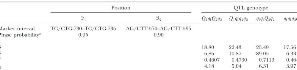
TABLE 1

MLEs of the positions of two QTL, each bracketed by a different marker interval, QTL effects described by growth parameters (a,b,c), and phase probabilities for the QTL located within a marker interval on

linkage group D16 in an interspecific hybrid population of Populus

Position QTL genotype

ᏽ1 ᏽ2 Q1q1Q2q2 Q1q1q2q2 q1q1Q2q2 q1q1q2q2

Marker interval TC/CTG-730–TC/CTG-735 AG/CTT-570–AG/CTT-595

Phase probabilitya _0.95 _0.90

aˆ 18.80 22.43 25.49 17.56

bˆ 6.86 10.87 89.05 6.33

cˆ 0.4607 0.4730 0.7113 0.4648

tI 4.18 5.04 6.31 3.97

a_{Linkage phase here is meant between the uppercase allele of the QTL and the dominant alleles of the flanking markers for}

both intervals.

The tests of the control of other genetic components mapping population (Lin et al.2003). Our functional mapping proposed above was modified to incorporate over the timing of the inflection point can be similarly

made. the uncertainty of the QTL-marker linkage phase into

the likelihood function (appendix).

Detection of QTL with significant epistasis:The statis-A Cstatis-ASE STUDY

tical model built upon a universal logistic growth law (Westet al.2001) is used to map epistatic QTL

responsi-Materials:The power of our statistical model for

map-ble for growth trajectories in poplars. All of the 19 link-ping QTL affecting growth trajectories was

demon-age groups were scanned on a 2-cM scale for the exis-strated by a case study in poplar trees. APopulus deltoides

tence of a pair of QTL at different genomic locations. clone (designated I-69) was used as a female parent to

We have successfully detected a few pairs of genomic mate with an interspecificP. deltoides⫻ P. nigraclone

locations at which two QTL interact to affect stem (designated I-45) as a male parent (Wuet al.1992). A

growth trajectories in poplar. Table 1 and Figure 1 illus-total of 450 1-year-old rooted hybrid seedlings from this

trate an example in which a pair of QTL located at the cross were planted at a spacing of 4⫻ 5 m at a forest

ninth interval [TC/CTG-730, TC/CTG-735] and the farm near Xuchou City, Jiangsu Province, China. The

thirteenth interval [AG/CTT-570, AG/CTT-595] of total stem heights and diameters were measured at the

linkage group D16 (Yinet al.2002) were found to show end of each of the growing seasons for each tree. Two

significant epistatic effects on stem height growth. The parent-specific genetic linkage maps each composed of

uppercase alleles of these two QTL were observed to 19 linkage groups (roughly representing 19 haploid

be in a coupling phase with dominant alleles of their chromosomes in poplar) were constructed from

restric-respective flanking coupling markers. The maximum tion fragment length polymorphism, amplified

frag-(93.1) of the landscape of the log-LR test statistics across ment length polymorphism, and microsatellite markers

the linkage group (Figure 1), greater than the genome-for this hybrid progeny (Yinet al. 2002) and used for

wide threshold at the significance level␣ ⫽0.05 (LRT⫽

the genetic mapping of QTL affecting complex traits

85.6) estimated from permutation tests, justifies the ade-of economical importance in forest trees.

quacy of a two-QTL model incorporating growth curves.

Methods:Yin et al.(2002) used Grattapagliaand

To show the advantages of our functional mapping Sederoff’s (1994) pseudo-test backcross strategy to

con-model, the same data set was analyzed by traditional uni-struct two linkage maps each corresponding to a parent.

variate and multivariate interval mapping approaches. Each testcross marker for these two parent-specific maps

Univariate interval mapping applied to the most differ-is heterozygous in one parent and null in the other.

entiated heights at the oldest age (year 11) measured Because the two parents, I-69 and I-45, are heterozygous,

detected no QTL, whereas multivariate interval map-there is no consistent linkage phase among dominant

ping for three representative ages (years 1, 6, and 11) alleles of different markers on the same linkage group;

suggested a marginal QTL at the significance level␣ ⫽ some are in a coupling phase whereas others are in a

0.10 (results not shown). These results indicate that repulsion linkage phase (Yinet al.2002). Thus, unlike

our functional mapping approach is statistically more QTL mapping in inbred-line crosses, we need to

deter-powerful for detecting QTL from a given mapping pop-mine the correct linkage phase between the QTL and

(7)

Figure1.—The landscape of the log-likelihood ratio for two epistatic QTL across the same linkage group D16 containing 18 markers in poplar (Yinet al. 2002). Two QTL, one located on the ninth marker interval [TC/CTG-730, TC/CTG-735] and the other located on the thirteenth interval [AG/CTT-570, AG/CTT-595], were detected to epistatically determine the overall shape of stem height growth. The plot denotes the critical threshold for the existence of significant QTL. The peak of the landscape corresponding to the genomic locations of two QTL is indicated.

The pseudo-test backcross used here allows for only rameters (Table 1) for four genotypes at two interactive QTL located on linkage group D16 (Figure 2). As de-the significance tests of de-the additive effects of de-the two

QTL and their additive⫻additive epistasis. The thresh- scribed inhypothesis tests, our functional mapping approach can be used to test various genetic hypotheses olds at the␣ ⫽0.05 level for these tests were calculated

by simulation studies with the restrictions 13 and 17, related to the developmental process on the basis of estimated growth parameters. The additive effect of the respectively. By comparing the maximum value of the

LRs from the functional mapping approach with these QTL located on the thirteenth marker interval is sig-nificant throughout the entire growth process mea-thresholds, we found that the additive⫻additive

epista-sis has a significant impact on the overall differences of sured, but its sign is altered when trees develop into age 7–8 years (Figure 2). The QTL located on the eighth growth curve shapes in stem height growth, whereas these

two QTL each display marginally significant effects. marker interval has nonsignificant additive effect on growth, but it interacts significantly with the QTL on the To address a possible violation of the constant

vari-ance assumption in the matrix (8), we incorporate the thirteenth interval. It is not surprising that significant QTL⫻age interactions are detected on height growth TBS model (CarrollandRuppert1984) into our

func-tional mapping framework. Similar results about the given the change of the signs of the additive and additive⫻additive effects (Figure 2).

estimation of QTL positions and effects were obtained

from the TBS-based mapping approach (data not shown). Genetic control over the inflection point:Equation 3 describes the coordinates of the inflection point where Yet, the TBS-based mapping approach provides more

pre-cise estimates of growth curve parameters, with sampling the exponential phase ends and the asymptotic phase begins (Niklas1994). The difference in the coordinates errors reduced by 20–50% compared to those from

un-transformed data. between different genotypes provides important

infor-mation about the genetics and evolution of growth

tra-The dynamic pattern of QTL effect:The growth curves

(8)

Figure2.—The growth curves of four different QTL genotypes drawn using parameter sets (a,b, c) in Table 1 for two QTL detected on the same linkage group D16. The coordinates of the inflection point for each curve are indicated by the horizontal and vertical lines. The differentiation pattern of growth curves beyond the maxi-mum observed age (11 years), af-fected by the QTL, is represented by extended broken curves.

have different ages at the inflection point, this indicates on the basis of clonal replicates. If both parents and that the inflection point is under genetic determination. offspring are cloned, Wu’s model can estimate the en-In our example of poplars, significant additive effect tire additive⫻additive epistatic variance, a partial addi-due to the QTL on the thirteenth marker interval and tive⫻dominant epistatic variance, and a partial domi-significant additive ⫻ additive effect on the timing of nant⫻dominant epistatic variance.

the inflection point are detected. The additive effect of In this article, we present a statistical approach for the QTL on the thirteenth interval delays the occur- _{mapping any QTL that exert various genetic effects on} rence of the inflection point by about 0.4 year, whereas _{growth trajectories based on a genetic linkage map.} the additive⫻additive effect causes the inflection point _{Our approach is unique in that it detects and estimates} to occur 0.8 year earlier (Figure 2). Because the inflec- _{genetic effects due to allelic/nonallelic actions and} in-tion point occurs at a time of maximum growth rate, _{teractions of QTL from physiological and} develop-the genetic control of growth trajectory implies that it _{mental principles of growth. This uniqueness makes our} can be genetically modified to increase a tree’s capacity _{approach advantageous in two aspects and leads us to} to effectively acquire spatial resources. _{construct a conceptual framework of evolutionary}

devel-opmental biology (Arthur2002).

First, we integrate growth equations into a statistical

DISCUSSION _{mapping framework to map developmental QTL that}

guide the trajectories of organ growth and develop-Increasing evidence has emerged for the role of

com-ment. Separate QTL analyses of growth at different time plex genetic architecture in regulating the ontogenetic

points are not powerful to follow the dynamics of QTL development of embryological phenotypes (Cheverud

effects since relationships of growth at different times et al. 1983; Atchley 1984; Atchley and Zhu 1997;

are not considered. Multivariate QTL analysis combin-Vaughn et al. 1999; Carlborg et al. 2003) and,

ulti-ing all time points takes into account these age-depen-mately, shaping the evolutionary process of organismic

dent relationships (Korol et al. 2001), but it quickly form (Wolf et al. 2000). However, traditional genetic

becomes intractable when the number of time points approaches are limited in estimating nonadditive effects.

increases. By fitting the expected genetic values at differ-If epistasis is assumed to be absent, as in most quantitative

ent time points by growth curves (Westet al.2001) and genetic studies,Cockerham’s (1963) model based on a

the residual (co)variance matrix by the AR(1) model mating design provides a nice estimate of the dominant

(Davidian and Giltinan 1995), our approach esti-variance. Wu(1996) extended Cockerham’s

(9)

which thus increases significantly the power to detect age disequilibrium mapping should be integrated within the functional mapping framework. Linkage disequilib-epistasis. Second, because biological principles are

in-rium-based mapping provides a powerful tool for fine-corporated, our approach sheds better light on the

inte-scale mapping of complex traits (Louet al.2003) and, gration of development and epitasis. Our approach

thus, the combination of this mapping strategy with our allows for the understanding of the genetic basis for

functional mapping can gain better insights into the growth and development at the cutting edge of biology

genetic basis of development and evolution. (Raff 2000;Arthur2002). Growth and development

are two different but related biological processes. It We thank two anonymous referees for their constructive comments

is likely that these two processes share some common on this manuscript. This work is partially supported by an Outstanding Young Investigators Award of the National Science Foundation of

genetic mechanisms. By mapping the timing of various

China (30128017), a University of Florida Research Opportunity Fund

developmental events,e.g., the time to first flower, on

(02050259), and a University of South Florida Biodefense grant

the growth curves of QTL genotypes, we can test _{(7222061-12) to R.W. The publication of this manuscript is approved} whether the same growth genes are also involved in as journal series no. R-09586 by the Florida Agricultural Experiment

Station.

regulating reproductive behaviors.

The estimation precision of additive, dominant, and epistatic effects on growth at particular time points,

at time intervals, or during the entire growth process _{LITERATURE CITED} depends on the estimation precision of the parameters

Alberch, P., S. J. Gould, G. F. OsterandD. B. Wake, 1979 Size

describing growth curves. Our earlier studies using a

and shape in ontogeny and phylogeny. Paleobiology5:296–317.

real example have demonstrated that growth parame- Arthur, W., 2002 The emerging conceptual framework of evolu-tionary developmental biology. Nature415:757–764.

ters of different QTL genotypes can be precisely

esti-Atchley, W. R., 1984 Ontogeny, timing of development, and

ge-mated (Maet al.2002;Wuet al.2002, 2004). The sam- _{netic variance-covariance structure. Am. Nat.}_123:_519–540. pling errors of the growth parameters estimated from Atchley, W. R., andJ. Zhu, 1997 Developmental quantitative

genet-ics, conditional epigenetic variability and growth in mice.

Genet-Fisher’s information index are less than one-tenth of

ics147:765–776.

the parameter values when a modest sample size (90) was _{Bertalanffy, V. L}_{., 1957} _{Quantitative laws for metabolism and} used. Moreover, these sampling errors can be reduced if growth. Q. Rev. Biol.32:217–231.

Carlborg, O., S. Kerje, K. Schutz, L. Jacobsson, P. Jensenet al.,

functional mapping is based on the transform-both-sides

2003 A global search reveals epistatic interaction between QTL

model, as advocated byCarrollandRuppert(1984), _{for early growth in the chicken. Genome Res.}_13:_413–421. for relaxing the variance stationarity assumption in the Carroll, R. J., andD. Ruppert, 1984 Power-transformations when

fitting theoretical models to data. J. Am. Stat. Assoc.79:321–328.

AR(1) model. The estimation precision of parameters

Cheverud, J. M., andE. J. Routman, 1995 Epistasis and its

contribu-in the real example is consistent with that from our _{tion to genetic variance components. Genetics}_139:_1455–1461. simulation studies. It is inferred from these results that Cheverud, J. M., J. J. RutledgeandW. R. Atchley, 1983 Quantita-tive genetics of development—genetic correlations among

age-the estimation of age-the genetic architecture of a

quantita-specific trait values and the evolution of ontogeny. Evolution37:

tive trait from our functional mapping approach should _895–905.

be adequately precise, although direct assessments of Churchill, G. A., and R. W. Doerge, 1994 Empirical threshold values for quantitative trait mapping. Genetics138:963–971.

the sampling errors for the gene effect estimation from

Cockerham, C. C., 1963 Estimation of genetic variances, pp. 53–94

our approach are needed. In addition, it is possible to _in_{Statistical Genetics and Plant Breeding}_{, edited by W. D.}_Hanson modify our analysis model to consider nonstationary and H. F. Robinson. Pub. 982, National Academy of

Science-National Research Council, Washington, DC.

variance-covariance structures using structured

antede-Davidian, M., andD. M. Giltinan, 1995 Nonlinear Models for Repeated

pendent models, as proposed byNunez-Anton(1997) _{Measurement Data}_{. Chapman & Hall, London.}

and Nunez-Anton and Zimmerman (2000). Such a Dempster, A. P., N. M. LairdandD. B. Rubin, 1977 Maximum likelihood from incomplete data via EM algorithm. J. R. Stat.

modification can be viewed as an alternative to the

cur-Soc. Ser. B39:1–38.

rent method based on the variance-stationary assump- _{Grattapaglia, D}_{., and}_{R. Sederoff}_{, 1994} _{Genetic linkage maps of}

tion. Eucalyptus grandis andEucalyptus urophyllausing a

pseudo-test-cross: mapping strategy and RAPD markers. Genetics137:1121–

Genetic effects are expressed differentially during

on-1137.

togeny (Rice 2000; Wolf et al. 2000), as also docu- _{Kirkpatrick, M}_{., and}_{N. Heckman}_{, 1989} _{A quantitative genetic model} mented in our case study of poplar trees. Epistasis is for growth, shape, reaction norms, and other infinite-dimensional

characters. J. Math. Biol.27:429–450.

regarded as a force to determine the direction of

organ-Kirkpatrick, M., D. LofsvoldandM. Bulmer, 1990 Analysis of

ismic evolution. This controversial view can now be _{the inheritance, selection and evolution of growth trajectories.} tested and assessed, using this model and implementing Genetics124:979–993.

Kirkpatrick, M., W. G. HillandR. Thompson, 1994 Estimating the

the estimation process of epistasis. From an evolutionary

covariance structure of traits during growth and aging, illustrated

perspective, however, our approach should be modified _{with lactation in dairy cattle. Genet. Res.}_64:_57–69.

to consider population genetic properties of QTL al- Korol, A. B., Y. I. Ronin, A. M. Itskovich, J. PengandE. Nevo, 2001 Enhanced efficiency of quantitative trait loci mapping

leles, QTL genotypes, and the relationship between the

analysis based on multivariate complexes of quantitative traits.

QTL and markers. If a mapping population is con- _Genetics_157:_1789–1803.

Lander, E. S., andD. Botstein, 1989 Mapping Mendelian factors

(10)

link-underlying quantitative traits using RFLP linkage maps. Genetics APPENDIX: ESTIMATION OF QTL PARAMETERS IN A

121:185–199. _{PHASE-UNKNOWN PSEUDO-TEST BACKCROSS}

Lin, M., X.-Y.Lou, M.Changand R. L.Wu, 2003 A general statistical

framework for mapping quantitative trait loci in nonmodel sys- _{Suppose an interval is flanked by two markers,} ᏹ

u

tems: issue for characterizing linkage phases. Genetics165:901–

andᏹu⫹1, whose dominant nonalleles are in a coupling 913.

phase. A putative QTL, ᏽk, on this interval may have Lou, X.-Y., G. Casella, R. C. Littell, M. C. K. Yang, J. A. Johnson

et al., 2003 A haplotype-based algorithm for multilocus linkage _{different phases relative to the marker alleles. Let}_p

kbe

disequilibrium mapping of quantitative trait loci with epistasis.

the probability of an uppercase QTL allele (Qk) to be

Genetics163:1533–1548.

Lynch, M., andB. Walsh, 1998 Genetics and Analysis of Quantitative in a coupling phase with the dominant marker alleles.

Traits. Sinauer, Sunderland, MA. _{Thus, 1}_⫺_p

kis the probability ofQkto be in a repulsion Ma, C. X., G. CasellaandR. L. Wu, 2002 Functional mapping of

phase with the dominant marker alleles. A second QTL,

quantitative trait loci underlying the character process: a

theoreti-cal framework. Genetics161:1751–1762. Ql, that can be located on different marker intervalsNv

Niklas, K. L., 1994 Plant Allometry: The Scaling of Form and Process. _and_N

v⫹1, or on the same marker intervalsMuandMu⫹1, University of Chicago, Chicago.

also has two different QTL-marker phase probabilities,

Nunez-Anton, V., 1997 Longitudinal data analysis: non-stationary

error structures and antedependent models. Appl. Stoch. Models _p_l _{and 1}⫺ _p_l_{. The combination of the two QTL leads} Data Anal.13:279–287.

to four possible (unknown) phase combinations with

Nunez-Anton, V., andD. L. Zimmerman, 2000 Modeling

nonsta-probabilitiespkpl,pk(1⫺pl), (1⫺pk)pl, and (1⫺pk)(1⫺

tionary longitudinal data. Biometrics56:699–705.

Pletcher, S. D., andC. J. Geyer, 1999 The genetic analysis of age- _p_l_{) if the allelic assignment of one QTL is independent} dependent traits: modeling the character process. Genetics153:

of that of the second QTL. The estimation of unknown

825–835.

parameters should be based on a most likely phase

com-Raff, R. A., 2000 Evo-devo: the evolution of a new discipline. Nat.

Rev. Genet.1:74–79. _{bination (determined by} _p_k_and _p_l_{) inferred from the}

Rice, S. H., 1997 The analysis of ontogenetic trajectories: when a

data. The likelihood functions for the four phase

combi-change in size or shape is not heterochrony. Proc. Natl. Acad.

nations are denoted byL11,L12,L21, andL22, respectively. Sci. USA94:907–912.

Rice, S. H., 2000 The evolution of developmental interactions: epis- _{As shown in}_Lin_{et al.}_{(2003), the mixture-likelihood} tasis, canalization and integration, pp. 82–98 inEpistasis and the

function of these four phase combinations can be

writ-Evolutionary Process, edited by J. B.Wolf, E. D.BrodieIII and

M. J.Wade. Oxford University Press, London/New York/Oxford. ten as

Rougvie, A. E., 2001 Control of developmental timing in animals.

Nat. Rev. Genet.2:690–701. _L₍_⍀_,_p

k,pl)⫽pkplL11(⍀)⫹pk(1⫺pl)L12(⍀) Vaughn, T. T., L. S. Pletscher, A. Peripato, K. King-Ellison, E.

Adamset al., 1999 Mapping quantitative trait loci for murine _⫹₍₁_⫺_p

k)plL21(⍀)⫹(1⫺pk)(1⫺pl)L22(⍀),

growth: a closer look at genetic architecture. Genet. Res. 74:

313–322.

where

West, G. B., J. H. BrownandB. J. Enquist, 2001 A general model for ontogenetic growth. Nature413:628–631.

Wolf, J. B., E. D. Brodie, III andM. J. Wade, 2000 Epistasis and the _L

11(⍀)⫽

兿

n

i⫽1

兺

1

jk⫽0

兺

1

jl⫽0 [␲11

ijkjlfijkjlf(y)] , Evolutionary Process. Oxford University Press, London/New York/

Oxford.

Wu, R. L., 1996 Detecting epistatic genetic variance with a clonally

L12(⍀)⫽

兿

n

i⫽1

兺

1

j_k⫽0

兺

1

j_l⫽0

[␲12

ij_kj_lfij_kj_lf(y)] ,

replicated design: models for low- vs. high-order nonallelic inter-action. Theor. Appl. Genet.93:102–109.

Wu, R. L., M. X. WangandM. R. Huang, 1992 Quantitative genetics

L21(⍀)⫽

兿

n

i⫽1

兺

1

j_k⫽0

兺

1

j_l⫽0

[␲21

ij_kj_lfij_kj_lf(y)] ,

of yield breeding for Populus short rotation culture. I. Dynamics of genetic control and selection models of yield traits. Can. J. For. Res.22:175–182.

Wu, R. L., C. X. Ma, M. Chang, R. C. Littell, S. S. Wuet al., 2002 _L₂₂₍⍀₎⫽

兿

n

i⫽1

兺

1

j_k⫽0

兺

1

j_l⫽0

[␲22

ij_kj_lfij_kj_lf(y)] .

A logistic mixture model for detecting major genes governing growth trajectories. Genet. Res.79:235–245.

Wu, R. L., C. X. Ma, M. C. K. Yang, M. Chang, U. Santraet al., _{The probabilities (}␲..

ij_kj_l) of two-QTL genotypes,

condi-2003a Quantitative trait loci for growth in Populus. Genet. Res.

tional upon marker genotypes for progenyi, are derived

81:51–64.

for different phase combinations for the two QTL

lo-Wu, R. L., C.-X. Ma, W. ZhaoandG. Casella, 2003b Functional

mapping of quantitative trait loci underlying growth rates: a para- _{cated on different marker intervals (Table A1) or for} metric model. Physiol. Genomics14:241–249.

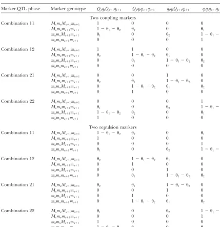
the two QTL on the same interval (Table A2). The EM

Wu, R. L., C. X. Ma, M. Lin, Z. H. WangandG. Casella, 2004

Func-tional mapping of quantitative trait loci underlying growth trajec- algorithm has been implemented to obtain the MLEs

tories using a transform-both-sides logistic model. Biometrics (in _{of vector}_⍀_{and the phase probabilities of the two QTL} press).

pkandpl. In Tables A1 and A2, the conditional probabili-Yin, T. M., X. Y. Zhang, M. R. Huang, M. X. Wang, Q. Zhugeet al.,

2002 Molecular linkage maps of the Populus genome. Genome ties are given for the QTL genotypes bracketed by two

45:541–555. _{coupling dominant markers or repulsion dominant}

markers.

(11)

TABLE A1

Conditional probabilities of QTL genotypes given the marker genotypes forᏹuandᏹuⴙ1 under different marker-QTL linkage phases

Coupling markers Repulsion markers

Marker-QTL Marker-QTL Marker-QTL Marker-QTL

phase 1 phase 2 phase 1 phase 2

Marker genotype Q q qq Q q qq Q q qq Q q qq

MumuMu⫹1mu⫹1 1 0 0 1 1⫺ ␪ ␪ ␪ 1⫺ ␪

Mumumu⫹1mu⫹1 1⫺ ␪ ␪ ␪ 1⫺ ␪ 1 0 0 1

mumuMu⫹1mu⫹1 ␪ 1⫺ ␪ 1⫺ ␪ ␪ 0 1 1 0

mumumu⫹1mu⫹1 0 1 1 0 ␪ 1⫺ ␪ 1⫺ ␪ ␪

␪ ⫽rk1/ru, whereruis the recombination fraction between two markersᏹuandᏹu⫹1andrk1is the recombination fraction between the markerᏹuand the QTLᏽk. Double crossover is ignored.

TABLE A2

Conditional probabilities of the QTL genotypes of two QTL,ᏽkandᏽkⴙ1, bracketed by two markers,ᏹuand

ᏹuⴙ1, conditional on the marker genotypes under different marker-QTL linkage phases

Marker-QTL phase Marker genotype QkqkQk⫹1qk⫹1 Qkqkqk⫹1qk⫹1 qkqkQk⫹1qk⫹1 qkqkqk⫹1qk⫹1

Two coupling markers

Combination 11 MumuMu⫹1mu⫹1 1 0 0 0

Mumumu⫹1mu⫹1 1⫺ ␪1⫺ ␪2 ␪2 0 ␪1

mumuMu⫹1mu⫹1 ␪1 0 ␪2 1⫺ ␪1⫺ ␪2

mumumu⫹1mu⫹1 0 0 0 1

Mumumu⫹1mu⫹1 ␪2 1⫺ ␪1⫺ ␪2 ␪1 0

mumuMu⫹1mu⫹1 0 ␪1 1⫺ ␪1⫺ ␪2 ␪2

mumumu⫹1mu⫹1 0 0 0 0

Mumumu⫹1mu⫹1 ␪2 ␪1 1⫺ ␪1⫺ ␪2 0

mumuMu⫹1mu⫹1 0 1⫺ ␪1⫺ ␪2 ␪1 ␪2

mumumu⫹1mu⫹1 0 1 0 0

Mumumu⫹1mu⫹1 ␪1 0 ␪2 1⫺ ␪1⫺ ␪2

mumuMu⫹1mu⫹1 1⫺ ␪1⫺ ␪2 ␪2 0 ␪1

mumumu⫹1mu⫹1 1 0 0 0

Two repulsion markers

Combination 11 MumuMu⫹1mu⫹1 1⫺ ␪1⫺ ␪2 ␪2 0 ␪1

Mumumu⫹1mu⫹1 1 0 0 0

mumuMu⫹1mu⫹1 0 0 0 1

mumumu⫹1mu⫹1 ␪1 0 ␪2 1⫺ ␪1⫺ ␪2

Combination 12 MumuMu⫹1mu⫹1 ␪2 1⫺ ␪1⫺ ␪2 ␪1 0

Mumumu⫹1mu⫹1 0 1 0 0

mumuMu⫹1mu⫹1 0 0 1 0

mumumu⫹1mu⫹1 0 ␪1 1⫺ ␪1⫺ ␪2 ␪2

Combination 21 MumuMu⫹1mu⫹1 ␪2 ␪1 1⫺ ␪1⫺ ␪2 0

Mumumu⫹1mu⫹1 0 0 1 0

mumuMu⫹1mu⫹1 0 1 0 0

mumumu⫹1mu⫹1 0 1⫺ ␪1⫺ ␪2 ␪1 ␪2

Combination 22 MumuMu⫹1mu⫹1 ␪1 0 ␪2 1⫺ ␪1⫺ ␪2

Mumumu⫹1mu⫹1 0 0 0 1

mumuMu⫹1mu⫹1 1 0 0 0

mumumu⫹1mu⫹1 1⫺ ␪1⫺ ␪2 ␪2 0 ␪1

(12)