A Neural Model for Straight Line Detection in the Human Visual System.

ABSTRACT

JACOB, THEJU ISABELLE. A Neural Model for Straight Line Detection in the Human Visual System. (Under the direction of Wesley Snyder.)

©Copyright 2014 by Theju Isabelle Jacob

A Neural Model for Straight Line Detection in the Human Visual System

by

Theju Isabelle Jacob

A dissertation submitted to the Graduate Faculty of North Carolina State University

in partial fulfillment of the requirements for the Degree of

Doctor of Philosophy

Electrical Engineering

Raleigh, North Carolina

2014

APPROVED BY:

Dror Baron John Franke

Edgar Lobaton Cranos Williams

Wesley Snyder

DEDICATION

ACKNOWLEDGEMENTS

TABLE OF CONTENTS

LIST OF FIGURES . . . vi

Chapter 1 Introduction . . . 1

1.1 Hough Transform . . . 3

Chapter 2 The Visual Cortex. . . 6

2.1 Ganglion Cells, Simple Cells and Complex Cells . . . 7

2.2 Ocular Dominance, Orientation Columns and Receptive Fields . . . 11

2.3 Hough Transform Structure in the Cortex . . . 14

Chapter 3 Hebbian Learning and Self Organizing Networks . . . 16

3.1 Hebbian Learning . . . 18

3.2 Self Organizing Maps . . . 21

Chapter 4 Architecture and Methods . . . 23

4.0.1 Network Architecture . . . 27

4.0.2 Dynamic Network Equations . . . 28

4.1 Results . . . 32

4.1.1 Network Training . . . 32

4.1.2 Performance Comparison . . . 35

4.1.3 Extension to All Orientations . . . 41

4.2 Analysis . . . 48

4.2.1 Maximization of Mutual Information, Under Constraint. . . 49

4.2.2 Experimental Results . . . 51

4.3 Discussion . . . 53

4.3.1 Supervised Learning . . . 55

4.3.2 Self Organizing Maps . . . 57

Chapter 5 Human Experiments . . . 59

5.1 Experiment SetUp . . . 60

5.2 Results . . . 67

Chapter 6 Signal Separation . . . 72

6.1 Separation of Lines . . . 73

6.2 Results and Discussion . . . 75

6.2.1 Comparison with SOM . . . 80

6.2.2 Comparison with Oja’s rule . . . 82

7.1 Conclusion . . . 83 7.2 Future Work . . . 84

LIST OF FIGURES

Figure 1.1 Parameters of a straight line in the Hough space. . . 3

Figure 1.2 Straight lines in Hough space. (Image Source: Nvidia Website) . . . . 4

Figure 2.1 Visual Pathway Structure from [20] . . . 7

Figure 2.2 Cells in Retina from [20] . . . 8

Figure 2.3 Distribution of Rods and Cones in Retina from [1] . . . 8

Figure 2.4 Visual areas from [43] . . . 9

Figure 2.5 Simple and Complex Cells Receptive Fields. . . 10

Figure 2.6 From Hubel [26] - ‘A tilted line segment shining in the visual field of the left eye (shown to the right) may cause this hypothetical pattern of activation of a small area of striate cortex (shown to the left). The activation is confined to a small cortical area, which is long and narrow to reflect the shape of the line; within this area, it is confined to left ocular-dominance columns and to orientation columns representing a two o’clock - eight o’clock tilt.’ . . . 12

Figure 2.7 The first figure shows the drift of receptive fields across 3 mm in cat cortex. Only 4 or 5 receptive fields recorded in the first tenth of each millimeter is shown. The second figure shows the growth in receptive field sizes with increased eccentricity from the fovea, in a macaque monkey, from Hubel [26]. . . 13

Figure 2.8 ‘Ice-Cube model’ of the cortex. The figure shows the division of the cortex into 2 sets of slabs , one for ocular dominance and one for orientation, from Hubel [26]. . . 13

Figure 3.1 Structure of a neuron [7] . . . 16

Figure 3.2 Activity at a Synapse [7] . . . 17

Figure 3.3 Oja’s rule. Effective input at, say node 1, is now x1 - yw1. . . 19

Figure 3.4 Anti-Hebbian Rule leads to decorrelation in output neurons: ∆w12 ∝ -y1y2 . . . 21

Figure 4.1 Simulated cells in the visual pathway . . . 24

Figure 4.2 Orientation sensitive cells at every pixel location in the image plane. Let θ1 correspond to the horizontal line. When two adjacent points along the horizontal direction are excited, their θ1 sensitive cells end up exciting the same accumulator cell. ρ1 represents the distance of the horizontal line from the origin. . . 25

Figure 4.4 Example Architecture . . . 27

Figure 4.5 Winner computation example. Suppose we have an array of neurons. Let the outputs for neurons 1,2, and 6 be 0.1,0.7, and 0.75 respectively. All other neuron outputs are presumed 0. Conventional wisdom would declare neuron 6 as the winner. In our computation, the neuron outputs are multiplied by a Gaussian centered at the neuron locations and added together. The resulting maximum is now located at neuron 2. Neuron 2 is declared the winner. . . 31

Figure 4.6 Resulting network, after training . . . 32

Figure 4.7 Full diagonal line. . . 33

Figure 4.8 Full diagonal line, different position. . . 34

Figure 4.9 Occluded diagonal line. . . 35

Figure 4.10 Horizontal line segment. . . 36

Figure 4.11 Network trained of diagonal line, presented with a clutter. . . 37

Figure 4.12 Separation of peaks example. When two line segments are aligned, only one peak is observed in the accumulator. As the line segments separate, the peaks become more distinct. In the case of addition of noise, more peaks of similar amplitude appears in the accumulator as the standard deviation of the added noise increases. As the peaks become more distinct, the difference between the highest peak in the accumulator and the second highest peak in the accumulator diminishes. 39 Figure 4.13 Variation in angle test images. The angle between the two line seg-ments increases as we move from (a) to (d). . . 40

Figure 4.14 Variation in distance test images. The separation in pixels between the two lines increases from (a) to (d). . . 40

Figure 4.15 Variation in noise test images. The standard deviationσ of the added noise increases from (a) to (d). . . 41

Figure 4.16 Decay of difference in peaks with difference in angle between two line segments for the 4 different implementations. . . 42

Figure 4.17 Decay of difference in peaks with difference in distance between two line segments for the 4 different implementations. The same values were obtained for Accumulator Array Implementation of the Hough Transform and the Conventional Hough Transform, and hence AT plot is omitted. . . 43

Figure 4.18 Decay of difference in peaks with addition of noise for the 4 differ-ent implemdiffer-entations. The same values were obtained for Accumulator Array Implementation of the Hough Transform and the Conventional Hough Transform, and hence AT plot is omitted. . . 44

Figure 4.20 Extension to all orientations by curve estimation. . . 47

Figure 4.21 Network with only intralayer connections. . . 48

Figure 4.22 The training images are the complete shapes in the first column. The second column shows the test images. The third column shows the retrieved images. . . 52

Figure 4.23 Output arrays of the 4 networks, arranged as a pinwheel. . . 54

Figure 4.24 Simple Backpropagation Network . . . 56

Figure 4.25 Radial Basis Function Network . . . 57

Figure 5.1 Focus Screen and Mask Image. . . 61

Figure 5.2 Aligned, Non-Aligned, and Noise Examples. . . 62

Figure 5.3 Aligned and Non-Aligned Contour Examples. . . 63

Figure 5.4 Rotating subpixels to obtain oriented lines. . . 65

Figure 5.5 Plots showing the variation in detection of the lines by the human observers, for all 4 angles when θ,ρ, and noiseσ were varied, in fovea. 68 Figure 5.6 Plots showing the variation in detection of the lines by the human observers, for all 4 angles whenθ,ρ, and noiseσwere varied, in periphery. 69 Figure 5.7 Comparison of fovea and periphery response times. . . 70

Figure 5.8 Results from the contour experiments. . . 71

Figure 6.1 Example Architecture for separation in the orientation space . . . 74

Figure 6.2 Training Images and Resulting Weights, with 4 training lines. . . 77

Figure 6.3 Training Images and Resulting Weights, with 12 training lines. . . 78

Figure 6.4 Weights of 28×28 neurons, arranged in a lattice, after training with MNIST numbers. . . 79

Figure 6.5 Weights of 28×28 neurons, arranged in a lattice, after training with single samples of MNIST numbers 0-7. . . 80

Figure 6.6 Plots showing variation of squared error with increased iterations for a neuron a)within the cluster b)outside the cluster. . . 81

Figure 6.7 Plots showing a) variation of dissimilarity between weights b) squared error between input and weights. . . 81

Chapter 1

Introduction

The human visual system is vastly superior to man made vision systems in its ability to identify objects. Variations in illumination, scale, and position often do not hinder a human observer from identiying a target object. Perception of depth and color further adds to the observer’s ability to distinguish between different targets of interest.

The primary area of the human brain concerned with vision is the visual cortex. Building a model for how the visual cortex identifies different objects is a problem that has attracted much attention over the years. Both top-down [3] and bottom-up [6, 28] approaches have been proposed towards this end. Top-down models start at a high-level representation of the incoming visual input, while bottom-up models start with simple features within the input and then move to more complex features.

discontinuity and noise. A neural model that can learn a Hough Transform-like structure in an unsupervised manner is the main takeaway from this work. Optical illusions like the Poggendorff illusion could potentially find an explanation in the framework of our model.

The main ideas addressed by this thesis can be stated as follows:

ˆ Hypothesis 1:The human visual system may have a Hough Transform like struc-ture for straight line detection in the primary visual cortex.

ˆ Hypothesis 2:A neural network can learn such a Hough Transform like structure.

Hypothesis 1 is addressed in both chapter 2 and chapter 5. Chapter 2 outlines charac-terisitics of the visual cortex that point to the presence of a Hough Transform structure in the cortex, while chapter 5 outlines human experiments that add support to such a computation in the cortex. Hypothesis 2 is addressed primarily in chapter 4.

Models for object recognition based on visual cortex characterisitics like selectivity and scale/position invariance [59, 64, 63] and invariance to lighting conditions [40] have appeared in literature previously. Neural activity models that lead to visual cortex-like characteristics are also found in the literature. For example, learning a sparse code for images as a model for neural activity is discussed in [54, 17]. Predictive coding as an explanation for visual processing in the cortex is discussed in [58]. Information maxi-mization as a goal of sensory coding is discussed in [5, 42, 41]. A self-organizing map architecture capable of extracting features similar to that extracted in the early stages of visual processing is discussed in [34].

x y

θ ρ

(a) A line in Cartesian Space

x y

θ ρ

(b) Mapping from Cartesian Space to Hough Space

Figure 1.1: Parameters of a straight line in the Hough space.

1.1

Hough Transform

The Hough Transform is a popular feature detection technique in computer vision ap-plicatons [11]. The Hough domain, when used to detect straight lines, is characterized by two parameters: 1) the orientation of the line, and 2) the shortest distance from the origin to the line, Fig. 1.1a. The underlying parametric transformation from Cartesian coordinates is represented by the following equation:

ρ=xcos(θ) +ysin(θ) (1.1)

Every point in the Cartesian plane (x,y) gives rise to a sinusoid in the Hough domain Fig. 1.2. The sinusoids from points lying along a line intersect at a single point represent-ing theρ,θ values of the line. A straight line in the Cartesian domain is thus represented by a single point in the Hough domain.

Figure 1.2: Straight lines in Hough space. (Image Source: Nvidia Website)

array A(ρ,θ) with all possible orientations and distances. The orientations usually vary from 0 to π. The distances vary from 0 to the maximum distance possible in the image plane, usually the length of the diagonal of the image. Once the accumulator is in place, we iterate through the pixels in the test image, and for pixels of interest, we compute the

ρ value for every value of θ and increment the corresponding points in the accumulator. Every point lying along a line in the Cartesian domain contributes to a set of points in the accumulator, Fig. 1.1b. The parameters of the line are obtained by looking at the ρ and θ that give the maximum value. An entire line can be thus deduced from a single point in the accumulator array. The transform is insensitive to clutter and partial occlusion, as we rely on a voting process to determine the parameters of the line.

an accumulator in the cortex.

In this thesis, we examine the possibility of the existence of such an accumulator array in the cortex, with neurons or groups of neurons acting as accumulator cells. We address how the cells in the cortex could self organize into accumulator arrays in an unsupervised manner. Starting at the orientation sensitive layer of neurons, we show how the subsequent layers could self organize to detect the location of a given straight line. We borrow from Hebbian Learning and Oja’s rule to do this. Experiments involving human subjects were conducted to add support to our hypothesis.

Chapter 2

The Visual Cortex

The human visual system enables us to process and respond to all kinds of visual stimuli. Various structures along the visual pathway, shown in Fig. 2.1, constitute the visual system. Starting at the retina, neural information travels through the optic nerve to reach the lateral geniculate nucleus (LGN). Information travels further from the LGN to reach the visual cortex, the area of the cerebral cortex responsible for processing of visual information.

The retina itself is a complex structure, with rods and cones acting as photodetectors, and layers of horizontal, bipolar, amacrine, and ganglion cells above them before optic nerve fibres are reached, Fig. 2.2. The fovea is located almost at the center of the retina, representing about 5◦ of visual angle. The highest concentration of cone cells and a near absence of rod cells are found at the fovea, Fig. 2.3. The outer region surrounding the fovea is called perifovea.

Figure 2.1: Visual Pathway Structure from [20]

caused it to have the name ‘striate cortex’. The striate cortex is divided into layers numbered from 1 through 6 based on cell density.

Next considered in this chapter is the architecture and functionality of the visual cortex as described by Hubel [26]. We start with the hierarchial structure of cells found in the visual pathway and cortex and a description of their functionality. We then examine how the cells are grouped across the cortex, and how their organization could imply an architecture suitable for Hough Transform computation.

2.1

Ganglion Cells, Simple Cells and Complex Cells

Figure 2.2: Cells in Retina from [20]

Figure 2.4: Visual areas from [43]

center of their receptive fields, and low responses when light falls outside the center of their receptive fields. The opposite is true for off-center cells. Their receptive fields hence approximate a second order derivative function. Both are found equally across the retina, and appear to be intermixed. The receptive fields of these cells are circularly symmetric, and the orientation of the stimulus does not matter. The receptive fields of cells in the LGN have the same structure as the retinal ganglion cells that feed into them. The cells in the first stage of the visual cortex respond like the cells in the LGN as well.

in the output of the cell.

Complex cells, which make up about three quarters of cells in the visual cortex, respond only to specifically oriented inputs. They may or may not respond to stationary input, but if they do respond to stationary input, they respond irrespective of where the input is located in the receptive field. That is, they do not appear to have the excitation and inhibition regions as were observed in cells in previous stages. Complex cells also have larger receptive fields than simple cells, Fig. 2.5b.

(a) Simple cell receptive fields con-structed from on-center cells [26].

(b) Complex cell receptive fields con-structed from simple cells [26].

Figure 2.5: Simple and Complex Cells Receptive Fields.

A typical orientation-selective cell does not respond at all when the line is oriented 90 degrees to the optimal. All orientations are about equally represented in the cortex.

Orientation sensitive cells can be modeled using Gabor filters [9]. Gabor filters are usually used for detection of edges in images. The following equations represent the operation of a Gabor filter, where xand y refers to the coordinates in thex-y plane and

x0 =xcos(θ) +ysin(θ)

y0 =−xsin(θ) +ycos(θ)

gf(x, y, θ) = exp(−(x

0₎2_+γ2_(y0₎2 2σ2 )cos(

2πx0 λ )

(2.1)

2.2

Ocular Dominance, Orientation Columns and

Re-ceptive Fields

On inserting a probe perpendicular to the cortical surface, Hubel and Wiesel found that cell after cell favored the same eye - that is, the left eye or right eye. On inserting a probe parallel to the surface, the dominance of the left eye or the right eye was found to alternate back and forth. The reason why this phenomena occurs is thought to be found in the way the geniculate fibers (which are monocular) terminate in the cortex. A complete cycle of right eye and left eye dominance is found once every millimeter.

Similar to ocular dominance, orientation preference was found to remain constant in vertical penetration of the cortex. On inserting the probe parallel to the surface of the cortex, the orientation shifted by 10 degrees clockwise or counterclockwise for every 0.05 mm advance. A complete 180 degree shift was observed once every millimeter. These observations allowed Hubel and Wiesel to define a local coordinate system on the visual cortex, Fig. 2.6. Ocular dominance and orientation groupings of cells appeared not to influence each other .

Figure 2.6: From Hubel [26] - ‘A tilted line segment shining in the visual field of the left eye (shown to the right) may cause this hypothetical pattern of activation of a small area of striate cortex (shown to the left). The activation is confined to a small cortical area, which is long and narrow to reflect the shape of the line; within this area, it is confined to left ocular-dominance columns and to orientation columns representing a two o’clock - eight o’clock tilt.’

3, 4 etc.) under some point on the cortex. In a given layer, the aggregate receptive field could vary from a few minutes in the foveal region to a few degrees in the far periphery. On moving the probe parallel to the cortical surface, a steady drift in position across the visual field was observed, Fig. 2.7. The rate of movement was observed to be constant relative to the size of the receptive fields. Approximately 2 mm of movement would take one entirely out of one part of the visual field, onto the next.

Figure 2.7: The first figure shows the drift of receptive fields across 3 mm in cat cortex. Only 4 or 5 receptive fields recorded in the first tenth of each millimeter is shown. The second figure shows the growth in receptive field sizes with increased eccentricity from the fovea, in a macaque monkey, from Hubel [26].

2.3

Hough Transform Structure in the Cortex

Suppose (ρ,θ) parameterization is used. To characterize straight lines, we need 2 factors -1) Orientation of the line, and 2) Position of the line in the visual field. In Hough Trans-form space, every curve belonging to a straight line passes through a single point whose co-ordinates give us the orientation and position of the line. If we use accumulators to implement the Hough Transform [66], we have an array with, say, orientation information in degrees along the columns and the position information in terms of distance from a chosen origin along the rows. On reviewing what we know of the visual cortex structure, we can speculate that the on-center/off-center cells act as units of addition/accumulation. When any such cell is stimulated by the presence of a point in the visual field, it con-veys that information to the simple cell it is connected to, effectively doing a +1 to that particular simple cell. As more on-center cells connected to a simple cell is activated, we detect a line of a particular orientation.

The simple cells are our gradient detector units, as they are specific in the orientation they respond to. As a group of simple cells contribute to the complex cell, and the complex cell receptive fields cover only a certain portion of the visual field, we speculate that the complex cells act as the location detector for the line. That is, we can determine the location of the line by looking at the receptive field location of the complex cell that responds to that particular line.

Chapter 3

Hebbian Learning and Self

Organizing Networks

In this chapter, we briefly examine the structure and signalling operations of a neuron and learn how two neurons interact. We then look at the learning rules which have been proposed to model such interactions between groups of neurons. All images in this chapter are from [7] unless otherwise stated.

The structure of a neuron is shown in Fig. 3.1. The neuron consists of a cell body, dendrites, and an axon. The dendrites and the axon are structures arising from the cell body which are used to communicate with other neurons. Signalling happens in a neuron by variation of its membrane potential. The inside of a neuron cell membrane is about -70 mV relative to the outside. [Na+] and [Cl-] are higher outside, while [K+] is higher inside. The cell membrane is a lipid bilayer impermeable to these charged ions, but with embedded ionic channels to allow the ions to flow in or out. Ionic pumps along the membrane strive to maintain the equilibrium potential of -70 mV. For further details of their operations, refer [10, 67, 2].

Interactions between neurons happen at the junction where axons from one neuron interact with dendrites or the cell body of another neuron. Such junctions are called synapses. Synapses can be excitatory or inhibitory. An incoming spike along the axon

of a neuron, called ‘presynaptic cell’, causes the release of neurotransmitters into the synapse. The neurotransmitters bind to the ion channel receptors of the dendrites of the second neuron, called the ‘postsynaptic cell’. The ion channels in the second neuron then open, causing either depolarization or hyperpolarization, depending on whether the synapse was excitatory or inhibitory, Fig. 3.2.

The Hodgkin-Huxley equations are popularly used to mathematically describe the effect of an incoming spike on a neuron. Hodgkin and Huxley models the neuron as a RC circuit [67]. Other models like the Integrate and Fire model and its variations are also used to describe neuronal activity. The neuron models found in artificial neural network literature can be derived from the biological neuron models after making a number of simplifying assumptions.

3.1

Hebbian Learning

Neurons learn by means ofsynaptic plasticity. Synaptic plasticity is the ability of synapses to strengthen or weaken over time. A basic mechanism for modification of synaptic strengths was given by Hebb in his seminal work [24]. He postulated that if a presy-naptic cell repeatedly and persistently stimulated a postsypresy-naptic cell, it would lead to an increase the efficacy of the synapse between the two cells.

Hebbian learning as defined for linear neurons can be formalized as follows: Suppose we have a neuron withN inputs. If y represents the output of the neuron and wirepresents

x1

x2

x3

y w1

w2

w3

Figure 3.3: Oja’s rule. Effective input at, say node 1, is now x1 - yw1.

y = P

iwixi

During training, various input samples are presented to the neuron. If the output of the neuron is high when a particular input is on, the weight between that input and the neuron is strengthened. The following equation is used for weight update, where αis the learning parameter:

∆wi = αyxi

In the absence of constraints in Hebbian learning, the weights tend to grow without bounds. Decay terms were hence introduced in the learning rule itself [44, 69, 47, 35, 33]. For a detailed treatment of the type of constraints in Hebbian learning, see [45].

Oja’s rule [47] for a single neuron introduces a decay term in the weight update rule, derived by normalizing the incoming weights to a neuron to have an Euclidean norm of unity. Oja’s rule ends up extracting the largest principal component of the data. The weight update rule now looks like:

Oja’s Subspace Algorithm [48] extended the above rule to N output neurons. The weights then do not necessarily converge to the actual Principal Components of the input space, but they do converge to an orthonormal basis of the Principal Component Space. The weight update rule for the weight wij between output neuron yi and input

neuron xj now looks like:

∆wij = α(yixj - yiP_kwkjyk)

Asymmetry was introduced to the Subspace Algorithm in the form of a parameter θ

in order to force the weights to converge to the Principal Components [49, 52, 53]. The weight update equation now looks like:

∆wij =α(yixj - θiyi

P

kwkjyk)

Withθ1< θ2 < θ3 · · ·, the weight vectors will converge to the principal eigenvectors in the order of their eigenvalues. The value of θi should be close to 1 to ensure convergence.

Nonlinear extensions to the above rule and its analysis can be found in [51] and [50]. A derivation of the nonlinear PCA rule from a error minimization and feature extraction approach is given in [32].

Sanger developed the Generalized Hebbian Algorithm [61] which also found the Prin-cipal Components of the input space, but introduced asymmetry in the feedback term. The weight update equations are then:

∆wij = α(yixj - yiPi_k=1wkjyk)

x1

x2

x3

y1

y2

w12 = w21

Figure 3.4: Anti-Hebbian Rule leads to decorrelation in output neurons: ∆w12 ∝ -y1y2

for feature extraction [16]. The simplest weight update rule for the weight wij between

output neuron yi and input neuron yj would then be:

∆wij = -αyjyi

3.2

Self Organizing Maps

Competitive learning, orwinner take all algorithms, are another group of algorithms that

model relationships between neurons in the same layer. They form a powerful tool for feature discovery and leads to self organization of networks [60, 44, 69, 35]. They rely on competition, cooperation and synaptic adaptation amongst the neurons in the network [23]. Consider Kohonen’s Self Organizing Mapor SOM: The neuron declared as the win-ner i∗ in any iteration is the one whose weights wj resemble the input x at that iteration.

That is:

i∗ = argmin

j

(kx - wjk)

hj= exp(

−ki∗−jk2

2σ2 )

.

When the weights associated with any particular neuron are updated, the neighbour-hood function’s value at that particular neuron’s location is multiplied with the learning parameter:

∆wj =αhj(x - wj)

Chapter 4

Architecture and Methods

The key ideas addressed by this thesis can be stated as follows:

ˆ Hypothesis 1:The human visual system may have an accumulator-array structure for detection of straight lines in the primary visual cortex.

ˆ Hypothesis 2: The accumulator-array structure can be learned.

Hypothesis 1 was addressed in Section 2.3. The proposed network of neurons that leads to an accumulator-like computation in the cortex is described later in this section. The architecture and the learning rules detailed next lead to ρ-θ parameterization of straight lines as described in Chapter 1.

input image

orientation sensitive

cells

position sensitive

cells visual pathway

Figure 4.1: Simulated cells in the visual pathway

as shown in Fig. 4.1.

Suppose we are interested in 4 of all the possible orientations - θ1, θ2, θ3,θ4. When a point in the visual field is illuminated, all 4 of the orientation sensitive cells at the point receive stimulus. They feed into all of the corresponding cells in the accumulator array. When a line of a given orientation falls in the visual field, a collinear set of points gets excited. The cells in the corresponding orientation column responds strongly. As points along a line of given orientation have the same ρ, they all excite a single accumulator cell very strongly. This can be represented by the following equation whereA(ρ,θ) is the accumulator cell, and N is the number of points along the line:

A(ρ, θ) =

N

X

i=1

image plane orientation sensitive cells

accumulator cells θ1,ρ1 θ2,ρ2

θ1 θ2 θ3 θ4 θ1 θ2 θ3 θ4

Figure 4.2: Orientation sensitive cells at every pixel location in the image plane. Let

θ1 correspond to the horizontal line. When two adjacent points along the horizontal direction are excited, their θ1 sensitive cells end up exciting the same accumulator cell.

x y

θ θ1 θ2 θ3 θ4

ρ

Figure 4.3: Connections between pixels in the image plane and the cells in the accumu-lator. For clarity, only the connections which give rise to the two strongest responses in the accumulator array are shown.

This is demonstrated in Fig. 4.2 for the case where θ1 corresponds to the horizontal line.

The case with multiple lines is demonstrated in Fig. 4.3. Theθ2 receptors of the points lying along the red line feed into a single cell in the θ2 column. The θ1 receptors of the points lying along the blue line feed into a single cell in theθ1 column. The point at the junction of the two lines feed into both columns.

The network described clearly lead to an accumulator array. The important question is: can such a network be learned? We next show how the neurons that receive their inputs from the orientation sensitive cells could learn the position of the given line. That is, we are interested in learning the connections from the θ sensitive cells to the correponding

y1 x1 y2 x2 y3 x3 y4 x4 z1 z2 input samples position output input layer output layer ¯ w11

w12 =w21

ˆ

w12 = ˆw21

Figure 4.4: Example Architecture

clutter.

4.0.1

Network Architecture

The network of interest consists of two groups of neurons, both arranged in 2-dimensional lattices - let us call them the input array and the output array. An example is shown in Fig. 4.4. The input array neurons receive signals from the input image, and also from neighboring neurons within the same array. These cells represent the orientation-sensitive simple cells in the cortex.

input array as well as to neighboring neurons in the same array. They represent what will be the position sensitive cells, after training. The neuron with the maximum output will indicate the location of the input in the visual field, and will act as the input to deeper arrays in the cortex. For example, after training, when a test image with a horizontal line at the second row is given as input to the network, the maximum in the output array will occur at the neuron at the center of the second row. Assuming the origin to lie in the center of the output array, the neuron with the maximum indicates the shortest distance from the origin, which is alsoρ.

The intra-array connection strengths are assumed to be symmetric - that is, the strength of the connection going from neuron atob within the same array is assumed to be the same as that going from neuron bto a . No self feedback is assumed.

The intra-array neighborhood of a neuron is defined as the group of neurons within a specified distance, when the neurons are arranged in a 2-dimensional lattice. Similarly, for inter-array connections, the neighborhood is the group of neurons from the input array that connect to an output neuron, when the input and output lattices are placed center to center and an equal number of input neurons are assumed to connect to every output neurons.

We build a network as shown in Fig. 4.4 for every orientation under consideration. After training, the output array of any given network will indicate the position of a line of corresponding orientation. This leads to an accumulator array like structure.

4.0.2

Dynamic Network Equations

between neurons in the same array.

Let x denote the external input, y denote the input neuron array and z denote the output neuron array. The output at each array is computed as follows:

yi(t) = f(

X

j

wijyj(t−∆t) +xi)

zi(t) = f(

X

j

ˆ

wijzj(t−∆t) +

X

j

¯

wijyi)

(4.2)

In (4.2), f refers to a smooth thresholding function like the sigmoid or the hyperbolic tangent. ∆t indicates increments in time. The neuron outputs decay as follows, where

decay < 1:

yi(t+ ∆t) =decay∗yi(t)

zi(t+ ∆t) =decay∗zi(t)

(4.3)

The decay parameter was chosen empirically.

While updating weights, the aim is to strengthen the connections between neurons that fire together, while resulting in a stable network. For weights between the input and output arrays, Oja’s rule is used. For neurons in the same array, the weights increase if the outputs of the neurons correlate, but with a restraining factor, β.

The weights between the input and output array are updated as follows, where α is the learning parameter:

¯

wij = ¯wij +αzi(t)(yj(t)−zi(t) ¯wij) (4.4)

The weights between the neurons in the output array are updated as follows, where

ˆ

wij = ˆwij +α(zi(t)zj(t)−βwˆji) (4.5)

The weights between neurons in the input array are similarly updated. The learning parameter decreases with time in an exponential manner. That is, ifαo denotes the initial

value of the learning parameter:

α(t) = αoexp(−

t

τ) (4.6)

The input array is assumed to have the same size as that of the incoming input signal. The output array has a reduced size along one dimension - if the array is of size n ×

m, m << n. This is noticeable in Fig. 4.7-4.11. The reduced size for the output array is justified as follows: Suppose an output array the same size as that of the input array is used. After training with horizontal lines, for example, it can be found that only a few neurons in each row of the output array are needed to represent the input samples. We can hence do away with some of the columns in the output array, thereby reducing the dimension of the output array.

Such a two-array network was built for every orientation of interest, Fig. 4.6. Each network was trained separately. The training samples consist of lines of the chosen ori-entation, located at all possible locations in the input image. The first array learned to become orientation sensitive, by means of its intra-array connections, resulting in the θ

value. The second array learned to denote the ρ for the corresponding θ from the first array. Taken together, this results in the ρ-θ architecture described previously.

cause some excitation in the other.

0 2 4 6 8

0 0.1 0.2 0.3

0.1

0.7 0.75

sum

0 2 4 6 8

0.1 0.2

0.3 winner

Figure 4.5: Winner computation example. Suppose we have an array of neurons. Let the outputs for neurons 1,2, and 6 be 0.1,0.7, and 0.75 respectively. All other neuron outputs are presumed 0. Conventional wisdom would declare neuron 6 as the winner. In our computation, the neuron outputs are multiplied by a Gaussian centered at the neuron locations and added together. The resulting maximum is now located at neuron 2. Neuron 2 is declared the winner.

After training, the networks were tested using images of lines as well as line segments under various conditions. The peak point or the winning neuron in the output array was determined as follows: every neuron output is multiplied by a two dimensional Gaussian function, and are then summed together. The neuron located at the location of the maximum value is declared the winner, see Fig. 4.5. The winning index in the output array i∗ is determined by:

gi(t) =

X

j

zj(t)˜rij(t)

i∗(t) = argmax

i

(gi(t))

input image

input layer

output layer

θ1

θ2

θ3

θ4

ρ, θ1

ρ, θ2

ρ, θ3

ρ, θ4

Figure 4.6: Resulting network, after training

The ˜rij term represents a 2 dimensional Gaussian neighborhood. This new winning

neighborhood approach leads to more robust results when compared to the conventional approach of declaring the neuron with maximum output as winner.

4.1

Results

4.1.1

Network Training

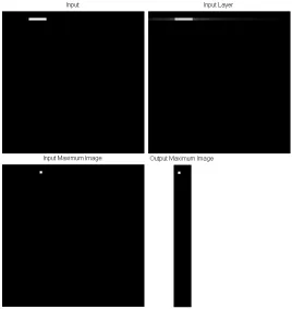
Figure 4.7: Full diagonal line.

images with lines of given orientation located at all posible positions, one line in any given input. The network was trained with the images chosen at random, one array at a time -that is, the input array training was completed before the output array was started. The number of iterations were to the order of about 5000 for every array. The choice of the number of iterations was driven by the rate of decay of the learning parameter, equation (4.6) - once the learning parameter reached a point where the neurons had little effect on each other, training was stopped.

Figure 4.8: Full diagonal line, different position.

the maximum in the output array at the row corresponding to the line. In Fig. 4.9, the same diagonal line, but partially occluded, was given as the input. The input array filled up the occluded portion. The maximum in the input array is now shifted as the input line is incomplete. However, we continue to obtain the same maximum in the output array as the full line, because the output array managed to identify the full line from the segments. In Fig. 4.8, we see a shifted diagonal line. The input array values, as well as the positions of maximum values in the input array and output are shifted as well.

Figure 4.9: Occluded diagonal line.

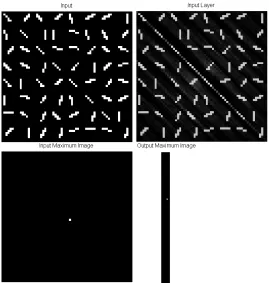
Fig. 4.11 are the results obtained when a network trained with diagonal lines was presented with an image with clutter. The input layer spread out all of the line segments along the diagonal direction. As there were aligned diagonal line segments along the origin, the maximal output corresponded to a diagonal line along the origin.

4.1.2

Performance Comparison

Next compared are the results from 3 different implementations of the Hough Transform, and the neural network trained on straight lines. The 3 implementations of the Hough Transform are

Figure 4.10: Horizontal line segment.

2. The Accumulator Array implementation of the Hough Transform (AT) [see Algo-rithm 2]

3. A Hough Transform implementation using Gabor Filters (GT) [see Algorithm 3]

CT and AT have been discussed already - the only difference between them is that, in AT, the connections from the image pixels to the accumulator array are precomputed and weighted in order to simulate the behaviour of neurons.

Figure 4.11: Network trained of diagonal line, presented with a clutter.

Algorithm 1 Conventional Hough Transform, for an Image I of size M × N. for θ= 0 to π do

for x= 1 to Mdo for y= 1 toN do

ρ=xcos(θ) +ysin(θ)

A(ρ, θ) = A(ρ, θ) + I(x,y) end for

end for end for

x0 =xcos(θ) +ysin(θ)

y0 =−xsin(θ) +ycos(θ)

gf(x, y, θ) = exp(−(x

0₎2_+γ2_(y0₎2 2σ2 ) cos(

2πx0 λ )

Algorithm 2 Accumulator Hough Transform, for an Image I of size M × N. for θo = 0 to π do

for x= 1 to Mdo for y= 1 toN do

ρo=xcos(θo) +ysin(θo)

for ρi =ρo−3 to ρo+ 3 do

for θi =θo−3 to θo+ 3 do

A(ρi, θi) = A(ρi, θi) + I(x,y) e−((ρi−ρo)

2_+(θ

i−θo)2) end for

end for end for end for end for

Algorithm 3 Gabor Filter Hough Transform, for an Image I of size M × N. for θ= 0 to π do

for x= 1 to Mdo for y= 1 toN do

ρ=xcos(θ) +ysin(θ)

A(ρ, θ) = A(ρ, θ) + I(x,y) gf(x, y, θ) end for

end for end for

The value from the Gabor filter is then used to increment the corresponding cell in the accumulator array. The following values were used in (4.8): σ = 1,γ =1, λ =4.

In all three implementations of the Hough Transform, sampling interval for θ is 15◦, while for the neural network, it is 45◦. All possible ρ values are covered.

Three conditions are tested:

1) Difference in θ 2) Difference in ρ, and 3) Presence of Noise.

0 2 4 6 8 0

0.1 0.2

0.3 single peak

separation of lines

0 2 4 6 8

0 0.1 0.2

0.3 peak1 peak2

Figure 4.12: Separation of peaks example. When two line segments are aligned, only one peak is observed in the accumulator. As the line segments separate, the peaks become more distinct. In the case of addition of noise, more peaks of similar amplitude appears in the accumulator as the standard deviation of the added noise increases. As the peaks become more distinct, the difference between the highest peak in the accumulator and the second highest peak in the accumulator diminishes.

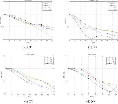
For testing the difference in θ, we presented images with two line segments, which were collinear at first. The angle between the two line segments were gradually increased. The difference between the highest and the second highest value in the accumulator was plotted. The difference gradually decreased as the lines became more distinct. Fig. 4.16 show the results. The curves follow a similar trend in all cases.

For testing the difference in ρ, we presented images with two line segments, which were aligned at first. One of the line segments was then displaced. The difference between the highest and the second highest value in the accumulator was plotted. The difference gradually decreased as the lines became more distinct. Fig. 4.17 show the results.

(a) 0◦ (b) 15◦

(c) 30◦ (d) 45◦

Figure 4.13: Variation in angle test images. The angle between the two line segments increases as we move from (a) to (d).

(a) 0 pixels (b) 4 pixels

(c) 6 pixels (d) 10 pix-els

(a) σ= 0 (b)σ= 10

(c)σ= 20 (d)σ= 30

Figure 4.15: Variation in noise test images. The standard deviationσ of the added noise increases from (a) to (d).

the noise was increased. As standard deviation was increased from zero, multiple peaks appeared in the accumulator array for all 4 implementations. The results are shown in Fig. 4.18.

Another question to ask is: when does the accumulator claim that there are 2 lines present, instead of 1? What is the breakpoint after which the second highest peak is at least 75% of the highest peak? Plots with these results are shown for CT and GT Fig. 5.2.

4.1.3

Extension to All Orientations

The architecture outlined can be extended to detect other orientations in two ways

-1. Build and train separate networks for lines of separate orientations, or

2. Estimate the “actual” orientation from the peak outputs of the 4 networks already trained.

(a) CT (b) AT

(c) GT (d) NN

(a) CT (b) AT

(c) GT (d) NN

(a) CT (b) AT

(c) GT (d) NN

(a) CT angle (b) GT angle

(c) CT distance (d) GT distance

(e) CT noise (f) GT noise

separately with lines of the following orientations - 0◦, 45◦, 90◦, and 135◦. The outputs of these networks (after training), for each of the 4 orientations, are then considered.

As expected, each network responds maximally to the orientation with which it was trained, Fig. 4.20a. For example, after training, the 0◦ network responds maximally to a horizontal line, while the 90◦ responds minimally to it. A curve is then fitted to pass through the output values of each of the networks, for each of the orientations, using a standard interpolation algorithm. We used an inbuilt MATLAB interpolation algorithm using the Fast Fourier Transform (FFT). The points are transformed to the Fourier domain using FFT, and then transformed back to obtain more points.

Four curves are obtained after the interpolation process. These 4 curves are all cen-tered, Fig. 4.20b and averaged, Fig. 4.20c, to obtain a single curve which captures the variation in outputs from each of the trained networks. Let this curve be called the “out-put” curve, f(θ), with a peak at θ = 90◦. The curve is then shifted to peak at θ = 0◦.

A test line (of any orientation) is then presented to the 4 networks, and their outputs are considered. Once again, a curve is fitted through the 4 outputs. Let the resulting curve be g(θ), whereθ varies from 0 to π. The “output” curve is made to slide over the resulting cuve (much like in a convolution), and the square of the error between both curves are computed. The angle corresponding to the location of minimum error is then declared as the angle of the test line:

φ∗ = argmin

φ

(X

θ

(a) Curves obtained for the four angles. (b) The four curves centered.

(c) Single curve after averaging.

x1 y1

x2 y2

x3 y3

x4 y4

input samples

output samples

v12=v21

Figure 4.21: Network with only intralayer connections.

4.2

Analysis

In this section, a mathematical analysis of the network in Fig. 4.4 is provided. As dis-cussed before, connections are present between neurons in the same layer as well as between neurons in different layers. The connections between neurons in different layers are governed by Oja’s rule, as seen in equation (4.4). Oja’s rule has been analyzed in detail in literature previously, see Chapter 3.

4.2.1

Maximization of Mutual Information, Under Constraint.

y=x+Vy (4.10)

It has to be noted that V is symmetric and that Tr(V) = 0. That is, there is no self feedback in the output neurons and that the connections are symmetric. The above can be rewritten as follows, where W represents a weight matrix between input and output:

y= (I−V)−1x=Wx (4.11)

Wcan be thought of as a mapping fromx∈_RN _toy∈

RN, whereN is the dimension

of the vector space.

Consider the case where the presented inputs have a multivariate Gaussian probability density function with zero mean. If N is the dimension of xand P

x = E(xx

T_{) denotes}

the covariance matrix of x, the we can write:

P(x) = 1

(2π)N/2_(|P x|1/2)

exp(−1

2x

TX−1

x x) (4.12)

Now consider the output unit y1, element of the vector y. We can write:

y1 =x1+

N

X

i=2

v1iyi (4.13)

I(y1, y2) = E

ln

P(y1, y2)

P(y1)P(y2)

(4.14)

E represents the expectation operator. With the given probability density function

for the inputs, with column vector y12 = [y1 y2]T and

P

y1,y2 the covariance submatrix

for y1 and y2, we can write:

P(y1, y2) =

1 2π(|P

y1,y2|

1/2₎exp

−1 2y T 12 X−1

y1,y2

y12

P(y1) = 1 (2πσ2

y1)

1/2 exp

−1 2 y2 1 σ2 y1

P(y2) = 1 (2πσ2

y2)

1/2 exp

−1

2

y₂2 σ2

y2

(4.15)

Consider the case where all of the connecting weights to y1 are constrained to have a norm of 1. That is,

q

PN

i=2v12i = 1. Using the principle of Lagrange multipliers, we can

construct the following cost function:

E =I(y1, y2)−λ

  v u u t N X i=2 v2 1i−1



 (4.16)

Next, we differentiate the cost function with respect to the weight betweeny1 and y2,

v12. We use the following results for the same:

∂y1

∂v12 =y2,

∂y2

∂v12

=y1,

∂σ2

y1

∂v12

= 2σ_y2_1,y2,∂σ

2

y2

∂v12

= 2σ_y2_1,y2,∂σ

2

y1,y2

∂v12

=σ2_y1 +σ2_y2 (4.17)

In the above equation,σ2

y1 is the variance ofy1 and σ

2

y2 is the variance ofy2 and σ

2

y1,y2

is the covariance of y1 and y2.

∂E

∂v12

=y1y2( 1 σ2 y1 + 1 σ2 y2 ) + σ 2

y1,y2

σ2

y1

(1− y

2 1 σ2 y1 ) + σ 2

y1,y2

σ2

y2

(1− y

2 2

σ2

y2

)−λv12 (4.18)

For slowly varying weight v12, the average of the second and the third term vanishes. So we are left with the term proportional toy1y2and the term arising from the constraint. If we were to do a gradient ascent on the weight, we would end up with the weight update equation:

∆v12=α(y1y2−λv12) (4.19) This is the same as equation (4.5).

4.2.2

Experimental Results

A single layer neural network with the architecture and weight update equations as discussed in the previous section was trained. The training samples were the images of shapes shown in first column of Fig. 4.22. The starting value for αwas 0.1. The value for

4.3

Discussion

We have seen how unsupervised neural networks can construct accumulators with the help of a few learning rules. Once the accumulator structure is in place, the network can rapidly identify any given line by its orientation and position. The network can identify the line even in the presence of occlusion and moderate amounts of noise, by looking at the winning cell which has the maximum output value in the presence of a given input.

The network is also comparable to the different implementations of the Hough Trans-form in terms of the ability to distinguish separate lines. When the angle between two line segments was increased, the difference between accumulator peaks gradually decreased to zero, thereby identifying the lines as separate - the curve of the graphs obtained were similar for the network and various Hough Transform implementations. The same trend was observerd when the distance between two line segments was increased, as well as when noise was added to the test images.

The network can be further extended by including more arrays to enable it to identify curves or more complex shapes. This hierarchy of accumulator cells would result in having a cell or group of cells respond maximally to a frequently encountered input, leading to a sparse representation of input data. Experimental results supporting this idea for visual objects have appeared in literature [37, 57].

Log-Polar Transform:

0◦

90◦ 45◦ 135◦

Figure 4.23: Output arrays of the 4 networks, arranged as a pinwheel.

of cells. The cell or group of cells with the maximum value would indicate the position, or the distance of the line from the origin, ρ.

Now consider a particular point p in the input image. Let the point be at a distance

d from the origin. Any line which passes through p will have a ρ which is less than or equal tod, i.e., ρ ≤d. Since p will contribute to the accumulator array every time a line passes through p, the cells excited by pointp will indicate lines withρfrom 0 tod. That is, p should excite a total of d number of cells in the accumulator array. Since a point closer to the origin will have adthat is smaller than that of a point which is farther away from the origin, this in turn implies that a point closer to the origin will excite fewer cells when compared to a point farther away from the origin. Hence all points which lie at the same distance from the origin will excite the same number of cells in the accumulator. This is in agreement with the log polar transform idea.

Pin-wheel Model:

ori-entation sensitive cells are arranged in a pin-wheel like fashion around a center. While traversing the pin-wheel structure, either in clockwise or in anti-clockwise direction, the orientations to which the encountered cells are sensitive to, vary smoothly.

The network presented in this chapter fits into this construct as well. Consider the second array of the 4 trained networks. When overlapped with centers coinciding, they present a pin-wheel like structure, see Fig. 4.23. The orientations to which the cells are sensitive to vary smoothly in both clockwise and counter-clockwise direction in the structure.

Next, some of the other neural network implementations that were explored are out-lined.

4.3.1

Supervised Learning

Supervised learning techniques were initially investigated for learning the accumulator array like structure. The supervised learning techniques tried were: 1)Backpropagation network 2)Radial Basis Function network.

1) Backpropagation Network: Consider the network in Fig. 4.24. The input image, NxN in dimension, is fully connected to the output layer, Nx1 in dimension. The weight matrix is NxNxN in dimension. The inputs and expected outputs are defined as following: Suppose only horizontal lines are considered. Since the input image is NxN, there are a total of N distinct horizontal lines. For each of those N horizontal lines, a particular cell from the Nx1 output layer should turn on, while the rest of the cells remain in off position. For example, if there is a line in row 1 in the input image, cell 1 from the output layer would output 1, while the rest of the cells would output 0.

N=8, with 15000 iterations, the network learned to output the correct cell, for each of the horizontal lines. For N=16, with a learning parameter little higher than that for N=8, the network learned the correct output, with iterations close to 25000. For N=32, even with different learning parameters and iterations as high as 100,000, the network showed only very little reduction in its error, and the complexity made such type of learning infeasible. So the number of input samples were increased to include vertical, diagonal, and anti-diagonal lines. The network was trained to give zero output if any line other than a horizontal line appeared. The network learned the correct output for N=32 as well N=64, for iterations close to 50000.

Figure 4.24: Simple Backpropagation Network

2) Radial Basis Function Network: The network used is shown in Fig. 4.25. The Gaussian function was used as the radial basis function, with the input matrices with a single horizontal line, rearranged as a vector, as centers.

learned faster than Backpropagation Network, and learned for higher dimensions with fewer input samples. For N=128, with just 15000 iterations, the network learned all of the outputs correctly.

Figure 4.25: Radial Basis Function Network

4.3.2

Self Organizing Maps

An attempt was made to use self organizing map concepts, discussed in section 3, to obtain an accumulator-like structure. A single layer neural network, Nx1 in dimension, was trained using SOM principles. The input images, NxN in dimension, had horizontal lines, one horizontal line in any given input image. Every neuron in the network was fully connected to the input image.

Chapter 5

Human Experiments

In this chapter, the psychophysical experiments done as part of this research are discussed. The relevant literature is reviewed and the experiment set up is described. This is followed by details of the experiments and the results obtained.

The detection of lines composed of dots, in the presence of random noise consisting of dots, was examined in [68, 65]. In [68], the effects of dot spacing, numerosity, and orientation were examined, and dot spacing was found to be the most important factor influencing the detection of the line. Smits etal.,[65] defined a perceptual salience measure for the lines, and found that experimental results matched the value predicted by their model based on Gestalt principles. They also found reduced latencies when the noise elements were farther away from the line, and a preference for horizontal and vertical orientations in the observers.

of Gabor patches are discussed in [15, 25, 22]. The parameters examined include the rel-ative orientation of path elements, the inter-element distance, length of the contour, and jitter along the contour. They found that with increase in each of the before-mentioned parameters, percentage of correct detection of contours went down for the human ob-servers. Hess and Dakin [25] discusses detection of contours for the periphery as well as fovea, and found that contour integration does not deteriorate significantly beyond 10◦. A Bayesian model for human contour detection was discussed in [14].

Results from tracking of curves by human observers are outlined in [73, 72]. They were compared to that from an ideal observer and the human observers were found to be most effective at detecting curves which are straight.

The experiments outlined in this document can be placed in the larger context of visual search. Various parameters like orientaion and color influencing detection of targets amongst detractors and their ties to neural mechanisms are discussed in [70, 12, 46].

5.1

Experiment SetUp

(a) Focus Screen

(b) Mask Image

(a) Variation inθ= 0 andθ= 15 degrees cases, for horizontal lines.

(b) Variation inρ= 0 andρ= 9 pixels cases, for vertical lines.

(c) Variation in σ = 0 and σ = 0.6 cases, for inclined lines.

The program for displaying the images and recording user data was created using QT [56].

(a) Aligned Contour (b) Non Aligned Con-tour

Figure 5.3: Aligned and Non-Aligned Contour Examples.

Experiment Details:

Experiments 1 - 3: Line Detection in the Fovea

This set of experiments examine how detection of lines in the fovea is affected by orientation of the line segments (Experiments 1-3), misalignment in orientation (variation in θ, Experiment 1), misalignment in distance (variation in ρ, Experiment 2), and the presence of noise (variation in noiseσ, Experiment 3). The line segments always appeared within 4◦ of the center of the fovea. The line segments were each 10 pixels long. The orientation of the line segments could be one of 4: 0◦, 45◦, 90◦, and 135◦.

Stimuli:

In Experiment 2, the misalignment between the line segments is in the placement of the two line segments. The difference inρin pixels could be one of five - 0, 3, 6, 9, 12, see Fig. 5.2.b. Once again, 15 test images were generated for 4 orientations and 5 differences inρ- resulting in 300 images in total. The observer was asked to indicate whether the line segments were aligned or not, and if they were aligned, to indicate one of four possible orientations.

In Experiment 3, the line segments are perfectly aligned in this case, but embedded in noise. The noise added was Gaussian, with 5 possible values of standard deviation,σ -0, 0.2, 0.4, 0.6, 0.8, see Fig. 5.2.c. 15 test images were generated for each of 4 orientations with 5 possible values of σ, resulting in 300 images. The observer was asked to indicate whether the line segments were detected or not, and if they were detected, to indicate one of four possible orientations.

Experiments 4 - 6: Line Detection in the Periphery

In these experiments, the line segments always appeared within 10◦ and 20◦ of the center of the fovea. The line segments were 40 pixels long. The orientation of the line segments could be one of 4 - 0◦, 45◦, 90◦, and 135◦. The conditions tested were the same as before: variation in θ, variation in ρ, and variation in noise σ.

Experiment 7: Detection of Contours

In these experiments, lines as well as contours consisting of line segments [22] that are aligned or not aligned, are presented to the observers. The observers are asked if the line segments were aligned or not, and if they were aligned, whether they were aligned along a contour or along a line.

0◦

45◦

Figure 5.4: Rotating subpixels to obtain oriented lines.

15 university undergraduates (8 men, 7 women; age range 18 - 24 years) participated in Experiments 4-7 for course credit. All participants had normal to corrected vision. Each participant completed the 4 experiments in a single session.

Each participant completed a supervised practice session of 5 trials before the exper-iment. The user would indicate his/her response to questions by clicking on the corre-sponding option on screen. For example, to indicate that a line was aligned, (s)he would click on the radio button appearing next to the word “Aligned” appearing on screen.

from the noise generator was determined, which could be negative. The absolute value of the minimum pixel value is then added to all of the test image pixels, including the pixels belonging to the test line.

The key argument in this document, as stated in Hypothesis 1 in Chapter 4, is that the human visual system may have an accumulator-array like structure for detection of straight lines in the primary visual cortex. That is, straight line detection is a hard-wired process, as opposed to a process involving the higher areas of the visual cortex. The human experiments were expected to add support by the following means:

ˆ Hypothesis 1: Peripheral and foveal responses to straight lines will match, in terms of latency and accuracy. If peripheral and foveal responses match, it would imply that straight line detection does not require the full attention of the observer, and hence is a process happening in the early stages of the visual cortex. It would add weight to the “hard-wired” idea. The experiment results substantiated this hypothesis.

ˆ Hypothesis 2: The observers will detect lines much faster than contours, aligned or non-aligned. If straight lines are detected faster than contours, it would once again add weight to the before mentioned ideas. This is because contours give a weaker response than straight lines in an accumulator-array structure. The experiment results did not fully support this hypothesis - aligned contours and lines were detected with the same latency and accuracy. However, non-aligned lines were detected as misaligned more accurately, and with a shorter response time, than the non-aligned contours. The implications are discussed in the next section.

latency of human observers.If the responses of the human observers match that of the Hough Transform implementation/Neural Network under 1)various align-ment conditions for line segalign-ments and 2)presence of noise, it would add further weight to our key hypothesis. The experiment results support this hypothesis.

5.2

Results

The results obtained from the fovea are shown in Fig. 5.5 for variation in θ, ρ, and σ of noise. The results from periphery are shown in Fig. 5.6.

As expected, in both fovea and periphery, the human subjects detected the lines as aligned with a higher probability when the variation in θ and ρ values were low. In the periphery, the drop in probability as a function of ρ is less abrupt than as a function of

θ. In presence of noise, as the noise increased, the subjects failed to detect the lines, no matter the orientation, in the fovea. The same behaviour was seen in the periphery as well.

The overall variation in the curves follow the same trend for both fovea and periphery and supports the idea that better alignment of line segments in terms of ρand θ as well as reduced noise conditions improves accuracy of human observers. No marked variation in latency was observed in these experiments.

The response times for the users for both fovea and periphery was recorded, and the average response time in both cases was found to match - Fig. 5.7. Combined with the previous results, it adds support to the hypothesis that peripheral and foveal responses match.

(a) Variation inθ (b) Variation inρ

(c) Variation in noiseσ

(a) Variation inθ (b) Variation inρ

(c) Variation in noiseσ

and response time. This contradicted our hypothesis that lines would be detected faster than contours. However, non-aligned straight lines were detected as misaligned more accurately, and with a shorter response time, than the non-aligned contour. Since the non-aligned straight lines had two alternate line segments aligned along a line, while the non-aligned contour had two alternate line segments aligned along a contour, both casees had comparable degrees of misalignment. It could be argued that humans are better at detecting lines as misaligned than contours in short intervals of time - given sufficient time to examine the test images, the subjects could have easily determined the misaligned contours easily. However, for the very short times the test images were displayed, the subjects incorrectly identified contours as aligned a lot more often than lines. This could still imply that straight line detection is a hard wired process, not needing the full attention of the observer. The matching responses for both contours and lines in perfectly aligned cases could be because the aligned line segments give rise to comparable responses while viewing contours as well as straight lines.

(a) User response time, Fovea (b) User response time, Periphery

(a) No:of times out of 16, when each of the cases was detected as aligned.

(b) Reaction time when the user response was correct

Chapter 6

Signal Separation

This chapter presents a neural network capable of clustering inputs that are similar in a squared error sense. This network can be thought of as a precursor to the network outlined previously. In chapter 4, separate networks were trained with lines of separate orientations. The question that may be asked is: in the natural world, how do these orientations get separated before encountering a network similar to the one discussed? The network presented in this chapter may be a solution to this question - given lines of different orientations, this network separates out the different orientations into separate clusters.

Separation of data into clusters based on a measure of similarity is a well researched idea[71]. In vision problems, data takes the form of images and video. Since the best vision system known to mankind is the visual cortex, biologically inspired vision algorithms are becoming common place, as described in chapter 1. In this chapter, a biologically inspired, unsupervised learning algorithm capable of separating input images into clusters is presented.