DOI: 10.1534/genetics.109.107995
Closed-Form Two-Locus Sampling Distributions: Accuracy and Universality
Paul A. Jenkins* and Yun S. Song*
,†,1*Computer Science Division and†Department of Statistics, University of California, Berkeley, California 94720
Manuscript received July 30, 2009 Accepted for publication September 4, 2009
ABSTRACT
Sampling distributions play an important role in population genetics analyses, but closed-form sampling formulas are generally intractable to obtain. In the presence of recombination, there is no known closed-form sampling formula that holds for an arbitrary recombination rate. However, we recently showed that it is possible to obtain useful closed-form sampling formulas when the population-scaled recombination rateris large. Specifically, in the case of the two-locusinfinite-allelesmodel, we considered an asymptotic expansion of the sampling formula in inverse powers ofrand obtained closed-form expressions for the first few terms in the expansion. In this article, we generalize this result to an arbitraryfinite-allelesmutation model and show that, up to the first few terms in the expansion that we are able to compute analytically, the functional form of the asymptotic sampling formula is common to all mutation models. We carry out an extensive study of the accuracy of the asymptotic formula for the two-locus parent-independent mutation model and discuss in detail a concrete application in the context of the composite-likelihood method. Furthermore, using our asymptotic sampling formula, we establish a simple sufficient condition for a given two-locus sample configuration to have afinitemaximum-likelihood estimate (MLE) ofr. This condition is the first analytic result on the classification of the MLE ofrand is instantaneous to check in practice, provided that one-locus probabilities are known.
F
OR a given population genetics model, the probability of observing a sample of DNA sequences plays a fundamental role in various applications, including pa-rameter estimation and ancestral inference. However, except in the one-locus case with a special model of mutation such as the inalleles model or the finite-alleles parent-independent mutation (PIM) model, closed-form sampling closed-formulas are generally unknown. In particular, when recombination is involved, obtaining an analytic formula for the sampling distribution has so far remained an intractable problem, and most research has focused on developing Monte Carlo methods, such as importance sampling (Griffithsand Marjoram1996;Stephens and Donnelly 2000; Fearnhead and
Donnelly 2001; De Iorio and Griffiths 2004a,b;
Griffithset al.2008) and Markov chain Monte Carlo
(Kuhneret al.2000; Nielsen2000; Wangand Rannala
2008). These Monte Carlo methods have led to useful tools for population genetics analysis, but they tend to be computationally intensive—in some cases prohibitively so—and it is difficult to provide a theoretical character-ization of their accuracy. In the case of the infinite-sites model of mutation, Lyngsøet al.(2008) recently
pro-posed a new approach to compute likelihoods using ideas from parsimony, but that method is not scalable.
The main mathematical framework that underlies the above-mentioned computational methods is the coalescent with recombination (Griffiths1981; Kingman1982a,b;
Hudson1983), which models the genealogical history of
sample chromosomes. When the rate of recombination is large, the genealogies sampled by Monte Carlo methods are typically very complicated, containing many recombi-nation events. However, in contrast to this increase in complexity in the coalescent, we in fact expect the dynamics to be easier to study for large recombination rates, since the loci under consideration would then be less dependent. It seems plausible that a stochastic process exists that is simpler than the standard coalescent with recombination, which describes the dynamics of the relevant degrees of freedom for large recombination rates. To study whether such a ‘‘dual’’ description of weakly interacting loci might exist, we ( Jenkinsand Song2009) recently revisited the
problem of obtaining a closed-form sampling formula for a model with recombination and obtained useful analytic results in the case that the population-scaled recombina-tion rate r is large. More precisely, we considered the diffusion limit of the two-locus infinite-allelesmodel with population-scaled mutation ratesuAanduBat the two loci. For a given sample configurationn (defined later in the text), we found the asymptotic expansion of the sampling probabilityqðnjuA;uB;rÞin inverse powers ofr,
qðnjuA;uB;rÞ
¼q0ðnjuA;uBÞ1q1ðnjuA;uBÞ
r 1
q2ðnjuA;uBÞ
r2
1O 1
r3 ; ð1Þ
where q0,q1, andq2are independent ofr. The zeroth-order termq0ðnjuA;uBÞcorresponds to the completely
1Corresponding author: Department of Electrical Engineering and
Computer Sciences, University of California, 683 Soda Hall #1776, Berkeley, CA 94720-1776. E-mail: [email protected]
unlinked case, given by a product of marginal one-locus sampling distributions found by Ewens (1972). Our
main contribution was to derive a closed-form formula for the first-order term q1ðnjuA;uBÞand to show that
the second-order termq2ðnjuA;uBÞcan be decomposed
into two parts, one for which we obtained a closed-form formula and the other that satisfies a simple recursion that can be easily evaluated using dynamic programming. The goal of this article is to generalize the above result to an arbitrary finite-alleles model of mutation and to study the accuracy of our asymptotic sampling formula (ASF). The main theoretical result presented here is that the functional form of our ASF is universal in the following sense: For all mutation models, the first two termsq0and q1 in the expansion can be expressed as linear combinations of products of marginal one-locus probabilities, with coefficients depending on the sample configuration but not on mutation parameters. Hence, q0andq1for different mutation models can be obtained simply by substituting the corresponding one-locus sampling probabilities into the formulas. Whether this universality property extends to higher-order terms in the expansion is an open question. As in the infinite-alleles case, the second-order termq2for an arbitrary finite-alleles mutation model can be decomposed into two parts, one for which we obtain a closed-form formula and the other that satisfies a simple recursion relation. Since we are not able to obtain a closed-form solution to the recursive part, we do not know whether the entire second-order termq2will obey the universality property.
We carry out an extensive study of the accuracy of our ASF for the two-locus PIM model, in which case we can numerically solve for the true sampling probabilities for small sample sizes. Since any diallelic recurrent muta-tion model can be reduced to a PIM model (reviewed below), our results should have practical applications. We discuss a concrete application in the context of the composite-likelihood method (Hudson 2001a),
which uses two-locus sampling probabilities as the basic building blocks. LDhat (McVean et al.2002, 2004), a
widely used software package for estimating recombi-nation rates, is based on this composite-likelihood ap-proach. LDhat assumes the symmetric diallelic model of mutation and relies on the importance sampling scheme developed by Fearnhead and Donnelly
(2001) for the coalescent with recombination, to gen-erate exhaustive lookup tables containing two-locus sampling probabilities for all inequivalent diallelic sample configurations. This process of generating exhaustive lookup tables is very computationally expen-sive. The developers of LDhat suggest using a range of integralr-values from 0 to 100, in which case the two-locus sampling probability forr.100 is approximated by that at r ¼ 100. An alternative to this truncation approach is to use our ASF for larger-values. In this article, we examine the effect that the truncation used by LDhat has on the two-locus sampling probability.
Another application of our work is classification of the maximum-likelihood estimate (MLE) of the recombina-tion rater. Specifically, we establish a simple sufficient condition for a given two-locus sample configuration to have afiniteMLE ofr. To our knowledge, this is the first analytic result on the classification of the MLE of r. Further, the sufficient condition is instantaneous to check, provided that one-locus probabilities are known.
We have written a C11 program, called ASF, that computes the first three terms in the expansion (1) for either the infinite-alleles model or the finite-alleles PIM model. This program is publicly available at http:// www.eecs.berkeley.edu/yss/software.html.
REVIEW OF ONE-LOCUS SAMPLING DISTRIBUTIONS Here we briefly review two mutation models for which one-locus sampling formulas are known in closed form. As mentioned above, our two-locus sampling formula is given in terms of one-locus sampling formulas.
Notation: The sample configuration at a locus is denoted by a vectorn¼ ðn1;. . .;nKÞ, wherenidenotes
the number of gametes with alleleiat the locus. Note thatKtakes on slightly different meanings depending on the assumed model of mutation. In an infinite-alleles model, K refers to the number of observed alleles, whereas in a finite-alleles model it refers to the number of possible alleles in the model. We usento denote the total sample sizePKi¼1ni. The probability of anunordered
sample configuration is denoted by pðnÞ; the depen-dence on parameters is not shown for ease of notation. LetAndenote anorderedconfiguration ofn
sequen-tially sampled gametes such that the corresponding un-ordered configuration is given byn. By exchangeability, the probability of An does not change under an
arbitrary permutation of the sampling order, so we can write this probability of an ordered sample as qðnÞ without ambiguity; again, we suppress the dependence on parameters. In what follows, our theoretical results are presented in the case of ordered samples.
Throughout, we consider the diffusion limit of a neu-tral haploid exchangeable model of random mating with constant population size 2N. Let u denote the probability of mutation at a locus per gamete per gen-eration. Then, in the diffusion limit,N/‘andu/0 with the population-scaled mutation rateu¼4Nuheld fixed. Mutation events occur according to a Poisson process with rateu/2.
Finally, given a nonnegative real numberxand a posi-tive integern, we use (x)n:¼x(x11). . .(x1n1) to
denote thenth ascending factorial ofx.
been seen before in the population. For this model, the sampling distribution of an ordered sample is given by
qðnÞ ¼ u K ðuÞn
YK
i¼1
ðni1Þ! ð2Þ
(Ewens 1972). The probabilitypðnÞ of an unordered
sample configuration is related toqðnÞas
pðnÞ ¼ n! n1! . . .nK!
1
a1! . . .an!qðnÞ;
whereaidenotes the number of allele types represented
itimes;i.e.,ai¼ jfk:nk¼igj.
Finite-alleles PIM model:Assume that allelic changes are described by a Markov chain with transition matrix P¼ ðPijÞ, with Pij being the probability of transition
from typeito typej. For a given sample configuration n¼ ðn1;. . .;nKÞ,qðnÞsatisfies the recursion
nðn11uÞqðnÞ
¼X
K
i¼1
niðni1ÞqðneiÞ1u
XK
i¼1
XK
j¼1
njPijqðnej1eiÞ;ð3Þ
with boundary conditionsqðeiÞ ¼pi, fori¼1,. . .,K,
whereeiis aK-dimensional unit vector with a 1 at thei
entry and p¼ ðpiÞis the stationary distribution
corre-sponding toP. See for example Lundstromet al.(1992)
and Griffithsand Tavare´(1994) for ways to obtain (3)
[Griffiths and Tavare´’sqðnÞcorresponds to ourpðnÞ]. A general solution to the above recursion is not known, but a closed-form solution can be found for the parent-independent mutation model. As its name suggests, the PIM model satisfiesPij¼Pj for alli, and the stationary
distribution ofPisp¼ ðP1;. . .;PKÞ. (In some sense the
infinite-alleles model may be viewed as a PIM model. However, henceforth in this article we take ‘‘PIM’’ to mean a finite-alleles model whose transition matrix satisfies the above condition.) Further, the stationary sampling prob-ability of an ordered configuration is given by
qðnÞ ¼ 1 ðuÞn
YK
i¼1
ðuPiÞni ð4Þ
(Wright1949), while the probability of an unordered
sample configuration is related toqðnÞby
pðnÞ ¼ n! n1! . . .nK!
qðnÞ:
The diallelic case (i.e., withK¼2) is of particular interest. The mutation process is specified byuðPIÞ, whereIis the identity matrix, so two models with the sameuðPIÞare in fact equivalent. Hence, given any diallelic model with mutation parameteruDiallelicand transition matrix
PDiallelic¼ 1P12 P12 P21 1P21
;
it can be transformed into an equivalent PIM model with mutation parameteruPIM¼uDiallelic(P121P21) and transition matrix
PPIM¼ P1 1P1 P1 1P1
;
whereP1¼P21/(P121P21).
The above equivalence can be checked algebraically, but the intuition behind it is perhaps more illuminating. The diagonal entries Piirepresent transitions from alleleito
the same allelei, and they are effectively invisible in the genealogy. These ‘‘invisible’’ mutations provide an extra degree of freedom in the transition matrix, and when the matrix is 232 this is sufficient to force it into a parent-independent form. The appropriate choice for the rate of invisible mutations is to setP11¼P21and setP22¼P12. This ensures that the entries in any column ofPare all the same (i.e., we have parent independence). Then, one normal-izes each entry by (P121P21) (also adjustinguDiallelicin a corresponding manner) so thatPis still a stochastic matrix. This explains the expressions foruPIMandP1given above.
ASYMPTOTIC SAMPLING FORMULA FOR THE TWO-LOCUS MODEL
We now consider two-locus models with recombina-tion. We denote the two loci byAandBand useuAanduB
to denote the respective population-scaled mutation rates. In the case of an infinite-alleles model, we useK and L to denote the number of distinct allelic types observed at locusAand locusB, respectively, while for a finite-alleles model, K and L denote the number of possible allelic types at the two loci. The population-scaled recombination rate is denoted byr¼4Nr, where r is the probability of recombination between the two loci per gamete per generation. In the diffusion limit, N/‘andr/0, whileris held fixed.
Extended sample configuration for two loci:To obtain a closed system of recursion relations satisfied by two-locus sampling probabilities, the type space must be extended to allow some gametes to be specified at only one of the two loci. The two-locus sample configuration is denoted byn¼ ða;b;cÞ, wherea¼ ða1;. . .;aKÞwithai
being the number of gametes with alleleiat locusAand unspecified alleles at locus B, b¼ ðb1;. . .;bLÞ with bj
being the number of gametes with unspecified alleles at locus Aand allelejat locusB, andc¼ ðcijÞis aK3 L
matrix with cij being the multiplicity of gametes with
alleleiat locusAand allelejat locusB. Throughout, we use the following notation:
a¼PK i¼1
ai; ci¼P L j¼1
cij; c¼P K i¼1
PL j¼1
cij;
b¼PL j¼1
bj; cj¼P K i¼1
cij; n¼a1b1c:
We also use cA¼ ðciÞ and cB ¼ ðcjÞ to denote the
represent gametes with alleles specified at only one of the loci, and the vectorscAandcB, which represent the
one-locus marginal configurations of gametes with both alleles observed. Even if we observe both alleles of every gamete in a sample [in the formð0;0;cÞ], the vectorsa andbare still needed when we think about the sample’s ancestry. An ancestral gamete might transmit genetic material to extant gametes in the sample at only one of the two loci, whereupon we useaorbto avoid specifying the allele at the nonancestral locus.
Two-locus recursion: We useqða;b;cÞto denote the sampling probability of an ordered sample with config-urationða;b;cÞ. As in the one-locus case, we suppress the dependence on parameters. Golding(1984)
con-sidered generalizing the infinite-alleles model to in-clude recombination and constructed a recursion relation satisfied by qða;b; cÞ at stationarity in the diffusion limit. Ethier and Griffiths (1990) later
undertook a more mathematical analysis of the model and provided several theoretical results. For afinite-alleles model with transition matricesPA¼ ðPA
ijÞandP B ¼ ðPB
ijÞ
at the two loci, one can show thatqða;b;cÞ satisfies the following recursion at stationarity,
½nðn1Þ1uAða1cÞ1uBðb1cÞ1rcqða;b;cÞ
¼X K i¼1
aiðai112ciÞqðaei;b;cÞ
1X
L
j¼1
bjðbj112cjÞqða;bej;cÞ
1X
K
i¼1
XL
j¼1
½cijðcij1Þqða;b;ceijÞ
12aibjqðaei;bej;c1eijÞ
1uAX K i¼1
" XL
j¼1 cij
XK
t¼1
PtiAqða;b;ceij1etjÞ
1ai
XK
t¼1
PtiAqðaei1et;b;cÞ
#
1uB
XL
j¼1
" XK
i¼1 cij
XL
t¼1
PtjBqða;b;ceij1eitÞ
1bj
XL
t¼1
PtjBqða;bej1et;cÞ
#
1rX
K
i¼1
XL
j¼1
cijqða1ei;b1ej;ceijÞ; ð5Þ
with boundary conditions qðei;0;0Þ ¼pAi for all i 2
{1,. . .,K} andqð0;ej;0Þ ¼pBj for allj2{1,. . .,L}, where
pAandpBare stationary distributions corresponding to
PAandPB, respectively. There are several ways to derive
the above recursion. One can argue directly by consid-ering the probabilities of the most recent event going backward in time in the coalescent with recombination. Alternatively, the recursion can be obtained from the
underlying diffusion process (Ethier and Griffiths
1990; Griffithsand Tavare´1994).
Asymptotic sampling formula:In the case of the two-locus infinite-alleles model with a larger, we ( Jenkinsand
Song2009) found an asymptotic expansion of the form
qða;b;cÞ ¼q0ða;b;cÞ1q1ða;b;cÞ
r 1
q2ða;b;cÞ
r2 1O
1 r3 ;
ð6Þ
where q0, q1, and q2 are independent of r. Below we generalize this work to an arbitrary finite-alleles muta-tion model. Our closed-form formulas are given in terms of the marginal one-locus sampling formulasqA and qB, where
qA depends only on u
A;PA, and the
marginal sample configuration ofnat locusA, whileqB depends only on uB;PB, and the marginal sample
configuration ofnat locusB.
We now state our main results. All proofs are deferred to theappendix.
Proposition1.In the asymptotic expansion(6)of the
two-locus sampling formula for either an infinite-alleles or an arbitrary finite-alleles model,the zeroth order term q0ða;b;cÞis given by
q0ða;b;cÞ ¼qAða1cAÞqBðb1cBÞ: ð7Þ Proposition 1 is intuitive, since the first term in the asymptotic expansion should give the exact solution for r ¼‘. When the two loci are unlinked, the complete sampling probability is then simply the product of two marginal one-locus sampling probabilities, each applied to the marginal sample configuration at that locus. The proceeding terms in the asymptotic expansion are described below.
Theorem1.In the asymptotic expansion(6)of the
two-locus sampling formula for either an infinite-alleles or an arbitrary finite-alleles model,the first-order term q1ða;b;cÞis given by
q1ða;b;cÞ ¼ 1 2
"
cðc1ÞqAða1cAÞqBðb1cBÞ
qBðb1cBÞX
K
i¼1
ciðci1ÞqAða1cAeiÞ
qAða1cAÞX
L
j¼1
cjðcj1ÞqBðb1cBejÞ
1X
K
i¼1
XL
j¼1
cijðcij1ÞqAða1cAeiÞ
3qBðb1cBejÞ #
; ð8Þ
for arbitrary configurationsa;b;cof nonnegative integers.
This theorem generalizes our previous result ( Jenkins
mutation. This result isuniversalin the following sense: The functional form ofq1in terms ofqAand
qBis given by Equation 8, regardless of whether we are considering an infinite or a finite set of possible alleles at each locus. If the one-locus sampling probabilities are known in closed form, then (8) is instantaneous to evaluate. One simply applies the applicable one-locus solutions forqAandqB:
1. For an infinite-alleles model,qA andqB
are given by the Ewens sampling Equation 2, withureplaced with uAanduB, respectively.
2. For a finite-alleles model,qA andqB
are the solutions to (3) with appropriate u and Pij for each locus.
Closed-form expressions to these equations are not known in general, unless mutation is parent inde-pendent, in which caseqAand
qBare given by (4) with appropriateuandPij.
Note thatq1ða;b;0Þ ¼0. However, it turns out that q2ða;b;0Þdoes not vanish in general, and we do not have an analytic expression for it. The following theorem shows thatq2ða;b;cÞcan be decomposed into two parts, one for which we have a closed-form expression and the otherq2ða1cA;b1cB;0Þ:
Theorem2.In the asymptotic expansion(6)of the
two-locus sampling formula for an arbitrary finite-alleles model, the second-order term q2ða;b;cÞis of the form
q2ða;b;cÞ ¼q2ða1cA;b1cB;0Þ1sða;b;cÞ; ð9Þ wheresða;b;cÞis given by the analytic formula shown in the appendix,and q2ða;b;0Þsatisfies the recursion relation
½aða1uA1Þ1bðb1uB1Þq2ða;b;0Þ
¼X
K
i¼1
aiðai1Þq2ðaei;b;0Þ
1X
L
j¼1
bjðbj1Þq2ða;bej;0Þ
1uA XK
i¼1 ai
XK
t¼1
PA
tiq2ðaei1et;b;0Þ
1uB XL
j¼1 bj
XL
t¼1 PB
tjq2ða;bej1et;0Þ
14X
K
i¼1
XL
j¼1
aibj½ða1Þðb1ÞqAðaÞqBðbÞ
ðb1Þðai1ÞqAðaeiÞqBðbÞ
ða1Þðbj1ÞqAðaÞqBðbejÞ
1ðai1Þðbj1ÞqAðaeiÞqBðbejÞ;
ð10Þ
with boundary conditions q2ðei;0;0Þ ¼0for i¼1,. . .,K
and q2ð0;ej;0Þ ¼0for j¼1,. . .,L.
If one-locus sampling distributions are known in closed form, evaluating the analytic part sða;b;cÞin q2ða;b;cÞ is instantaneous for all sample configura-tions. Unfortunately, we do not have a closed-form ex-pression forq2ða;b;0Þ, so we are not able to conclude
whether the above-mentioned universality result ex-tends to the second-order term. However, for the PIM model, one can sum over the index t in (10), so q2ða;b;0Þ can be evaluated efficiently using dynamic programming. In practice, this procedure is orders of magnitude faster than solving (5) directly. Furthermore, as discussed in the next section, the relative contribu-tion of the recursive term q2ða1cA;b1cB;0Þ to the
asymptotic sampling distribution is generally very small, so we may safely discard that term without a consider-able loss of accuracy.
ACCURACY OF THE ASYMPTOTIC SAMPLING FORMULA
Our asymptotic sampling formula is applicable to a range of models of genetic data. Equipped with such a formula, it is natural to consider when it can be used to approximate the probability of a given sample configu-ration. As discussed before, evaluating the likelihood associated with a sample configuration is at the heart of many problems in population genetics. While obtaining such likelihoods is computationally expensive for most samples of interest, the ASF can be evaluated almost instantaneously.
Test setup: To test the accuracy of the ASF, we focus on the diallelic recurrent mutation model, which has been used to model single-nucleotide polymorphism (SNP) data. In what follows, each locus represents a single site and we make the following distinction: We use the termdiallelicto refer to a model in which there are two possible alleles at a locus. This is in contrast to the term dimorphic, which refers to a sample in which precisely two alleles are observed. When we refer to a sample from a two-locus model as being dimorphic, we mean that both loci are dimorphic.
We address the following simple model of sequence evolution. Assume a diallelic, symmetric mutation model for each locus, with the same mutation rateuDiallelicand transition matrixPDiallelic¼ 0 1
1 0
. As discussed earlier, it can be cast as a PIM model with mutation rate u ¼ 2uDiallelicand transition matrixP¼ 1=2 1=2
1=2 1=2
. We use this PIM model at each locus in our calculation of the ASF, so uA¼uB¼u. In what follows we condition on segregation at both sites by considering only dimorphic samples and normalize where appropriate.
Realistic choices for u depend on the biological sample of interest. Here, we consider two values of u. First, for many neutral regions of the human genome, typical mutation rates per base are in the range 0.001# u #0.01 (Nachmanand Crowell2000; McVeanet al.
we consideru¼1.0. This model might be assumed for the higher levels of polymorphism seen, for example, at synonymous sites in human immunodeficiency virus (McVeanet al.2002).
Throughout this section, we ignore missing data by considering sample configurations only of the form n¼ ð0;0;cÞ.
A first look into accuracy: We want to answer the following broad question: For a given sample sizecand recombination rater, how well does the ASF approxi-mate the true likelihood? In our study, we truncate the asymptotic expansion (6) at the second order and defineqASFð0;0;cÞas
qASFð0;0;cÞ ¼q0ð0;0;cÞ1q1ð0;0;cÞ
r 1
q2ð0;0;cÞ
r2 :
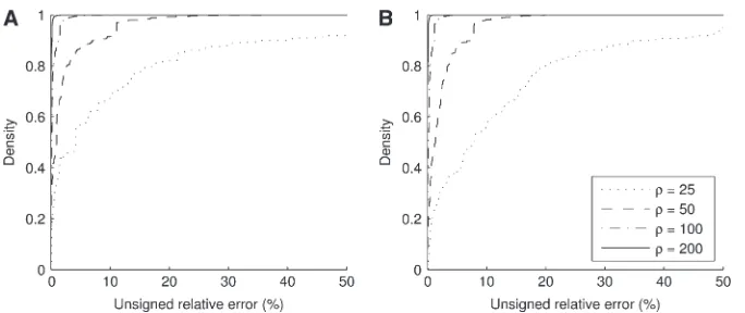
By comparing the performance ofqASFð0;0;cÞagainst that ofq0ð0;0;cÞandq0ð0;0;cÞ1q1ð0;0;cÞ=r, we can gain an idea of how much improvement is provided by each additional term in qASFð0;0;cÞ. As motivation, consider the likelihood curves shown in Figure 1, a and b, which compare different levels of approximation with the true likelihood for the configurationsð0;0;cÞwith c¼ 10 2
7 1
andc¼ 10 2 1 7
, respectively, foru¼0.01. The former is illustrative of a configuration for which the MLE ofr is infinite, and the latter is an example for which the MLE is finite. These configurations have sample sizes small enough that the true likelihoods can be solved directly from Equation 5. We can make a number of preliminary observations from Figure 1. As more terms are added to the ASF, it sustains a higher accuracy, as we would hope. In particular,qASFð0;0; cÞ seems to approximate the true likelihood very accu-rately forr $20. As illustrated in Figure 1, a similar level of accuracy is achieved by˜qASFð0;0;cÞ, an approxima-tion toqASFð0;0;cÞdefined by
˜qASFð0;0;cÞ ¼q0ð0;0;cÞ1q1ð0;0;cÞ
r 1
sð0;0;cÞ
r2 :
Recall thatq2ð0;0;cÞcomprises two terms (cf. Theorem 2): q2ðcA;cB;0Þ, which must be solved by dynamic
programming, andsð0;0; cÞ, for which we derived an analytic expression. Calculatingq2ðcA; cB;0Þimposes a
small computational burden compared to solving (5)
directly, but the associated running time grows with sample size. The approximation ˜qASFð0;0;cÞ simply ignores this potentially burdensome term. As we discuss later, in general this seems to lead to a negligible sacrifice in accuracy. Empirically, for most configura-tions we examined,q2ðcA;cB;0Þis at least an order of
magnitude smaller than the analytic termsð0;0;cÞ. We return to this below and carry out a more thorough study of the relative contribution of q2ðcA;cB;0Þ to
qASFð0;0;cÞ.
Distribution of unsigned relative errors: To ensure that the above results were not unique to the particular choices of data set illustrated, we performed a more systematic study as follows. For a givenc, we measure the accuracy ofqASFð0;0;cÞby theunsigned relative error
qASFð0
;0;cÞ qð0;0;cÞ qð0;0;cÞ
3100%;
with corresponding definitions for the unsigned relative errors of q0ð0;0;cÞ, q0ð0;0;cÞ1q1ð0;0; cÞ=r, and ˜qASFð0;0;cÞ. By drawing ð0;0;cÞaccording to the true sampling probability, we may speak of the distribution of the unsigned relative error. This distribution forms the basis of our measure of accuracy, and when calculating it, we must be sure to weight each sample correctly. The correct weight forð0;0;cÞisqð0;0;cÞtimes a combina-torial factor capturing the number of distinct orderings of the sample; this product is denoted bypð0;0;cÞ. To evaluateqð0;0;cÞ, we looked at sample sizes sufficiently small so that the true likelihood could be calculated directly by solving Equation 5. We implemented a com-puter program for solving the recursion numerically.
We can make one further efficiency saving. Comput-ing the true probabilityqð0;0;cÞfor every configuration of sizec$30 is computationally demanding. However, when mutation rates are the same for the two loci, observe that, by symmetry, distinct configurations exist with the same sampling probability. For example, the samplesc¼ x y
y x
andc¼ y x x y
are distinct observations when x, yare distinct nonnegative integers, but their sampling probabilities are the same. We can therefore collapse our space of distinct sample configurations into a smaller one of equivalence classes, where two distinct samples are considered equivalent if they have the same Figure 1.—Likelihood curves for r, comparing different levels of approxi-mation. A symmetric, finite-alleles model withu¼0.01 is assumed, as de-scribed in the text. The true likelihood is shown as a thick solid line. Formulas compared are q0ð0;0;cÞ (dotted line),
q0ð0;0;cÞ1q1ð0;0;cÞ=r (dashed line),
qASFð0;0;cÞ (thin solid line), and
˜qASFð0;0;cÞ(dotted-dashed line, largely concealed by the thin solid line). (a)
c¼ 10 7 2 1
. (b)c¼ 10 1 2 7
probability. Forc¼30, this meant that for 5456 distinct configurations only 752 probabilities required evalua-tion. Similar arguments can be made for the infinite-alleles model.
For the finite-alleles PIM models described above, the cumulative distribution of the unsigned relative error across all dimorphic samples of size c ¼ 20 is shown in Figure 2. As is clear from the plot, the ASF offers substantial accuracy even for r as ‘‘low’’ as 50. For example, for a dimorphic sample ð0;0;cÞ of size 20 drawn at random from pð0;0;cÞ with u ¼ 0.01, the probability that its ASFqASFð0;0;cÞis within 1% of the truth is 0.61, while the probability that qASFð0;0;cÞ is within 5% of the truth is 0.87. The corresponding probabilities when usingq0ð0;0;cÞalone are 0.36 and 0.43, respectively. Note the spike of probability mass around zero even for the curve for q0ð0;0;cÞ. This suggests that assuming r ¼ ‘ will still be accurate in about half of cases, but with substantial errors in the rest. This is not the case when employingqASFð0;0;cÞinstead. The distributions for the two mutation parameters are rather similar, suggesting a certain degree of robustness in the ASF tou. The case withu ¼1 seems to have a lower probability of achieving a high accuracy (say within 1%) but a higher probability of achieving a moderate accuracy (within 10%).
Effect of sample size and recombination rate: To assess the sensitivity ofqASFð0;0;cÞto the sample sizec and the recombination rate r, we repeated the above plots for varying values of these parameters; results are shown in Figures 3 and 4. As we might expect, accuracy
improves with increasing r. For example, for u¼0.01 andr¼200, the probability of drawing a sampleð0;0;cÞ with qASFð0;0;cÞwithin 1% of the truth reaches 1.00, compared with a probability of 0.54 when using q0ð0;0;cÞalone. On the other hand, for a fixedr, the accuracy of qASFð0;0;cÞ generally begins to diminish with increasing c. One possible explanation for this trend is that larger samples may have more subtle shapes to their likelihood curves, such as multiple turning points. The ASF effectively has to fit a curve with at most one turning point to approximate qð0;0;cÞ with high accuracy for large r. This might be at the expense of accuracy for smallerr(see also Figure 9 later).
Signed relative error: Using the unsigned relative error as a measure of accuracy loses information on the question of whether the ASF systematically under- or overestimates the true sample probability. To investigate this, we calculated the expected signed relative error ðqASFð0;0;cÞ qð0;0;cÞÞ=qð0;0;cÞ3100% across all configurations for each combination of parameters con-sidered above. The signed relative errors of q0ð0;0;cÞ;
q0ð0;0;cÞ1q1ð0;0;cÞ=r, and ˜qASFð0;0;cÞ are defined similarly. The results are given in Tables 1 and 2. Although most of these expectations are positive, they are generally very small, and all fall within61.25%. This suggests that if deviations from the true likelihood tend to err in a particular direction, then this skewness is negligible.
Monomorphic samples:One might argue that exclud-ing nonsegregatexclud-ing sites from the analyses above is unwarranted, since the observation that a site is non-segregating also contains information about the parameters Figure 2.—Cumulative distribution of unsigned relative error of q0ð0;0;cÞ (dotted line), q0ð0;0;cÞ1q1ð0;0;cÞ=r (dashed line),˜qASFð0;0;cÞ(dotted-dashed line, almost concealed by the solid line), andqASFð0;0;cÞ (solid line). We consid-ered dimorphic sample configurations ð0;0;cÞ drawn from pð0;0;cÞ in the finite-alleles model withc¼20 andr¼ 50. (a)u¼0.01. (b)u¼1.
Figure 3.—The effect of varying c (fixing r¼ 50). Plotted is the cumula-tive distribution of the unsigned relacumula-tive error ofqASFð0;0;cÞacross all dimorphic sample configurations of size c ¼ 10 (solid line), c¼20 (dashed line), and
of the model. We therefore reanalyzed the distribution of the unsigned relative error across all samples of sizec¼ 20 (withr ¼50), rather than just dimorphic samples. Results are shown in Figure 5.
Compare Figure 5 with Figure 2 (note the different scales on thex-axes). Clearly, across all samples there is now a much greater level of accuracy, particularly when the mutation rate is small. This may be explained by the following two observations. First, the probability that one or both loci are monomorphic is relatively large: foru¼0.01 it is.0.99 and foru¼1.0 it is 0.44. Hence, these configurations will have a substantial effect on the error distribution, particularly for smaller mutation rates. Second, the ASF seems to be much more accurate precisely for those configurations with one or both loci monomorphic. This raises the question: Can we identify any further patterns for which the ASF is more accurate? When the true likelihood is unavailable, this might provide a guide as to how accurate the ASF is likely to be. For which samples is the ASF most accurate? The figures described above suggest that for most config-urations the relative error of the ASF will be very small, with a few having larger errors. It would be of interest to determine whether there is any feature of a given sample configuration that indicates how accurate the ASF will be. Figure 6 plots on a log-scale the unsigned relative error of the ASF of a sample against its sampling probabilitypð0;0;cÞ, across all configurations of sample size c ¼ 20 (with u ¼ 0.01 and u ¼ 1, and r ¼ 50).
Encouragingly, there is a clear negative correlation between unsigned relative error and sampling proba-bility (Pearson’s correlation coefficient ¼ 0.76 for Figure 6a and 0.61 for Figure 6b). That is, those configurations for which the ASF is most accurate are also observed most often. However, the point of this comparison is to determine which configurations have a more accurate ASFwithouthaving to calculatepð0;0;cÞ. We therefore identified the following categories for the samples that appear to best explain most of the variation in accuracy (the category of each sample is annotated in Figure 6):
1. ,, the sample is monomorphic at both loci. 2. n, the sample is monomorphic at one locus. 3. s, for at least one allele at a locus, the sample has
multiplicity one; i.e., a row or column ofcsums to one.
4. 1, the sample has very low linkage disequilibrium (LD) as measured by r2(Hudson2001b), satisfying r2# 0.02. (This LD measure is also often denoted byD2.)
5. e, the sample is in perfect LD;i.e., it is of the form c¼ x 0
0 y
or 0x 0y
, wherex1y¼c, forx$0 andy$0. 6. h, the sample is in perfect LD except for one
haplotype; i.e., it is of the form c¼ x 1 0 y
, x1 0y
, 1 y
x 0
, or 0x y1
, wherex1 y¼c1, forx$0 and y$0.
7. d, the sample does not fall into any of the above categories.
Some configurations fell into more than one category, in which case the higher category in this list was given priority.
Figure 6a confirms that samples monomorphic at one or both loci have among the highest sampling proba-bilities and the highest accuracies. This is followed by another clearly identifiable cluster of samples of high accuracy, which have in common that one allele has multiplicity one. For the remaining samples, the amount of LD seems to be highly informative of the accuracy of the ASF; for example, at the upper end of the error distribution are those in perfect or almost perfect LD. We do not have an intuitive explanation for Figure 4.—The effect of varying r (fixingc¼20). Plotted is the cumula-tive distribution of the unsigned relacumula-tive error of qASFð0;0;cÞ across all dimor-phic sample configurations of sizec¼ 20 for r ¼ 200 (solid line), r ¼ 100 (dotted-dashed line), r ¼ 50 (dashed line), andr¼25 (dotted line). (a)u¼ 0.01. (b)u¼1.
TABLE 1
Expected signed relative error (percentage) for different approximations across all dimorphic samples withc¼20
r
25 50
u¼0.01 u¼1.0 u¼0.01 u¼1.0
q0ð0;0;cÞ 0.48 0.12 0.21 0.06
q0ð0;0;cÞ1q1ð0;0;cÞ=r 0.32 0.06 0.12 0.03
˜qASFð0;0;cÞ 0.10 0.01 0.07 0.01
this observation. Most of the remaining samples fall around a cluster of intermediate accuracy (1%), with the samples with lowest LD at the center of this cluster. For higher mutation rates, illustrated in Figure 6b, we observed a similar, albeit less distinguished, pattern. When mutation rates are higher, the difference in pro-bability between any two sample configurations tends to be attenuated. We also observed qualitatively similar patterns for different choices of sample size and recom-bination rate (not shown).
A quick approximation to the ASF: Recall that q2ða;b;cÞcontains a term—namely,q2ða1cA;b1cB;0Þ—
that needs to be evaluated recursively using dynamic programming. (See Theorem 2.) This imposes a small but growing (with sample size) computational burden on the calculation ofqASFða;b;cÞ. Empirical tests (for exam-ple, Figure 2) suggested that simply ignoringq2ða1cA;
b1cB;0Þleads to almost no loss in accuracy. It is worth
addressing the contribution of this term in more detail. We measure its contribution by the following quantity:
qASFða;b;cÞ ˜qASFða;b;cÞ
qASFða;b;cÞ 3100%
¼ 1
r2
q2ða1cA;b1cB;0Þ
qASFða;b;cÞ 3100%: ð11Þ
As before, we weight this contribution by the sampling probabilitypða;b;cÞof each configuration. Its distribu-tion is shown in Figure 7, for dimorphic samples of size c¼20 andr¼50.
It is clear from Figure 7 that for these parameter values, using ˜qASFð0;0;cÞin place ofqASFð0;0;cÞaffects the result by no more than 1%, and with a high probability the effect is ,0.2%. Indeed, when u ¼1, the contribution is,0.2% with an estimated probability of 1. These results are encouraging. They suggest that we may safely discard theq2ða1cA;b1cB;0Þterm
with-out a considerable loss of accuracy. This also seems to hold for larger sample sizes. For all samples of size c ¼100, one can still calculate the contribution (11), although it is now computationally impractical to weight each sample by its true probabilitypð0;0;cÞ. Instead we looked at thenumberof sample configurations within a given range of contributions. For example, whenr¼50 andu¼0.01, the contribution (11) was within the range6
0.5% for 93.2% of dimorphic samples of size c ¼ 100. Whenu¼1, 95.7% of dimorphic sample configurations were within this range. Thus, even for larger sample sizes, when calculating the term q2ða1cA;b1cB;0Þbecomes
impractical, using the approximation ˜qASFð0;0;cÞseems to be an attractive option. For the infinite-alleles model, we ( Jenkins and Song 2009) have obtained a close upper
bound to estimate the contribution of this term whenever calculating it directly is computationally intractable.
DISCUSSION
Computing likelihoods under the coalescent with recombination is a challenging problem that has re-ceived much attention in the past. Here, building on our recent work ( Jenkinsand Song2009), we provided TABLE 2
Expected signed relative error (percentage) ofqASF(0, 0, c) across all dimorphic samples
r
25 50 100 200
c u¼0.01 u¼1.0 u¼0.01 u¼1.0 u¼0.01 u¼1.0 u¼0.01 u¼1.0
10 0.60 0.27 0.11 0.05 0.02 0.01 0.00 0.00
20 0.93 0.28 0.19 0.06 0.03 0.01 0.01 0.00
30 1.21 0.28 0.26 0.06 0.05 0.01 0.01 0.00
Figure5.—A repeat of Figure 2 but across all samples rather than all dimor-phic samples (c¼20,r¼50). Note the different scales on thex-axes. The curves show the distribution of the unsigned relative error ofq0ð0;0;cÞ(dotted line),
q0ð0;0;cÞ1q1ð0;0;cÞ=r (dashed line),
˜qASFð0;0;cÞ (dotted-dashed line, con-cealed by the solid line), and
an alternative perspective on the likelihood computa-tion and obtained analytic results for the two-locus model with an arbitrary finite-alleles model of mutation. As mentioned in the Introduction, a stochastic process may exist that is simpler than the well-established co-alescent with recombination that captures the impor-tant dynamics of the relevant degrees of freedom as the rate of recombination gets large. We think that the fact that the first-order termq1ða;b;cÞ[see (8)] is so simple supports this speculation. Foru¼1, the Ewens sampling formula for the one-locus infinite-alleles model reduces to the classic formula for the joint distribution of cycle counts in a random permutation (see Arratia et al.
2003 for a discussion of this and other combinatorial connections). It would be interesting to provide such a combinatorial interpretation of q1ða;b;cÞ. Further, we believe that finding a closed-form expression for the first-order term for more than two loci might be possible.
As a concrete application of our asymptotic sampling formula, one can analytically compute, for large values ofr, the expectation of linkage disequilibrium measures such asr2. Songand Song(2007) showed analytically that the populationwide expectation of r2approaches 1/rasr/‘. For a finite sample sizen, Hilland Weir
(1994) derivedð1=ð11rÞÞð11=nÞ11=nfor the sam-plewise expectationE[r2] ofr2. This result was obtained under restrictive assumptions that the populationwide marginal allele frequencies are all1
2 and that
heterozy-gote superiority holds at each locus. For a given sample size n, it would be interesting to use our asymptotic sampling formula to derive a general asymptotic expres-sion for the samplewise expectationE[r2].
Below we discuss in detail two other concrete appli-cations of our sampling formula. First, we discuss how we can improve the composite-likelihood method (Hudson 2001a). Then, we provide the first analytic
result on the classification of the MLE ofr.
Composite-likelihood method:LDhat (McVeanet al.
2002, 2004) is a software package aimed at using pat-terns of variation in population genetic data to estimate fine-scale recombination rates. The procedure is effi-cient and has been applied to genomewide estimates of the human genetic map (Myerset al.2005; I nterna-tional Hapmap Consortium 2007) (henceforth, we
assume that recombination events are always resolved as crossovers and ignore the effects of homologous gene conversion). Part of its efficiency stems from the use of the pairwise composite likelihood first proposed by Hudson(2001a). For a given genetic map, LDhat
em-ploys a Bayesian reversible-jump Markov chain Monte Carlo (rjMCMC) procedure to propose updates to this map and to sample from an approximate posterior distribution (the approximation resulting from the use of a pseudolikelihood defined below). To calculate the acceptance probabilities of proposed moves, one must calculate the likelihood of the data. To do so exactly (e.g., by solving a multilocus version of Equation 5) or Figure6.—The relationship between unsigned relative error of the ASF and a configuration’s sample probability
pð0;0;cÞ, across all configurations of sizec¼20 withr¼50. Configurations are categorized as monomorphic at both loci (=), monomorphic at one lo-cus (n), one or both loci have a
single-ton allele (s), very low LD (1), in perfect LD (e), in perfect LD except
for one haplotype (h), and the rest
(d). See text for details of these
defini-tions. (a)u¼0.01. (b)u¼1.0.
Figure7.—Distribution of the contri-bution (11) ofq2ðcA;cB;0ÞtoqASFð0;0;cÞ, with respect to dimorphic samples of size
even by a computationally intensive full-likelihood pro-cedure such as importance sampling (Fearnheadand
Donnelly 2001) is highly impractical for the sizes of
data sets of interest. To circumvent this problem, Hudson
(2001a) proposed the composite-likelihood method and showed that it works very well as an estimator forr. This method uses two-locus likelihoods as building blocks and LDhat uses the following variation on the theme: Suppose that the input data setDcontainsmpolymorphic sites, and letDijdenote the data set restricted to the two sitesiandj.
Then, the composite likelihood is defined as
LCðrÞ ¼Y i,j
pðDijÞ: ð12Þ
In this formula,ris assumed to be constant across the region and the probability associated with each pair uses a rescaled value forrto account for the physical distance between the pair. It is straightforward to modify this definition to allow for variable recombination rates, as implemented in LDhat. The composite-likelihood ap-proximation treats the collection {Dij:i ,j andi,j¼
1,. . .,m} as m2 independent observations. Of course, in reality these observations are highly dependent through their shared ancestry, but often in practice little in-formation about the MLE ofr is lost. The key to this approach is that it is much more straightforward to calculate each term in the product (12) than it is to cal-culate the full likelihood, since now one has to deal only with two sites at any one time. Hudson (2001a)
considered an infinite-sites model in the limit asu/0, conditional on the observed variation. McVean et al.
(2002) extended this approach to finite-alleles models and finiteuand used the importance sampling scheme of Fearnheadand Donnelly(2001) to estimate each
of these two-site likelihoods. This importance sampling stage is the most computationally intensive part of the LDhat estimation procedure. By considering all possible pairwise sample configurations of a given size, it is possible to precompute these likelihoods, and indeed the LDhat software package is accompanied by precom-puted lookup tables for various sample sizes and muta-tion rates. For each sample configuramuta-tion and mutamuta-tion rate, the likelihood is calculated over a grid ofr-values known as thedriving values; the default choice is over the integers r ¼0, 1,. . ., 100. Genetic distances are then rounded to the nearest integer. For pairs of sites whose genetic distance is.100, the two-site likelihood simply truncatesrto 100 and uses this precomputed value for the likelihood instead.
Here, we investigate the effect that this truncation has on the two-site likelihood. Since the ASF applies to the diallelic, symmetric mutation model employed by LDhat, an obvious alternative to truncation is to use the ASF. As r increases, we expect the truncation procedure to introduce more error, while the ASF becomes more accurate. Furthermore, the ASF is a continuous function ofrand so no further error is introduced by rounding to
the nearest driving value ofr. Assuming a recombination rate of 1 cM/Mb (Konget al.2002) and a human diploid
effective population size of 10,000 (Myerset al.2005), a
cutoff ofr¼100 corresponds to a marker separation of 250 kb. In the presence of recombination hotspots this distance could be much lower. The study of Myerset al.
(2005) breaks up genomewide data into windows of 2000 SNPs, using a data set with an average marker spacing of 1.9 kb (Hindset al.2005). A rough approximation to the
mean window size is thus3.8 Mb; pairs of sites separated by a distance .r ¼100 are therefore encountered fre-quently by the rjMCMC procedure.
Using its estimate of the likelihood atr¼100, LDhat encounters two sources of error: one from the trunca-tion of the range ofrand one from the stochastic error of the importance sampling procedure. To restrict our attention to the first of these sources, we find a lower bound on the error of LDhat by looking at the quantity
Lð
rÞ Lð100Þ LðrÞ
3100%;
whereL(r) is thetruelikelihood obtained previously by solving Equation 5. The true likelihood atr¼100 will of course be at least as accurate an approximation as that reported by LDhat. Table 3 reports the mean unsigned relative error one would obtain usingL(100) in place of L(r), for various choices of r and various choices of mutation rates used by the lookup tables in LDhat. For comparison we also show the unsigned relative error of LASFðrÞ:¼qASFð0;0;cÞ. In Figure 8, we also show the complete distribution of these errors for one set of parameters in the table, namely,c¼30 andu¼0.002. (Note that this choice of mutation rate would be re-ported asu¼0.001 in LDhat, since it uses the mutation transition matrix P¼ 0 1
1 0
at each locus instead of P¼ 1=2 1=2
1=2 1=2
used here.) Sinceris not fixed throughout the rjMCMC procedure, it is not clear in this setting how to interpret the idea of drawing a sample configuration
TABLE 3
The mean unsigned relative error (percentage) ofL(100) and ofLASF(r) compared to the true likelihoodL(r), across all
dimorphic samples of sizec
c¼20: c¼30:
r r
u 100 150 200 250 100 150 200 250
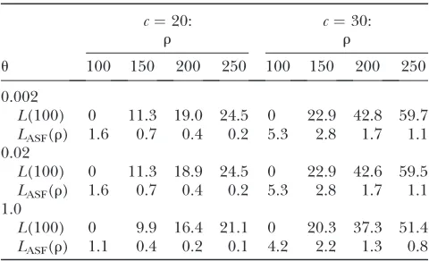
0.002
L(100) 0 11.3 19.0 24.5 0 22.9 42.8 59.7
LASF(r) 1.6 0.7 0.4 0.2 5.3 2.8 1.7 1.1
0.02
L(100) 0 11.3 18.9 24.5 0 22.9 42.6 59.5
LASF(r) 1.6 0.7 0.4 0.2 5.3 2.8 1.7 1.1
1.0
L(100) 0 9.9 16.4 21.1 0 20.3 37.3 51.4
at random. Here, we therefore take a simple arithmetic mean unsigned relative error across all dimorphic sam-ples, rather than weighting each configuration by its sampling probabilitypð0;0;cÞas before.
As is clear from Table 2, using L(100) as a proxy forL(r) whenr.100 rapidly becomes very inaccurate with increasingr. Even for these moderate sample sizes, there may be a considerable amount of information in the sample so that the likelihoods atr¼100 andr ¼ 200, say, differ substantially. For the sample sizes con-sidered here, using the ASF instead of LDhat becomes preferable very soon abover¼100 and certainly before r¼150. For larger samples the critical point at which the ASF becomes preferable may be somewhat higher. Also, note that the error in both methods seems to be highly robust to the choice of mutation rate, at least for the set of realistic choices shown. For both methods, there is a slight decrease in error rate with increasing mutation rate.
Figure 8 confirms the wider distribution of errors when usingL(100) to estimateL(200) rather than using LASF(200). Since we plot here the signed relative error rather than the unsigned relative error, we are also able to observe that the distribution of errors is not symmet-ric about zero; there is much more probability mass on nonnegligible positive relative errors than on negative relative errors. This suggests that LDhat could system-atically overestimate the likelihood of pairs of markers for which a large recombination rate is proposed, bias-ing recombination rate estimates upward; proposed alterations to the genetic map that increase the recom-bination rate in a region will have erroneously inflated acceptance rates. When usingLASF(r), the asymmetry in errors is much smaller.
Classification of the MLE ofr:The ASF can be used to make inferences about whether or not the MLE ofr is finite. Intuitively, when q1ða;b;cÞ.0, the asympto-tic approximation q0ða;b;cÞ1q1ða;b;cÞ=r approaches q0ða;b;cÞfrom above asr/‘. Moreover, by virtue of it being an asymptotic approximation, for large enoughr it must be sufficiently accurate to infer that qða;b;cÞ must also approachq0ða;b;cÞfrom above. We therefore have the following theorem, for which a formal proof
may be given via a short analysis argument (in the
appendix):
Theorem3.For a given sample configurationða;b;cÞ, if
the first-order termq1ða;b;cÞ[see (8)]in the asymptotic expansion satisfies
q1ða;b;cÞ.0;
then the MLE ofris finite.
If one-locus marginal sampling probabilities are known, as in the infinite-alleles case or the PIM case, then q1ða;b;cÞis instantaneous to compute. To our knowledge, Figure8.—Distribution of signed rel-ative errors (%) of (a)L(100) and (b)
LASF(200) when estimating L(200), across all dimorphic configurations of sizec ¼ 30. The mutation rate is u¼ 0.002.
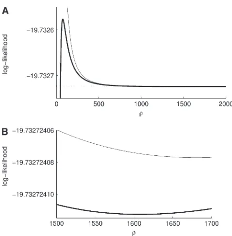
Figure9.—(a) Example with a local minimum and a local maximum in the likelihood curve forr. This example is for
c¼ 6 3 1 0
this is the first analytic result on the classification of the MLE ofr. Note, however, that this is a sufficient condition, but not a necessary condition. That is, this condition does not identifyall samples with a finite MLE. Indeed, it is tempting to argue for the converse to the proposition above—namely, that q1ða;b;cÞ,0 implies an infinite MLE—but this is false, as the following simple counter-example demonstrates.
Consider the sample configuration ð0;0;cÞ deter-mined byc¼ 6 1
3 0
, and supposeu¼0.01. It is straight-forward to verify thatq1ð0;0;cÞ,0 but thatr0exists with L(r0). L(‘). The likelihood curve for this configura-tion can be found by solving Equaconfigura-tion 5 directly and is illustrated in Figure 9. Although the curve approaches the asymptoteL(‘)ð¼q0ð0;0;cÞÞfrom below asr/‘
[as one expects whenq1ða;b;cÞ,0], it actually exhibits a local minimum atr¼1608, as well as a local maximum farther down atr¼74. In this example the likelihood curve is extremely flat, but minima with higher curva-ture may be found for larger sample sizes. To our knowledge, this is the first confirmation of a local minimum in a likelihood curve forr.
We thank Fulton Wang for writing a computer program that numerically solves two-locus recursions and Rasmus Nielsen and Monty Slatkin for helpful comments. This research is supported in part by a National Institutes of Health grant R00-GM080099 (to Y.S.S.), an Alfred P. Sloan Research Fellowship (to Y.S.S.), and a Packard Fellowship for Science and Engineering (to Y.S.S.).
LITERATURE CITED
Arratia, A., A. D. Barbourand S. Tavare´, 2003 Logarithmic
Com-binatorial Structures: A Probabilistic Approach.European Mathemat-ical Society Publishing House, Zurich, Switzerland.
DeIorio, M., and R. C. Griffiths, 2004a Importance sampling on coalescent histories I. Adv. Appl. Probab.36:417–433. DeIorio, M., and R. C. Griffiths, 2004b Importance sampling on
coalescent histories II. Adv. Appl. Probab.36:434–454. Ethier, S. N., and R. C. Griffiths, 1990 On the two-locus sampling
distribution. J. Math. Biol.29:131–159.
Ewens, W. J., 1972 The sampling theory of selectively neutral alleles. Theor. Popul. Biol.3:87–112.
Fearnhead, P., and P. Donnelly, 2001 Estimating recombination rates from population genetic data. Genetics159:1299–1318. Golding, G. B., 1984 The sampling distribution of linkage
disequi-librium. Genetics108:257–274.
Griffiths, R. C., 1981 Neutral two-locus multiple allele models with recombination. Theor. Popul. Biol.19:169–186.
Griffiths, R. C., and P. Marjoram, 1996 Ancestral inference from samples of DNA sequences with recombination. J. Comput. Biol. 3:479–502.
Griffiths, R. C., and S. Tavare´, 1994 Simulating probability distri-butions in the coalescent. Theor. Popul. Biol.46:131–159. Griffiths, R. C., P. A. Jenkinsand Y. S. Song, 2008 Importance
sampling and the two-locus model with subdivided population structure. Adv. Appl. Probab.40:473–500.
Hill, W. G., and B. S. Weir, 1994 Maximum-likelihood estimation of gene location by linkage disequilibrium. Am. J. Hum. Genet. 54:705–714.
Hinds, D. A., L. L. Stuve, G. B. Nilsen, E. Halprein, E. Eskinet al.,
2005 Whole-genome patterns of common DNA variation in
three human populations. Science307:1072–1079.
Hudson, R. R., 1983 Properties of a neutral allele model with intra-genic recombination. Theor. Popul. Biol.23:183–201. Hudson, R. R., 2001a Two-locus sampling distributions and their
application. Genetics159:1805–1817.
Hudson, R. R., 2001b Linkage disequilibrium and recombination, Chap. 11 inHandbook of Statistical Genetics, edited by D. Balding, M. Bishopand C. Cannings. Wiley, Chichester, UK.
InternationalHapMapConsortium, 2007 A second generation
human haplotype map of over 3.1 million SNPs. Nature 449:
851–861.
Jenkins, P. A., and Y. S. Song, 2009 An asymptotic sampling formula for the coalescent with recombination. Ann. Appl. Probab. (in press). Available as Technical Report 775. Department of Statistics, University of California, Berkeley, CA (http://www.stat. berkeley.edu/tech-reports).
Kingman, J. F. C., 1982a On the genealogy of large populations. J. Appl. Probab.19:27–43.
Kingman, J. F. C., 1982b The coalescent. Stoch. Proc. Appl.13:235– 248.
Kong, A., D. F. Gudbjartsson, J. Sainz, G. M. Jonsdottir, S. A. Gudjonsson et al., 2002 A high-resolution recombination
map of the human genome. Nat. Genet.31:241–247.
Kuhner, M. K., J. Yamatoand J. Felsenstein, 2000 Maximum like-lihood estimation of recombination rates from population data.
Genetics156:1393–1401.
Lundstrom, R., S. Tavare´and R. H. Ward, 1992 Modeling the
evo-lution of the human mitochondrial genome. Math. Biosci.112:
319–335.
Lyngsø, R. B., Y. S. Songand J. Hein, 2008 Accurate computation of likelihoods in the coalescent with recombination via parsi-mony, pp. 463–477 inProceedings of the 12th Annual International Conference on Research in Computational Molecular Biology (RECOMB)(Lecture Notes in Computer Science, Vol. 4955), edi-ted by M. Vingronand L. Wong, Springer, Berlin/Heidelberg, Germany.
McVean, G., P. Awadallaand P. Fearnhead, 2002 A coalescent-based method for detecting and estimating recombination from
gene sequences. Genetics160:1231–1241.
McVean, G. A. T., S. R. Myers, S. Hunt, P. Deloukas, D. R. Bentley
et al., 2004 The fine-scale structure of recombination rate
vari-ation in the human genome. Science304:581–584.
Myers, S., L. Bottolo, C. Freeman, G. McVeanand P. Donnelly,
2005 A fine-scale map of recombination rates and hotspots
across the human genome. Science310:321–324.
Nachman, M. W., and S. L. Crowell, 2000 Estimate of the muta-tion rate per nucleotide in humans. Genetics156:297–304. Nielsen, R., 2000 Estimation of population parameters and
recom-bination rates from single nucleotide polymorphisms. Genetics 154:931–942.
Song, Y. S., and J. S. Song, 2007 Analytic computation of the expec-tation of the linkage disequilibrium coefficientr2. Theor. Popul.
Biol.71:49–60.
Stephens, M., and P. Donnelly, 2000 Inference in molecular pop-ulation genetics. J. R. Stat. Soc. B62:605–655.
Wang, Y., and B. Rannala, 2008 Bayesian inference of fine-scale re-combination rates using population genomic data. Philos. Trans. R. Soc. B363:3921–3930.
Wright, S., 1949 Adaptation and selection, pp. 365–389 in
Ge-netics, Paleontology and Evolution, edited by G. L. Jepson, E. Mayrand G. G. Simpson. Princeton University Press, Prince-ton, NJ.
APPENDIX
The proofs given here are similar in structure to our previous proofs ( Jenkinsand Song2009) for the
infinite-alleles model of mutation. It turns out that much of the argument is independent of the particular model of mutation assumed. Therefore, we give only an outline here and refer the reader to that article for further details.
Proof of Proposition1. The infinite-alleles case was proved in Jenkinsand Song(2009), so we focus on the finite-alleles
case here. First, assumec . 0. One can obtain a recursion satisfied by q0ða;b;cÞ by substituting our asymptotic expansion (6) into (5), dividing byrc, and lettingr/‘. We obtain
q0ða;b;cÞ ¼X K
i¼1
XL
j¼1 cij
c q0ða1ei;b1ej;ceijÞ: ðA1Þ
By repeated application of (A1) this becomes
q0ða;b;cÞ ¼q0ða1cA;b1cB;0Þ; ðA2Þ which of course also holds whenc¼0. Now, by substituting (6) into (5) withc¼0and then lettingr/‘, we obtain [after some manipulation, invoking (A2) to eliminate terms for whichc.0]
½aða1uA1Þ1bðb1uB1Þq0ða;b;0Þ
¼X K i¼1
aiðai1Þq0ðaei;b;0Þ1
XL
j¼1
bjðbj1Þq0ða;bej;0Þ
1uA
XK
i¼1 ai
XK
k¼1
PkiAq0ðaei1ek;b;0Þ1uB
XL
j¼1 bj
XL
l¼1
PljBq0ða;bej;0Þ: ðA3Þ
Boundary conditions areq0ðei;0;0Þ ¼1 fori¼1,. . .,Kandq0ð0;ej;0Þ ¼1 forj¼1,. . .,L. It is straightforward to verify
that the solution to (A3) is
q0ða;b;0Þ ¼qAðaÞqBðbÞ; ðA4Þ whereqAðaÞandqBðbÞare marginal one-locus sampling probabilities for lociAandB, respectively. Together, (A2) and
(A4) give the desired result. n
Proof of Theorem1. Again, the infinite-alleles case was proved in Jenkinsand Song(2009), so we focus on the
finite-alleles case here. Substitute the asymptotic expansion (6) into the recursion (5), eliminate terms of orderrby applying (A1), and letr/‘. After invoking (A3) and (7), with some rearrangement we obtain
q1ða;b;cÞ ¼fða;b;cÞ1X
K
i¼1
XL
j¼1 cij
c q1ða1ei;b1ej;ceijÞ; ðA5Þ
where
fða;b;cÞ:¼ ðc1ÞqAða1cAÞqBðb1cBÞ
qBðb1cBÞX K i¼1
ciðci1Þ
c q
Aða1cAeiÞ
qAða1cAÞ
XL
j¼1
cjðcj1Þ
c q
Bðb1c BejÞ
1 X
K i¼1
XL
j¼1
cijðcij1Þ
c q
Aða1c
AeiÞqBðb1cBejÞ: ðA6Þ
Above we assumedc.0; we definefða;b;cÞ ¼0 ifc¼0.
q1ða;b;cÞ ¼X c m¼1
E½fðAðmÞ;
BðmÞ;CðmÞÞ; ðA7Þ
where CðmÞ
is the random subsample obtained by selecting m gametes from the sample c uniformly without replacement; that is, it is distributed according to a multivariate hypergeometric distribution with parametersðc;c;mÞ. Further, we defineAðmÞ¼
a1cACðmÞandBðmÞ¼b1cBCðmÞ. The expectations in (A7) are easy to compute and to
sum overm, resulting in (8). n
Proof of Theorem2. In a similar manner to the proof of Theorem 1, one can show that
q2ða;b;cÞ ¼q2ða1cA;b1cB;0Þ1 X
c m¼1
E½gðAðmÞ;
BðmÞ;CðmÞÞ; ðA8Þ
where gða;b;cÞ has a known, but rather cumbersome, closed-form expression. Since these expectations can be evaluated, the sumPcm¼1E½gðAðmÞ;
BðmÞ;CðmÞÞ
composes the closed-form part ofq2ða;b;cÞ;i.e.,
sða;b;cÞ ¼X c
m¼1
E½gðAðmÞ;BðmÞ;CðmÞÞ:
Unlike the form offða;b;cÞ, that ofgða;b;cÞdepends on the model of mutation. We repeated the steps in Jenkinsand
Song(2009) using Equation 5—rather than Golding’s recursion (Golding1984), which applies to the infinite-alleles
model—to obtain the following expression forsða;b;cÞ. We omit the simple but lengthy algebraic details. LetQAdenoteqAða1c
AÞ,QiAdenoteqAða1cAeiÞ,QikA denoteqAða1cAeiekÞ, and so on. Then,
sða;b;cÞ ¼c 3
ðc1Þðc11Þð3c2Þ
8 1ðc1Þð3a13b12c1Þ16ab
QAQB
1X
K
i¼1
uAcðc3Þ12a14b4
4 ciðci1Þ ð2b1c1Þciðai1ci1Þ
QAiQB
1X
L j¼1
uBcðc3Þ12b14a4
4 cjðcj1Þ ð2a1c1Þcjðbj1cj1Þ
QAQBj
1 1
12
XK
i¼1
ð56ai4ciÞciðci1ÞQAiiQB1 1 12
XL
j¼1
ð56bj4cjÞcjðcj1ÞQAQBjj
1X
K i¼1
XK
k¼1
ciðci1Þckðck1Þ
8 Q
A ikQB1
XL
j¼1
XL
l¼1
cjðcj1Þclðcl1Þ
8 Q
AQB jl
uA1uBcðc5Þ12a12b4 4
XK
i¼1
XL
j¼1
cijðcij1ÞQAiQBj
1X
K
i¼1
XL
j¼1
ciðci1Þcjðcj1Þ
4 1
cijðcij112ci12cicj2cjÞ 2
1cijbjðci1Þ1cijaiðcj1Þ12aibjcij
QAiQBj
11
2
XK
i¼1
ðai1ci1Þ XL
j¼1
cijðcij1ÞQAiiQ B j 1
1 2
XL
j¼1
ðbj1cj1Þ
XK
i¼1
cijðcij1ÞQAiQ B jj
1 4
XK
i¼1
XL
j¼1
XK
k¼1
cijðcij1Þckðck1ÞQAikQBj 1 4
XK
i¼1
XL
j¼1
XL
l¼1
cijðcij1Þclðcl1ÞQAiQBjl
11
8
XK
i¼1
XL
j¼1
XK
k¼1
XL
l¼1
cijðcij1Þcklðckl 1ÞQAikQBjl
1 12
XK
i¼1
XL
j¼1
cijðcij1Þð2cij1ÞQAiiQBjj
1lða;b;cÞ:
The final term, lða;b;cÞ, is a function whose form depends on the model of mutation. Using QiA,1t to denote
qAða1c
lða;b;cÞ ¼ uA 2
XK
i¼1
XK
k¼1
XK
t¼1
PtiAðdtkdikÞciðckdikÞQikA;1tQB
uB 2
XL
j¼1
XL
l¼1
XL
t¼1
PtjBðdtldjlÞcjðcldjlÞQAQjlB;1t
uA 4
XK
i¼1
XK
t¼1
PtiAciðci1ÞQiiA;1tQB uB
4
XL
j¼1
XL
t¼1
PtjBcjðcj1ÞQAQjjB;1t
1uA
2
XK
i¼1
XL
j¼1
XK
k¼1
XK
t¼1
PtiAðdtkdikÞcijðckjdikÞQikA;1tQjB
1uB
2
XK
i¼1
XL
j¼1
XL
l¼1
XL
t¼1
PtjBðdtldjlÞcijðcildjlÞQiAQjlB;1t
1uA
4
XK
i¼1
XL
j¼1
XK
t¼1 PA
ticijðcij1ÞQiiA;1tQjB1 uB
4
XK
i¼1
XL
j¼1
XL
t¼1 PB
tjcijðcij1ÞQiAQjjB;1t;
wheredijdenotes the Kronecker delta, and in a PIM model this simplifies to
lða;b;cÞ ¼ uAðc1Þ 2
XK
i¼1
ciPiAQiAQB
uBðc1Þ 2
XL
j¼1
cjPjBQAQjB
1uA
4
XK
i¼1
PiAciðci1ÞQiiAQB1 uB
4
XL
j¼1
PjBcjðcj1ÞQAQjjB
1X
K
i¼1
XL
j¼1
uB 2 P
B
j cijðci1Þ1 uA
2 P A
i cijðcj1Þ
QiAQjB
uA 4
XK
i¼1 PiAX
L
j¼1
cijðcij1ÞQiiAQ B j
uB 4
XL
j¼1 PjBX
K
i¼1
cijðcij1ÞQiAQ B jj:
For completeness, we also give the corresponding expression for the infinite-alleles model,
lða;b;cÞ ¼ uAðc1Þ 2
XK
i¼1
dai;0dci;1Q
A i QB
uBðc1Þ 2
XL
j¼1
dbj;0dcj;1Q AQB
j
1uA
2
XK
i¼1
dci;2Q
A iiQB1
uB 2
XL
j¼1
dcj;2Q AQB
jj
1X
K i¼1
XL
j¼1
uB
2 dbj;0dcj;1dcij;1ðci1Þ1 uA
2 dai;0dci;1dcij;1ðcj1Þ
QAiQBj
uA 2
XK
i¼1
XL
j¼1
dci;2dcij;2Q
A iiQjB
uB 2
XK
i¼1
XL
j¼1
dcj;2dcij;2Q A iQBjj
( Jenkinsand Song2009).
We now outline the steps to obtain the recursion shown in (10). One can use Equation A8 to show that
q2ðaei;bej;eijÞ ¼q2ða;b;0Þ12ða1Þðb1ÞqAðaÞqBðbÞ 2ðb1Þðai1ÞqAðaeiÞqBðbÞ 2ða1Þðbj1ÞqAðaÞqBðbejÞ
½nðn1Þ1uAa1uBbq2ða;b;0Þ
¼X K i¼1
aiðai1Þq2ðaei;b;0Þ1
XL
j¼1
bjðbj1Þq2ða;bej;0Þ
12X
K i¼1
XL
j¼1
aibjq2ðaei;bej;eijÞ
1uA
XK
i¼1 ai
XK
t¼1
PtiAq2ðaei1et;b;0Þ1uB
XL
j¼1 bj
XL
t¼1
PtjBq2ða;bej1et;0Þ;
with boundary conditionsq2ðei;0;0Þ ¼0 fori¼1,. . .,Kandq2ð0;ej;0Þ ¼0 forj¼1,. . .,L. By appealing to (A9), this
can be simplified to the form given in Equation 10. n
Proof of Theorem3. Sinceq0ða;b;cÞ1q1ða;b;cÞ=ris an asymptotic approximation toqða;b;cjrÞ, by definition
qða;b;cjrÞ ½q0ða;b;cÞ1q1ða;b;cÞ=r
q1ða;b;cÞ=r /0 asr/‘:
Hence, usingq1ða;b;cÞ.0, we conclude thatr9exists such that, for allr9# r,‘,
qða;b;cjrÞ q0ða;b;cÞ1q1ða ;b;cÞ
r
,q1ða
;b;cÞ
r ;
which impliesqða;b;cjrÞ.q0ða;b;cÞforr9# r,‘. SinceLð‘Þ ¼q0ða;b;cÞ, this implies that the MLE forrmust be