2 3 4 5 6 7 8 9 10 11 12 13 14 15 16 17 18 19 20 21 22 23 24 25 26 27 28 29 30 31 32 33 34 35 36 37 38 39 40 41 42 43 44 45 46 47 48 49 50 51 52 53 54 55 56 57 58
60 61 62 63 64 65 66 67 68 69 70 71 72 73 74 75 76 77 78 79 80 81 82 83 84 85 86 87 88 89 90 91 92 93 94 95 96 97 98 99 100 101 102 103 104 105 106 107 108 109 110 111 112 113 114 115 116
a Case Study with Test Suite Generation
Jianfeng Chen, Tim Menzies
[email protected],[email protected] NC State University, USA
ABSTRACT
Within a large space of tests, many variables may have the same settings. AI researchers report that when solutions share settings, then solutions can be found, faster, by�rst�nding and setting just a few of the shared variables- a phenomenon they call “backdoors”. This paper shows that backdoors can dramatically improve test case generation. If backdoors exist, then they exist in most solutions. Hence, test suites can be quickly generated just by sampling around average values seen in a few randomly selected valid tests (as done by our new algorithm calledS���).
When applied to 27 real-world test case studiesS���ran 10 to 3000 times faster (median to max) than a prior report (at ICSE’18). While prior work found tests that were 70% valid, allS���’s tests were valid Test engineers would�nd it easier to useS���’s tests since those test suites are 10 to 750 times smaller (median to max) than those found by prior work.
KEYWORDS
SAT solvers, test suite generation, mutation
1 INTRODUCTION
Many software testing or veri�cation problems (such as test suite minimization, combinatorial testing, and test case prioritization) can be transformed into “SAT”; i.e. a propositional satis�ability problem (see §2.2 for details). In theory, this is a useful transforma-tion since “SAT solvers” are well-studied algorithms in computer science. As Micheal Lowry said at a panel at ASE’15:
“It used to be that reduction to SAT proved a problem’s intractability. But with the new SAT solvers, that reduc-tion now demonstrates practicality.”
However, in practice, general SAT solvers, such as the Z3 [14], MathSAT [8], vZ [6]et al., are challenged by the complexity of real-world software models. For example, the largest benchmark for SAT Competition 2017 [25] had 58,000 variables– which is far smaller than (e.g.) the 300,000 variable problems seen in the recent SE testing literature [15]. Accordingly, researchers explore various heuristics to take best advantage of the SAT solvers. For example Dutraet al.argued at ICSE’18 [15] that test variants built from other valid tests are probably also valid. In their approach, new tests are generated using the deltas between valid casesa,b,c:
d=c (a b) (1)
This is a useful heuristic for speeding up test case generation since the “exclusive or” operator is much faster to apply than a theorem prover. But heuristics like Eq. 1 must be applied cautiously. In their haste to quickly generate solutions, these heuristics might introduce Submitted to ICSE’2020, August 23, 2019.
new problems. For example, in the case ofQuickSampler, algorithm-generated million of samples without validation guarantees. Such invalid solutions cannot be applied during the testing. Hence, in practice, the results from a heuristic test generation may require a post-generation “sanity check”. In the case ofQuickSampler, this sanity check would take more than 50 hours (i.e. much longer than the original execution time). Another issue with heuristic methods is that they may not always generate unique tests. For example, in one sample of 10 million tests generated from theblasted_case47 benchmark.QuickSampleronly found 26,000 unique valid solutions. That is, 99% of the tests were repeating other tests.
It turns out that repeated solutions can be exploited, to great e�ect. When used for test generation, SAT solvers represent soft-ware code as propositional formula (using the methods of §2.2). AI researchers report that when the solutions to propositional formula share settings, then solutions can be found, faster, by�rst�nding and setting some of the shared variables [42]. AI researchers call this phenomenon the “backdoor e�ect” [42].
The trick to exploiting backdoors is�nding the “backdoor vari-ables”; i.e. those with settings shared by most solutions. The starting point for this paper was the observation that, when such backdoors exist, they can be seen in the common settings of a random sample of successful examples (in our case, valid test cases). We hence conjectured that, to exploit backdoors for test generation, just:
Sample around the average values seen in a few ran-domly selected valid tests.
We call such exploration the “S���tactic”. The intuition here is that, when backdoors exist, the common settings seen in a smallM sample may also be the common settings in a largeN Msample.
To evaluate this intuition we implemented the tactic in an algo-rithm calledS���that combines Eq. 1 with the Z3 theorem prover with the Snap tactic (i.e. sample around average values seen in a few randomly selected valid tests). Then we study four questions:
RQ1: How reliable is the Eq. 1 heuristic?One reason we advocateS���is that this method fully veri�es each test. But is that necessary? How often does Eq. 1 produce invalid tests? Our experiments con�rm Dutraet al.’s estimate that the percent of invalid tests generated by Eq. 1 is 30% or less. But that median result does not fully characterize the variability of that distribution. In a third of case studies, the percent of valid tests generated by Eq. 1 is very low (25% to 50%) (median to max). Hence:
Conclusion #1: Eq. 1 should not be used without veri�cation of the resulting test.
In this regard, it is signi�cant to say that sinceS���’s tests suites are so small, it is possible to quickly verify all tests. That is, unlike QuickSampler, allS���’s tests are valid.
117 118 119 120 121 122 123 124 125 126 127 128 129 130 131 132 133 134 135 136 137 138 139 140 141 142 143 144 145 146 147 148 149 150 151 152 153 154 155 156 157 158 159 160 161 162 163 164 165 166 167 168 169 170 171 172 173 174
175 176 177 178 179 180 181 182 183 184 185 186 187 188 189 190 191 192 193 194 195 196 197 198 199 200 201 202 203 204 205 206 207 208 209 210 211 212 213 214 215 216 217 218 219 220 221 222 223 224 225 226 227 228 229 230 231 232 233 234 235 236 237 238 239 240 241 242 243 244 245 246 247 248 249 250 251 252 253 254
RQ2: How fast isS���? In a result con�rming the value of backdoors for test suite generation, we see that:
Conclusion #2: S���was 10 to 3000 times faster than Quick-Sampler(median to max).
RQ3: How easy is it to applyS���’s test cases? Pragmati-cally, thesmallera test suite, theeasierit is for programmers to run those tests. We�nd that:
Conclusion #3: S���’s test cases were 10 to 750 times smaller than those ofQuickSampler(median to max).
Small tests suites are important since:
•Industrial researchers [45] advise that one of the major costs of testing is the developer time required to investigate failed tests. If we are running 10 to 750 fewer tests, then that also reduces how much developer time is spent on managing failed tests.
•When test suites are 10 to 750 times smaller, then they are faster to execute. Faster test execution means that software teams can certify a new release, quicker. This is particularly important for organizations using continuous integration since faster test suites mean they can make more releases each day– which means that clients can sooner receive new (or�xed) features.
•Many current organizations spend tens of millions of dollars each year (or more) on cloud-based facilities to run large tests suites [45]. The fewer the tests those organizations have to run, the cheaper their testing.
•Finally, the methods of this paper automate the di�cult task of�nding test suiteinputs, with the goal of driving the tests deep within many parts of the software. But whatoutputs are required/ expected/ deprecated when those inputs are given to a program? If testing for (e.g.) core dumps, then specifying o�-nominal behavior is trivial (just look for a core dump�le). But for many other, more nuanced, business cases, specifying what should (and should not) be seen when a test executes is a time-consuming task requiring a deep understanding of the purpose and context of the software. By minimizing the number of tests being executed, we are also minimizing the developer e�ort required to specify the expected nominal and o�-behavior associated with each test execution.
RQ4: How diverse are theS���test cases? SinceS��� ex-plores far fewer tests thanQuickSampler, its tests suites could be less diverse. Nevertheless:
Conclusion #4: The diversity ofS���’s test suites is very similar to those ofQuickSampler.
In summary, the unique contributions of this paper are:
•To the best of our knowledge, this paper is the�rst applica-tion in SE testing of backdoor-based reasoning.
•Another contribution of this paper is the de�nition and eval-uation of several techniques for exploiting the backdoor
variables (using “sample the average values of some valid solutions”).
• This paper o�ers an open-source version of a tool calledS��� that encodes these backdoor exploitation methods1. While this is more of a "systems" contribution than a "research" contribution, the availability of such a reference system lets other researchers to check and extend our results.
• We show that for test-case generation, backdoor-based rea-soning generates much smaller solutions as the prior state-of-the-art; and does so far faster. Further, 100% of our tests are valid (while other methods may only generate 70% valid tests, or less).
The rest of this paper is structured as follows. The next section o�ers background notes on backdoor-based reasoning; and using SAT solvers for test case generation. After that, we describe methods for quickly�nding backdoors. These are then tested on the same case studies used in the ICSE’18QuickSamplerpaper. After showing those empirical results, we discuss threats to validity.
Before starting, we digress to make the following point. This paper should not be read as a criticism ofQuickSampler. Rather, our aim is to explore core computational processes (tactics for the faster exploration of propositional equations) within SE. We explore test case generation since that is a hard problem of much relevance to current SE practice (see the last point). For that exploration, we use QuickSampleras a baseline reference system from the recent SE testing literature. Such baselines are important since, using it, we can then comparatively assess other methods (e.g.S���’s backdoor-based reasoning). In this case, the results of that assessment were quite dramatic: orders of magnitude reduction in (a) test generation time as well as (b) the size of the generated tests; also (c) 100% of our tests are valid.
2 BACKGROUND
2.1 About Backdoors
As described in the next section, generating software tests can be characterized as solving a propositional formula. This is a useful insight since propositional satis�ability is a well-studied problem with many mature tools. Modern constraint solvers, i.e. SAT-solvers are based on so-called Davis-Putnam-Logemann-Loveland (DPLL) procedure [13], or some variant. The DPLL procedure searches systematically for a satisfying assignment, applying�rst unit prop-agation and pure literal elimination as often as possible. Then, DPLL branches on the truth value of a variable, and recurses.
SAT has applications in many areas, including areas outside of software engineering. For this reason, the AI literature contains numerous studies on SAT solvers. That literature has lead to some surprising results. For example, Williamset al.[42] de�ned “back-doors” as small sets of variables that capture the overall combina-torics of a problem. Later Gasperset al.[22] formally de�ned the “backdoor” as
A backdoor set is a set of variables of a propositional formula such that�xing the truth values of the vari-ables in the backdoor set moves the formula into some polynomial-time decidable class.
1Source code at http://github.com/blindedForReview
255 256 257 258 259 260 261 262 263 264 265 266 267 268 269 270 271 272 273 274 275 276 277 278 279 280 281 282 283 284 285 286 287 288 289 290 291 292 293 294 295 296 297 298 299 300 301 302 303 304 305 306 307 308 309 310 311 312
313 314 315 316 317 318 319 320 321 322 323 324 325 326 327 328 329 330 331 332 333 334 335 336 337 338 339 340 341 342 343 344 345 346 347 348 349 350 351 352 353 354 355 356 357 358 359 360 361 362 363 364 365 366 367 368 369 370 371 372 373 374 375 376 377 378 379 380 381 382 383 384 385 386 387 388 389 390 391 392
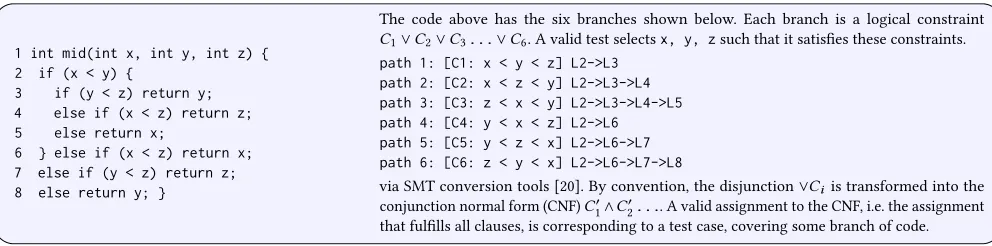
1 int mid(int x, int y, int z) { 2 if (x < y) {
3 if (y < z) return y; 4 else if (x < z) return z; 5 else return x;
6 } else if (x < z) return x; 7 else if (y < z) return z; 8 else return y; }
The code above has the six branches shown below. Each branch is a logical constraint C1_C2_C3. . ._C6. A valid test selectsx, y, zsuch that it satis�es these constraints. path 1: [C1: x < y < z] L2->L3
path 2: [C2: x < z < y] L2->L3->L4 path 3: [C3: z < x < y] L2->L3->L4->L5 path 4: [C4: y < x < z] L2->L6 path 5: [C5: y < z < x] L2->L6->L7 path 6: [C6: z < y < x] L2->L6->L7->L8
via SMT conversion tools [20]. By convention, the disjunction_Ci is transformed into the conjunction normal form (CNF)C0
1^C02. . .. A valid assignment to the CNF, i.e. the assignment that ful�lls all clauses, is corresponding to a test case, covering some branch of code.
Figure 1: A script of C programming can be translated into CNF form, the target problem discussed in this paper.
That is, backdoors are a way to turn very slow exponential time tasks into much faster polynomial-time tasks. Numerous studies have con�rmed the existence of such backdoors, in many domains[2, 4, 31, 36]. Fichteet al.[19] proposed backdoor-based methods to solve the answer set programming problem (ASP), i.e. the search for answer sets in disjunctive logic programs. Up to then, the most successful solvers for disjunctive ASP [23] were based on SAT techniques and the concept of loop formulas [30]. Fichteet al. ex-ploited the small distance of a disjunctive program from being normal (such distance is measured in terms of the size the smallest backdoor to normality, i.e. the smallest number of atoms whose deletion makes the program normal). Among the structured (i.e. non-random) domains, experiments showed that only 1 to 10% of atoms were included in the smallest strong backdoors. Also, Kro-neggeret al.[29] proposed an algorithm to�lter the backdoors for planningproblem. Their “backdoors for planning” method built upon the so-called causal graph. Such graphs model the dependen-cies between variables in planning instances. Based on the structure of the causal graph, various tractable fragments of planning can be identi�ed. The algorithm contains two phases: 1) the detection phase –�nding the small backdoor and 2) the evaluation phase – using the additional information given in the backdoor to solve the planning instance.
The above works show that a small ratio (<10%) of variables, i.e. the backdoors, did signi�cantly reduce the complexity of the SE models. But showing that the backdoors exist is a di�erent question to “how to�nd the backdoors, quickly”. Fichte and Kronegger etc.’s methods are not optimized to reduce CPU cost or minimize the size of the returned model (which are two properties that we desire in test suites). What’s more, their algorithms are not simple to understand and implement, due to the somewhat arcane and tricky nature of their lemmas and propositions.
2.2 Theorem Proving in Software Testing
This section describes some of the ways software testing can be recast as a theorem proving problem. Note that, once recast in this way, SAT solvers can be used as test case generation tools.
Aritoet al.proposed a framework to transform the test suite min-imization problem (TSMP) in regression testing into a constrained SAT problem [3]. This transformation is done by modeling TSMP instances as a set of Pseudo-Boolean constraints that are later trans-lated to SAT instances. TSMP has two objectives: 1) minimizing the
testing cost and 2) maximizing the program coverage. To start with, a set of test casesT={t1,t2,t3, . . .}as well as their running time cost{c1,c2, . . .}is de�ned.
•ti is a binary signal indicating if the test caseishould be tested.
• The information about whether test caseti covers some element in the programej is stored as the binary matrix M=[mij].
To translate the TSMP into constrained problems, we have all fol-lowing pseudo-boolean constraints:Õn
i=1citi BandÕmj=1ej P
whereB 2Zis the maximum allowed cost andP 2{1,2, . . . ,m} is the minimum coverage level. Having the pseudo-boolean con-straints, Eenet al.[16] provides three techniques to translate pseudo-boolean constraints (linear constraints over pseudo-boolean variables) into clauses that can be handled by a SAT-solver.
As another scenario, combinatorial testing [38] can be expressed in the form of conjunctive normal form (CNF) and hence studied by a SAT solver. Combinatorial testing covers interactions of parame-ters in the system under test. A well-chosen sampling mechanism can reduce the cost of software and system testing by reducing the number of test cases to be executed [44]. Considering the sys-tem environment {AMD, Intel}⇥{Windows, MacOS, Linux}⇥{IE, Firefox, Safari}. Note that not all combinations valid. For example, MacOS does not support AMD processor while IE does not support MacOS, etc. All of such constraints can be expressed as the feature model [27] or as product lines. Further, such a feature model can be transformed into the CNF formulas [35], at which point, SAT solvers can compute out the valid testing environment combination. Last but not least, given a script of C programming, one can trans-late it into CNF formulas, as done in Figure 1. Symbolic/dynamic execution techniques [5, 12] extract the possible execution branches of a procedural program. Each branch is a conjunction of conditions Bi=Cx^C ^...so the whole program can be summarized as the disjunctionBi_Bj_.... Using deMorgan’s rules2these clauses can be converted to conjunctive normal form (CNF) where the inputs to the program are the variables in the CNF.
2Disjunctions to conjunctions:P_Q⌘(¬P^¬Q)
393 394 395 396 397 398 399 400 401 402 403 404 405 406 407 408 409 410 411 412 413 414 415 416 417 418 419 420 421 422 423 424 425 426 427 428 429 430 431 432 433 434 435 436 437 438 439 440 441 442 443 444 445 446 447 448 449 450
451 452 453 454 455 456 457 458 459 460 461 462 463 464 465 466 467 468 469 470 471 472 473 474 475 476 477 478 479 480 481 482 483 484 485 486 487 488 489 490 491 492 493 494 495 496 497 498 499 500 501 502 503 504 505 506 507 508 509 510 511 512 513 514 515 516 517 518 519 520 521 522 523 524 525 526 527 528 529 530
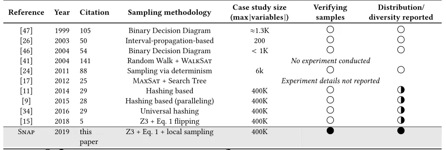
Table 1:S���and its related work for solving theorem proving constraints via sampling.
Reference Year Citation Sampling methodology (maxCase study size|variables|) Verifyingsamples diversity reportedDistribution/
[47] 1999 105 Binary Decision Diagram ⇡1.3K [26] 2003 50 Interval-propagation-based 200 [46] 2004 54 Binary Decision Diagram <1K
[41] 2004 141 Random Walk +W���S�� No experiment conducted [24] 2011 88 Sampling via determinism 6k
[17] 2012 25 M��S��+ Search Tree Experiment details not reported
[11] 2014 29 Hashing based 400K
[9] 2015 28 Hashing based (paralleling) 400K [34] 2016 29 Universal hashing 400K [15] 2018 5 Z3 + Eq. 1�ipping 400K S��� 2019 this
paper Z3 + Eq. 1 + local sampling 400K
/ : the absence / presence of corresponding item : only partial case studies(the small case studies)were reported
2.3 Theorem Prover Research in SE
As shown in Table 1, much prior research has explored scaling theorem proving for software engineering. One way to tame the theorem proving problem is to simplify or decompose the CNF formulas. A recent example in this arena wasGreenTire, proposed by Jiaet al.[28].GreenTiresupports constraint reuse based on the logical implication relation among constraints. One advantage of this approach is its e�ciency guarantees. Similar to the analyti-cal methods in linear programming, they are always applied to a speci�c class of problem. However, even with the improved theo-rem prover, such methods may be di�cult to be adopted in large models.GreenTirewas tested in 7 case studies. Each case study was corresponding to a small code script with ten lines of code, e.g. the BinTreein [40]. For the larger models, such as those explored in this paper, the following methods might do better.
Another approach, which we will call sampling, is to combine theorem provers Z3 with stochastic sampling heuristics. For exam-ple, given random selections forb,c, Eq. 1 might be used to generate a new test suite, without calling a theorem prover. Theorem proving might then be applied to some (small) subset of the newly generated tests, just to assess how well the heuristics are working.
The earliest sampling tools were based on binary decision dia-grams (BDDs) [1]. Yuanet al.[46, 47] build a BDD from the input constraint model and then weighted the branches of the vertices in the tree such that a stochastic walk from root to the leaf was able to generate samples with the desired distribution. In other work, Iyer proposed a technique namedRACEwhich has been applied in multiple industrial solutions [26].RACE(a) builds a high-level model to represent the constraints; then (b) implements a branch-and-bound algorithm for sampling diverse solutions. The advantage ofRACEis its implementation simplicity. However,RACE, as well as the BDD-based approached introduced above, return highly biased samples, that is, highly non-uniform samples. For testing, this is not recommended since it means small parts of the code get explored at a much higher frequency than others.
Using a SAT solverWalkSat[39], Weiet al.[41] proposed Sam-pleSAT.SampleSATcombines random walk steps with greedy steps
fromWalkSat– a method that works well for small models. However, due to the greedy nature ofWalkSat, the performance ofSampleSAT is highly skewed as the size of the constraint model increases.
For seeking diverse samples, universal hashing [33] techniques have been proposed. These algorithms were designed for strong guarantees of uniformity. Meelet al.[34] provided an overview of key ingredients of integration of universal hashing and SAT solvers; e.g. with universal hashing, it is possible to guarantee uni-form solutions to a constraint model. These hashing algorithms can be applied to the extreme large models (with near 0.5M vari-ables). More recently, several improved hashing-based techniques have been purposed to balance the scalability of the algorithm as well as diversity (i.e. uniform distribution) requirements. For exam-ple, Chakrabortyet al.proposed an algorithm namedUniGen[11], following by theUnigen2[9].UniGenprovides strong theoretical guarantees on the uniformity of generated solutions and has ap-plied to constraint models with hundreds of thousands of variables. However,UniGensu�ered from a large computation resource re-quirement. Later work explored a parallel version of this approach. Unigen2achieved near linear speedup of the number of CPU cores. To the best of our knowledge, the state-of-the-art technique for generating test cases using theorem provers isQuickSampler[15]. QuickSamplerwas evaluated on large real-world case studies, some of which have more than 400K variables. At ICSE’18, it was shown thatQuickSampleroutperforms aforementionedUnigen2as well as another similar technique namedSearchTreeSampler[17]. Quick-Samplerstarts from a set of valid solutions generated by Z3. Next, it computes the di�erences between the solutions using Eq. 1. New test cases generated in this manner are not guaranteed to be valid. QuickSamplerde�nes three terms, we use later in this paper:
• A test suite is a set of valid tests.
• A test isvalidif uses input settings that satisfy the CNF. • One test suite is morediversethan another if it uses more
variable within the CNF disjunctions.Diversetest suites are preferred since they cover more parts of the code.
531 532 533 534 535 536 537 538 539 540 541 542 543 544 545 546 547 548 549 550 551 552 553 554 555 556 557 558 559 560 561 562 563 564 565 566 567 568 569 570 571 572 573 574 575 576 577 578 579 580 581 582 583 584 585 586 587 588
589 590 591 592 593 594 595 596 597 598 599 600 601 602 603 604 605 606 607 608 609 610 611 612 613 614 615 616 617 618 619 620 621 622 623 624 625 626 627 628 629 630 631 632 633 634 635 636 637 638 639 640 641 642 643 644 645 646 647 648 649 650 651 652 653 654 655 656 657 658 659 660 661 662 663 664 665 666 667 668
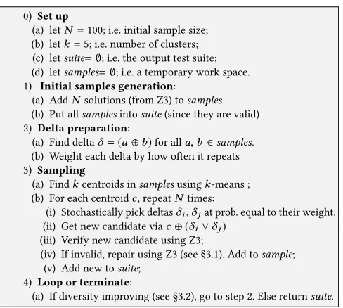
0) Set up
(a) letN=100; i.e. initial sample size;
(b) letk=5; i.e. number of clusters;
(c) letsuite=;; i.e. the output test suite;
(d) letsamples=;; i.e. a temporary work space.
1) Initial samples generation:
(a) AddNsolutions (from Z3) tosamples (b) Put allsamplesintosuite(since they are valid)
2) Delta preparation:
(a) Find delta =(a b)for alla,b2samples. (b) Weight each delta by how often it repeats
3) Sampling
(a) Findkcentroids insamplesusingk-means ; (b) For each centroidc, repeatNtimes:
(i) Stochastically pick deltas i, jat prob. equal to their weight. (ii) Get new candidate viac ( i_ j)
(iii) Verify new candidate using Z3;
(iv) If invalid, repair using Z3 (see §3.1). Add tosample; (v) Add new tosuite;
4) Loop or terminate:
(a) If diversity improving (see §3.2), go to step 2. Else returnsuite.
Figure 2:S���
valid tests found byS���, on the other hand, is 100%. Further, as shown below,S���builds those tests with enough diversity much faster thanQuickSampler.
3 IMPLEMENTING THE
SNAP
TACTIC
In theS���algorithm if Figure 2, each test is a set of zeros or ones (false, true) assigned to all the variables in a CNF formula.
As shown ininitial samples(steps 1a,1b), instead of computing some deltas between many tests,S���restrains mutation to the deltas between a few valid tests (generated from Z3).S���builds a pool of 10,000 deltas fromN =100valid tests (which mean calling a theorem prover onlyN =100times).S���uses this pool as a set of candidate “mutators” for existing tests (and by “mutator”, we mean an operation that converts an existing test into a new one).
After that, indelta preparation(steps 2a,2b),S���applies Eq. 1. Note that the more often a setting repeats, the more likely it is a backdoor variable. Hence, step 2b sorts the deltas on occurrence frequency. This sort is used in step 3b.
Insample(steps 3a,3b),S����samples around the average val-ues seen in a few randomly selected valid tests. Here, "averaging" is inferred by using the median values seen inkclusters. Note that, in step 3b, we use deltas that are more likely to be backdoor variables (i.e. we use the deltas that occur more frequently).
Step 3b.ii is where we verify the new candidate using Z3.S���
explores far fewer candidates thanQuickSampler(10 to 750 times fewer, see §5.3). Since we are exploring less, we can take the time to verify them all. Hence, 100% ofS���’s tests are valid (and the same isnottrue forQuickSampler– see §5.1).
Note that in 3b.iv, if a candidate passes veri�cation, we output it then forget about it. Else, we repair it and add it to our clusters. We do this since test cases that pass veri�cation do not add new infor-mation to our samples. However, when an instance fails veri�cation and is repaired, that o�ers new settings.
Note also thatS���takes great care in how it calls a theorem prover. Theorem provers are much slower forgeneratingnew tests thanrepairinginvalid tests than forverifyingthat a test is valid (since there are more options for generation that for repairing than for veri�cation). Hence,S���needs toverifymore than itrepairs (and also dorepairsmore thangeneratingnew tests). Accordingly, The call to Z3 in step 1a can be the slowest (since this agenerate call that must navigate all the constraints of our CNF). Hence, we only do thisN =100times. Also, the call to Z3 in step 3b.iii is a veri�cation calland is much faster since all the variables are set. Finally, The call of Z3 in the step 3b.ivrepaircall, is slower than step 3b.iii since (as discussed below), our repair operator introduces some open choices into the test. Note that we only need to repair the small minority of new tests that fail veri�cation. Later in this paper, we can use Figure 4 to show that repairs are only needed on 30% (median) of all tests.
3.1 Implementing “Repair”
S���’s repair function deletes “dubious” parts of a test case, then uses Z3 to�ll in the the gaps. In this way, when we repair a test, most bits are set and Z3 only has to search a small space.
To�nd the “dubious” section, we re�ect on how step 3b.ii oper-ates. Recall that the new test uses =a banda,bare valid tests taken fromsamples. Sincea,bwere valid, then the “dubious” parts of the test is anything that was not seen in bothaandb. Hence, we preserve the bits inc bits (where the corresponding bit was 1), while removing all other bits (where bit was 0). For example: • When mutatingc=(1,0,0,1,1,0,0,0) using =(1,0,1,0, 1,0,1,0). • Ifc =(0,0,1,1,0,0,1,0) is invalid, thenS���deletes the
“dubious” sections as follows.
• S���preserves any “1” bits that were seen in .
• S���deletes the others; e.g. bits 2, 4, 6, 8 (0,A0,1,A1,0,A0, 1,A0). • Z3 is then called to�ll out the missing bits of(0?1?0?1?).
3.2 Implementing “Termination”
To implementS���’s termination criteria (step 4a), we need a work-ing measure of diversity. Recall from the introduction that one test suite is morediversethan another if it uses more of the variable settings with disjunctions inside the CNF.Diversetest suites are bettersince they cover more parts of the code.
To measure diversity, we used Feldtet al.[18]’s normalized com-pression distance (NCD). A test suite with high NCD implies higher code coverage during the testing3. NCD usesgzipto the estimate Kolmogorov complexity [32] of the tests. IfC(x)is the length of compression ofx andC(X)is the compression length of binary string setX’s concatenation, then:
NCD(X)=C(X) minx2X{C(x)}
maxx2X{C(X\{x})} (2)
S���exits if NCD improves byX 5%in the lastT =10minutes.
3.3 Engineering Choices
S���uses theses control parameters (set via engineering judgment):
3Aside: we note that we did not adopt the diversity metric (distribution of samples
669 670 671 672 673 674 675 676 677 678 679 680 681 682 683 684 685 686 687 688 689 690 691 692 693 694 695 696 697 698 699 700 701 702 703 704 705 706 707 708 709 710 711 712 713 714 715 716 717 718 719 720 721 722 723 724 725 726
727 728 729 730 731 732 733 734 735 736 737 738 739 740 741 742 743 744 745 746 747 748 749 750 751 752 753 754 755 756 757 758 759 760 761 762 763 764 765 766 767 768 769 770 771 772 773 774 775 776 777 778 779 780 781 782 783 784 785 786 787 788 789 790 791 792 793 794 795 796 797 798 799 800 801 802 803 804 805 806 •X =5%;
•T =10minutes; •N =100samples; •k=5clusters.
In future work, it could be insightful to vary these values. Another area that might bear further investigation is the clus-tering method used in step 3a. For this paper, we tried di�erent clustering methods. Clustering ran so fast that we were not mo-tivated to explore alternate algorithms. Also, we found that the details of the clustering were less important than pruning away most of the items within each cluster (so that we only mutate the centroid).
4 EXPERIMENTAL SET-UP
4.1 Code
To explore the research questions shown in the introduction, the
S���system shown in Algorithm 2 was implemented in C++ using Z3 v4.8.4 (the latest release when the experiment was conducted). Ak-means cluster was added using the free edition of ALGLIB [7], a numerical analysis and data processing library delivered for free under GPL or Personal/Academic license.QuickSamplerdoes not integrate the samples veri�cation into the work�ow. Hence, in the experiment, we adjusted the work�ow ofQuickSamplerso that all samples are veri�ed before termination. Also, the outputs of QuickSamplerwere the assignments of independent support. The independent supportis a subset of variables which completely deter-mines all the assignments to a formula [15]. In practice, engineers need the complete test case input; consequently, for valid sam-ples, we extended theQuickSamplerto get full assignments of all variables from independent support’s assignment via propagation.
4.2 Experimental Rig
We comparedS���to the state-of-the-artQuickSampler, technique purposed by Dutraet al.at ICSE’18. To ensure a repeatable result, we updated the Z3 solver inQuickSamplerinto the latest version.
To reduce the observation error and test the performance ro-bustness, we repeated all experiment 30 times with 30 di�erent random seeds. To simulate real practice, such random seeds were used in Z3 solver (for initial solution generation), ALGLIB (for the k-means) and other components. Due to the space limitation, we cannot report results for all 30 repeats. Correspondingly we report the medium or the IQR (75-25th variations) results.
All experiments were conducted on Xeon-E5@2GHz machines with 4GB memory, running CentOS. These were multi-core ma-chines but for systems reasons, we only used one core per machine.
4.3 Case Studies
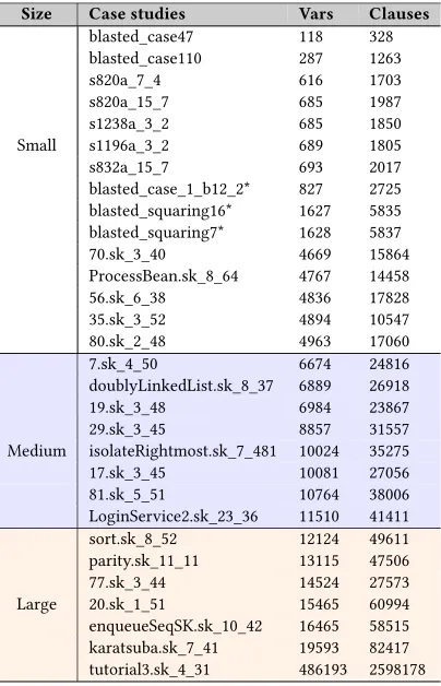
Table 2 lists the case studies used in this work. We can see that the number of variables ranges from hundreds to more than 486K. The large examples have more than 50K clauses, which is very huge. For exposition purposes, we divided the case studies into three groups: the small case studies with vars<6K; the medium case studies with6K<vars<12Kand the large case studies with vars>12K. For the following reasons, our case studies are the same as those used in theQuickSamplerpaper:
Table 2: Case studies used in this paper. Sorted by number of variables. Medium sized-problems are highlighted withblue rowswhile the large ones are inorange rows. Three items (marked with *) are not included in some further reports (see text). See text for details.
Size Case studies Vars Clauses
blasted_case47 118 328 blasted_case110 287 1263
s820a_7_4 616 1703
s820a_15_7 685 1987
s1238a_3_2 685 1850
Small s1196a_3_2 689 1805
s832a_15_7 693 2017
blasted_case_1_b12_2* 827 2725 blasted_squaring16* 1627 5835 blasted_squaring7* 1628 5837 70.sk_3_40 4669 15864 ProcessBean.sk_8_64 4767 14458 56.sk_6_38 4836 17828 35.sk_3_52 4894 10547 80.sk_2_48 4963 17060
7.sk_4_50 6674 24816
doublyLinkedList.sk_8_37 6889 26918 19.sk_3_48 6984 23867 29.sk_3_45 8857 31557 Medium isolateRightmost.sk_7_481 10024 35275 17.sk_3_45 10081 27056 81.sk_5_51 10764 38006 LoginService2.sk_23_36 11510 41411 sort.sk_8_52 12124 49611 parity.sk_11_11 13115 47506 77.sk_3_44 14524 27573 Large 20.sk_1_51 15465 60994 enqueueSeqSK.sk_10_42 16465 58515 karatsuba.sk_7_41 19593 82417 tutorial3.sk_4_31 486193 2598178
• We wanted to compare our method toQuickSampler; • Their case studies were online available;
• Their case studies are used in multiple papers [9, 11, 15, 34] etc.
These case studies are representative of scenarios engineers met in software testing or circuit testing in embedded system design. They include bit-blasted versions of SMTLib case studies, ISCAS89 circuits augmented with parity conditions on randomly chosen subsets of outputs and next-state variables, problems arising from automated program synthesis and constraints arising in bounded theorem proving. For more introduction of the case studies, please see [9, 15].
For pragmatic reasons, certain case studies were omitted from our study. For example, we do not report ondiagStencilClean.sk_41_36 in the experiment since the purpose of this paper is to sample a set of valid solutions to meet the diversity requirement; while there are only 13 valid solutions from this model. TheQuickSamplerspent 20 minutes (on average) to search for one solution.
807 808 809 810 811 812 813 814 815 816 817 818 819 820 821 822 823 824 825 826 827 828 829 830 831 832 833 834 835 836 837 838 839 840 841 842 843 844 845 846 847 848 849 850 851 852 853 854 855 856 857 858 859 860 861 862 863 864
865 866 867 868 869 870 871 872 873 874 875 876 877 878 879 880 881 882 883 884 885 886 887 888 889 890 891 892 893 894 895 896 897 898 899 900 901 902 903 904 905 906 907 908 909 910 911 912 913 914 915 916 917 918 919 920 921 922 923 924 925 926 927 928 929 930 931 932 933 934 935 936 937 938 939 940 941 942 943 944
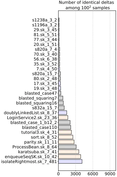
Figure 3: Number of identical deltas among 100*100 pair of valid solution deltas for all case studies. Same color scheme as Table 2.
QuickSamplergenerates tens of millions of samples for these exam-ples, all samples were the assignment to theindependent support (de�ned in §4.1). The omission of these case studies is not a critical issue. Solving or sampling these examples is not di�cult; since they are all very small, as compared to other larger case studies.
5 RESULTS
The rest of this paper use the machinery de�ned above to answer the four research questions posed in the introduction. Before answering those questions, we o�er one negative result. Table 2 color-coded our case studies such that the medium to large case studies is shown in blue and orange. Looking across all the following results, with the exception of runtimes, we see no pattern in the color coding (e.g. it isnottrue that larger problems have more duplicates). From this lack-of-pattern, we conclude that the complexity of test suite generation comes from the relationships between the variables, and not necessarily the number of variables themselves.
5.1 RQ1: How Reliable is the Eq. 1 Heuristic?
QuickSamplerran quickly since it assumed that tests generated using Eq. 1 did not need veri�cation. To check that assumption, for each case study, we randomly generated 100 valid solutions, S={s1,s2, . . .s100}using Z3. Next, we selected three{a,b,c}2S and built a new test case using Eq. 1; i.e.new=c (a b).Figure 4: RQ1 results: percentage of valid mutations found it step3b.iii (computed separately for each case study).
Figure 3 lists the number of identical deltas seen in1002of those deltas. Among all case studies, we rarely found large sets of unique deltas. Hence, among the 100 valid solutions given by Z3, many s were shared within pairwise solutions. This is important since if otherwise, the Eq. 1 heuristic would be dubious.
The percentage of these deltas that proved to be valid in step3b.iii of Algorithm 1 are shown in Figure 4. Dutraet al.’s estimate was that the percentage of valid tests generated by Eq. 1 was usually 70% or more. As shown by the median values of Figure 4, this was indeed the case. However, we also see that in the lower third of those results, the percent of valid tests generated by Eq. 1 is very low: 25% to 50% (median to max). This result alone would be enough to make us cautious about usingQuickSamplersince, when the Eq. 1 heuristics fails, it seems to fail very badly. We recommend:
Conclusion #1: Eq. 1 should not be used without veri�cation of the resulting test.
By way of comparisons, it is useful to add here thatS���veri�es every test case it generates. This is practical forS���, but imprac-tical forQuickSamplersince these two systems typically process 102to108test cases, respectively. In any case, another reason to recommendS���is that this tool delivers tests suites where 100% of all tests are valid.
5.2 RQ2: How Fast is
S���
?
Figure 5 shows the execution time required forS���and Quick-Sampler. The y-axis of this plot is a log-scale and shows time in seconds. These results are shown in the same order as Table 2. That is, from left to right, these case studies grow from around 300 to around 3,000,000 clauses.
For the smaller case studies, shown on the left,S���is sometimes slower thanQuickSampler. Moving left to right, from smaller to larger case studies, it can be seen thatS���often terminates much faster thanQuickSampler. On the very right-hand side of Figure 5, there are some results where is seemsS���is not particularly fastest. This is due to the log-scale applied to the y-axis. Even in these cases,
S���is terminating in less than our while other approaches need more than two hours.
Figure 6 is a summary of Figure 5 that divides the execution time for both systems. From this�gure it can be seen:
945 946 947 948 949 950 951 952 953 954 955 956 957 958 959 960 961 962 963 964 965 966 967 968 969 970 971 972 973 974 975 976 977 978 979 980 981 982 983 984 985 986 987 988 989 990 991 992 993 994 995 996 997 998 999 1000 1001 1002
1003 1004 1005 1006 1007 1008 1009 1010 1011 1012 1013 1014 1015 1016 1017 1018 1019 1020 1021 1022 1023 1024 1025 1026 1027 1028 1029 1030 1031 1032 1033 1034 1035 1036 1037 1038 1039 1040 1041 1042 1043 1044 1045 1046 1047 1048 1049 1050 1051 1052 1053 1054 1055 1056 1057 1058 1059 1060 1061 1062 1063 1064 1065 1066 1067 1068 1069 1070 1071 1072 1073 1074 1075 1076 1077 1078 1079 1080 1081 1082
Figure 5: RQ3 results: Time to terminated (seconds), The y-axis is in log scale. TheS���sampling time fors1238_a_3_2and
parity.sk_11_11is not reported since their achieved NCD were much worse thanQuickSampler’s (see Figure 7). Figure 6 illustrates the corresponding speedups.
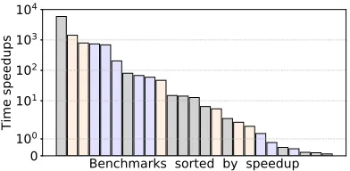
Figure 6: RQ2 results: Sortedspeedup(time(QuickSampler) / time(S���)). If over100, thenS���terminates earlier.
Conclusion #2: S���was 10 to 3000 times faster than Quick-Sampler(median to max).
There are some exceptions to this conclusion, where QuickSam-plerwas faster thanS���(see the right-hand-side of Figure 6). Those cases are usually for small models (17,000 clauses or less). For medium to larger models, with 20,000 to 2.5 million clauses,
S���is often orders of magnitude faster.
5.3 RQ3: How Easy is it to Apply
S���
’s Test
Cases?
Table 3 compares the number of tests fromQuickSamplerandS���. As shown by the last column in that table:
Conclusion #4: S���’s test cases were 10 to 750 times smaller than those ofQuickSampler(median to max).
Hence we say that usingS���is easier than other methods, where “easier” is de�ned as per ourIntroduction. That is, when test suites
are 10 to 750 times smaller, then they are faster to run, consumes less cloud-compute resources, and means developers have to spend less time processing failed tests.
5.4 RQ4: How Diverse are the
S���
Test Cases?
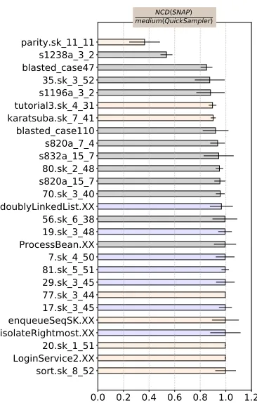
Figure 7 compares the diversity of the test suites generated by our two systems. These results are expressed as ratios of the observed NCD values. Results less than one indicate thatS���’s test suites are less diverse thanQuickSampler. In the median case, the ratio is one; i.e. in terms of central tendency, there is no di�erence between the two algorithms.
We have analyzed the Figure 7 results with a bootstrap test at 95% con�dence (to test for statistically signi�cant results), and a Cohen’s e�ect size test (to rule out trivially small di�erences). Based on those tests, we say that in 2025 = 80%of these results, there is no signi�cant di�erence (of non-trivial size) between the two algorithms. Further, in two cases where there was a statistical di�erence (tutorial2,sk_4_31 and karatsuba_sk_7_41) the di�erence is less than 10%. Pragmatically, we argue that such a small di�erence is not troubling. Hence, we say:
Conclusion #4: The diversity ofS���’s test suites is very similar to those ofQuickSampler.
That said, there are two examples whereS����’s diversity is markedly less than one (see s1238a_3_2 and parity.sk_11_11). In terms of scoring di�erent algorithms, it could be argued that these examples might mean thatQuickSampleris the preferred algorithm but only (a) if numerous invalid tests are not an issue; (b) if testing resources are fast and cheap (so saving time and money on cloud-compute test facilities is not worthwhile); and (c) if developer time is cheap (so the time required to specify expected test output, or processing large numbers of failed tests, is not an issue).
1083 1084 1085 1086 1087 1088 1089 1090 1091 1092 1093 1094 1095 1096 1097 1098 1099 1100 1101 1102 1103 1104 1105 1106 1107 1108 1109 1110 1111 1112 1113 1114 1115 1116 1117 1118 1119 1120 1121 1122 1123 1124 1125 1126 1127 1128 1129 1130 1131 1132 1133 1134 1135 1136 1137 1138 1139 1140
1141 1142 1143 1144 1145 1146 1147 1148 1149 1150 1151 1152 1153 1154 1155 1156 1157 1158 1159 1160 1161 1162 1163 1164 1165 1166 1167 1168 1169 1170 1171 1172 1173 1174 1175 1176 1177 1178 1179 1180 1181 1182 1183 1184 1185 1186 1187 1188 1189 1190 1191 1192 1193 1194 1195 1196 1197 1198 1199 1200 1201 1202 1203 1204 1205 1206 1207 1208 1209 1210 1211 1212 1213 1214 1215 1216 1217 1218 1219 1220
Table 3: RQ3: results. Number of unique valid cases in test suite. Sorted by last column. Same color scheme as Table 2.
SS SQ SQ/ Case studies S��� QuickSampler SS
blasted_case47 2899 71 0.02
isolateRightmost 15480 7510 0.49
LoginService2 404 210 0.52
19.sk_3_48 204 200 0.98
70.sk_3_40 3050 4270 1.40
s820a_15_7 29065 70099 2.41
29.sk_3_45 225 660 2.93
s820a_7_4 37463 124457 3.32
s832a_15_7 27540 96764 3.51
s1196a_3_2 225 1890 8.40
enqueueSeqSK 338 2495 7.38
blasted_case110 274 2386 8.71
tutorial3.sk_4_31 336 2953 8.79
81.sk_5_51 227 2814 12.40
sort.sk_8_52 812 10184 12.54
karatsuba.sk_7_41 139 4210 30.29
20.sk_1_51 239 10039 42.00
doublyLinkedList 278 12042 43.32
17.sk_3_45 228 12780 56.05
ProcessBean 1193 75392 63.20
7.sk_4_50 258 18090 70.12
56.sk_6_38 1827 149031 81.57
80.sk_2_48 653 54440 83.37
77.sk_3_44 245 33858 138.20
35.sk_3_52 258 193920 751.63
We note that such an argument is orthogonal to the goals of this paper. Our goal is to suggest that SE tasks that use propositional theorem provers can bene�t from phenomena reported in the AI literature; i.e. the backdoor e�ect. As evidence of that bene�t, we point to (1) the brevity ofS���’s tests; (2) the speed with which they can be generated and fully veri�ed, and (3) their similar diversity.
6 THREATS TO VALIDITY
One threat to the validity of this work is thebaseline bias. Indeed, there are many other sampling techniques, or solvers, thatS���
might be compared to. However, our goal here was to compare
S���to a recent state-of-the-art result from ICSE’18. In further work, we will compareS���to other methods.
A second threat to validity isinternal biasthat raises from the sto-chastic nature of sampling techniques.S���requires many random operations. To mitigate the threats, we repeated the experiments for 30 times and reported the medium or IQR of those results.
A third threat is themeasurement bias. To determine the diversity of a test suite, in the experiment, we use normalized compression distance (NCD). Prior research has argued for the value of that mea-sure [18]. However, there exist many other diversity meamea-surements for the theorem proving problem, such as [10], and changing the diversity measurement might lead to a change of the results. That said, in one research report, it is impossible to explore all options.
Figure 7: RQ4 results: Normalized compression distance (NCD) f or when QuickSampler and S��� terminated on the same case studies. Median results over 30 runs (and small black lines show the 75th-25th variations). Same color scheme as Table 2.
For the convenient of further exploration, we have released the source code ofS���in the hope that other researchers will assist us by evaluatingS���on a broader range of measures.
Another threat ishyperparameter bias. The hyperparameter is the set of con�gurations for the algorithm. There now exists a range of mature hyperparameter optimizers [21, 37, 43] which might be useful for�nding better settings forS���. This is a clear direction for future work.
Finally, as toconstruct validity, this paper argued for the bene�t of backdoors by analyzing the di�erence between two algorithms:
S���andQuickSampler. For that purpose, we usedQuickSampler exactly as it was described in its ICSE’18 paper. Note that a case could be made to “tinker” withQuickSamplerin order to, say, use a di�erent termination condition. We did not do that since there are many ways we could tinker withQuickSamplerusing di�erent parts of Figure 2. For example, tinkering could add delta mutation, or clustering, or our repair algorithm– at which point we would not be compared against theQuickSampleralgorithm of ICSE’18 but some other algorithm of our own invention. For future work, we are exploring many of those “tinkerings”. But for this paper, which is a baseline result commenting on the bene�t of backdoor-based reasoning, our current approach is more justi�able.
1221 1222 1223 1224 1225 1226 1227 1228 1229 1230 1231 1232 1233 1234 1235 1236 1237 1238 1239 1240 1241 1242 1243 1244 1245 1246 1247 1248 1249 1250 1251 1252 1253 1254 1255 1256 1257 1258 1259 1260 1261 1262 1263 1264 1265 1266 1267 1268 1269 1270 1271 1272 1273 1274 1275 1276 1277 1278
1279 1280 1281 1282 1283 1284 1285 1286 1287 1288 1289 1290 1291 1292 1293 1294 1295 1296 1297 1298 1299 1300 1301 1302 1303 1304 1305 1306 1307 1308 1309 1310 1311 1312 1313 1314 1315 1316 1317 1318 1319 1320 1321 1322 1323 1324 1325 1326 1327 1328 1329 1330 1331 1332 1333 1334 1335 1336 1337 1338 1339 1340 1341 1342 1343 1344 1345 1346 1347 1348 1349 1350 1351 1352 1353 1354 1355 1356 1357 1358
7 CONCLUSION
Exploring propositional formula is a core computational process with many areas of application. Here, we explore the use of such formula for test suite generation. SAT solvers are a promising tech-nology for�nding settings that satisfy propositional formula. The current generation of SAT solvers is challenged by the size of the formula seen in the recent SE testing literature.
One tactic for taming the computational complexity of SAT solv-ing is the backdoor e�ect. AI researchers report that when propo-sitional formula share many settings, then fast solutions can be generated by�rst setting just a few of those variables. The goal of this paper was to test the e�cacy of such backdoor-based reasoning. To the best of our knowledge, this is the�rst paper to�nd, and successfully exploit, backdoor e�ects in SE testing.
TheS���algorithm was an experiment to apply backdoors to software testing. We reasoned that the common settings seen in a smallMsample of valid tests may also be the common settings in a largeN Msample. If so, then test case generation could be made faster by sampling around the average values seen in a few randomly selected valid tests.
Experiments withS���are strongly supportive of the bene�ts of backdoors for SE tasks. On experimentation, we found that when this tactic was applied to 27 real-world test case studies,S���ran 10 to 3000 times faster (median to max) than a prior report (reported at ICSE’18). While that prior work found tests that were 70% valid, SNAP’s generated 100% valid tests. Another important result was the size of the test set generated via backdoor-reasoning. There is an economic imperative to run fewer tests when companies have to pay money to run each test, and when developers have to spend time studying the failed test. In that context, it is interesting to note that SNAP’s tests are 10 to 750 times smaller (median to max) than those from prior work.
In future work, we want to see if backdoors help other SE tasks that use propositional formula. For example, all the formula here have yes, no answers. Another kind of task areoptimizersthat explore satis�cing trade-o�s between competing constraints. To that end, we are currently working on applying backdoors to the vZ [6] optimizing theorem prover.
REFERENCES
[1] Sheldon B. Akers. 1978. Binary decision diagrams.IEEE Trans. Computers6 (1978), 509–516.
[2] Carlos Ansótegui, Jesús Giráldez-Cru, and Jordi Levy. 2012. The community structure of SAT formulas. InTAST. Springer, 410–423.
[3] Franco Arito, Francisco Chicano, and Enrique Alba. 2012. On the application of SAT solvers to the test suite minimization problem. InSSBSE. Springer, 45–59. [4] Gilles Audemard and Laurent Simon. 2009. Predicting learnt clauses quality in
modern SAT solvers. InIJCAI.
[5] Roberto Baldoni, Emilio Coppa, Daniele Cono DâĂŹelia, Camil Demetrescu, and Irene Finocchi. 2018. A survey of symbolic execution techniques. ACM Computing Surveys (CSUR)51, 3 (2018), 50.
[6] Nikolaj Bjørner, Anh-Dung Phan, and Lars Fleckenstein. 2015. Z-an optimizing SMT solver. InInternational Conference on Tools and Algorithms for the Construc-tion and Analysis of Systems. Springer, 194–199.
[7] Sergey Bochkanov and Vladimir Bystritsky. 2013. Alglib.Available from: www. alglib. net59 (2013).
[8] Roberto Bruttomesso, Alessandro Cimatti, Anders Franzén, Alberto Griggio, and Roberto Sebastiani. 2008. The mathsat 4 smt solver. InInternational Conference on Computer Aided Veri�cation. Springer, 299–303.
[9] Supratik Chakraborty, Daniel J Fremont, Kuldeep S Meel, Sanjit A Seshia, and Moshe Y Vardi. 2015. On parallel scalable uniform SAT witness generation. In International Conference on Tools and Algorithms for the Construction and Analysis of Systems. Springer, 304–319.
[10] Sourav Chakraborty and Kuldeep S. Meel. 2019. On testing of Uniform Samplers. InProceedings of AAAI Conference on Arti�cial Intelligence (AAAI).
[11] Supratik Chakraborty, Kuldeep S Meel, and Moshe Y Vardi. 2014. Balancing scalability and uniformity in SAT witness generator. InProceedings of the 51st Annual Design Automation Conference. ACM, 1–6.
[12] Maria Christakis, Peter Müller, and Valentin Wüstholz. 2016. Guiding dynamic symbolic execution toward unveri�ed program executions. InProceedings of the 38th International Conference on Software Engineering. ACM, 144–155. [13] Martin Davis and Hilary Putnam. 1960. A computing procedure for quanti�cation
theory.Journal of the ACM (JACM)7, 3 (1960), 201–215.
[14] Leonardo De Moura and Nikolaj Bjørner. 2008. Z3: An e�cient SMT solver. In International conference on Tools and Algorithms for the Construction and Analysis of Systems. Springer, 337–340.
[15] Rafael Dutra, Kevin Laeufer, Jonathan Bachrach, and Koushik Sen. 2018. E� -cient sampling of SAT solutions for testing. In2018 IEEE/ACM 40th International Conference on Software Engineering (ICSE). IEEE, 549–559.
[16] Niklas Eén and Niklas Sorensson. 2006. Translating pseudo-boolean constraints into SAT.Journal on Satis�ability, Boolean Modeling and Computation2 (2006), 1–26.
[17] Stefano Ermon, Carla P Gomes, and Bart Selman. 2012. Uniform solution sampling using a constraint solver as an oracle.arXiv preprint arXiv:1210.4861(2012). [18] Robert Feldt, Simon Poulding, David Clark, and Shin Yoo. 2016. Test set diameter:
Quantifying the diversity of sets of test cases. In2016 IEEE International Conference on Software Testing, Veri�cation and Validation (ICST). IEEE, 223–233. [19] Johannes K Fichte and Stefan Szeider. 2015. Backdoors to normality for disjunctive
logic programs.ACM Transactions on Computational Logic17, 1 (2015), 7. [20] Martin Finke. 2015. Equisatis�able SAT Encodings of Arithmetical Operations.
http://www. martin-�nke. de/documents/Masterarbeit_bitblast_ Finke. pdf(2015). [21] Wei Fu and Tim Menzies. 2017. Revisiting unsupervised learning for defect prediction. InProceedings of the 2017 11th Joint Meeting on Foundations of Software Engineering. ACM, 72–83.
[22] Serge Gaspers and Stefan Szeider. 2012. Backdoors to satisfaction. InThe Multi-variate Algorithmic Revolution and Beyond. Springer, 287–317.
[23] Martin Gebser, Benjamin Kaufmann, and Torsten Schaub. 2013. Advanced con� ict-driven disjunctive answer set solving. InTwenty-Third International Joint Confer-ence on Arti�cial Intelligence.
[24] Vibhav Gogate and Rina Dechter. 2011. SampleSearch: Importance sampling in presence of determinism.Arti�cial Intelligence175, 2 (2011), 694–729. [25] Marijn Heule, Matti Järvisalo, and Tomas Balyo. 2017. Sat competition. SAT
(2017).
[26] Mahesh A Iyer. 2003. RACE: A word-level ATPG-based constraints solver system for smart random simulation. Innull. IEEE, 299.
[27] MikolášJanota, Victoria Kuzina, and Andrzej Wąsowski. 2008. Model construc-tion with external constraints: An interactive journey from semantics to syntax. InMoDELS. Springer, 431–445.
[28] Xiangyang Jia, Carlo Ghezzi, and Shi Ying. 2015. Enhancing reuse of constraint solutions to improve symbolic execution. InProceedings of the 2015 International Symposium on Software Testing and Analysis. ACM, 177–187.
[29] Martin Kronegger, Sebastian Ordyniak, and Andreas Pfandler. 2014. Backdoors to planning. InTwenty-Eighth AAAI Conference on Arti�cial Intelligence. [30] Joohyung Lee and Vladimir Lifschitz. 2003. Loop formulas for disjunctive logic
programs. InICLP. 451–465.
[31] Kevin Leyton-Brown, Eugene Nudelman, and Yoav Shoham. 2009. Empirical hardness models: Methodology and a case study on combinatorial auctions. Journal of the ACM (JACM)56, 4 (2009), 22.
[32] Ming Li and Paul Vitányi. 2013.An introduction to Kolmogorov complexity and its applications. Springer Science & Business Media.
[33] Yishay Mansour, Noam Nisan, and Prasoon Tiwari. 1993. The computational complexity of universal hashing. Theoretical Computer Science107, 1 (1993), 121–133.
[34] Kuldeep S Meel, Moshe Y Vardi, Supratik Chakraborty, Daniel J Fremont, Sanjit A Seshia, Dror Fried, Alexander Ivrii, and Sharad Malik. 2016. Constrained sampling and counting: Universal hashing meets SAT solving. InWorkshops at the thirtieth AAAI conference on arti�cial intelligence.
[35] Marcilio Mendonca, Andrzej Wąsowski, and Krzysztof Czarnecki. 2009. SAT-based analysis of feature models is easy. InProceedings of the 13th International Software Product Line Conference. Carnegie Mellon University, 231–240. [36] Tim Menzies, David Owen, and Julian Richardson. 2007. The strangest thing
about software.Computer40, 1 (2007), 54–60.
[37] Vivek Nair, Amritanshu Agrawal, Jianfeng Chen, Wei Fu, George Mathew, Tim Menzies, Leandro Minku, Markus Wagner, and Zhe Yu. 2018. Data-driven search-based software engineering. In2018 IEEE/ACM 15th International Conference on Mining Software Repositories (MSR). IEEE, 341–352.
[38] Changhai Nie and Hareton Leung. 2011. A survey of combinatorial testing.ACM Computing Surveys (CSUR)43, 2 (2011), 11.
[39] Bart Selman, Henry A Kautz, Bram Cohen, and others. 1993. Local search strate-gies for satis�ability testing.Cliques, coloring, and satis�ability26 (1993), 521–532.
1359 1360 1361 1362 1363 1364 1365 1366 1367 1368 1369 1370 1371 1372 1373 1374 1375 1376 1377 1378 1379 1380 1381 1382 1383 1384 1385 1386 1387 1388 1389 1390 1391 1392 1393 1394 1395 1396 1397 1398 1399 1400 1401 1402 1403 1404 1405 1406 1407 1408 1409 1410 1411 1412 1413 1414 1415 1416
1417 1418 1419 1420 1421 1422 1423 1424 1425 1426 1427 1428 1429 1430 1431 1432 1433 1434 1435 1436 1437 1438 1439 1440 1441 1442 1443 1444 1445 1446 1447 1448 1449 1450 1451 1452 1453 1454 1455 1456 1457 1458 1459 1460 1461 1462 1463 1464 1465 1466 1467 1468 1469 1470 1471 1472 1473 1474 1475 1476 1477 1478 1479 1480 1481 1482 1483 1484 1485 1486 1487 1488 1489 1490 1491 1492 1493 1494 1495 1496 [40] Willem Visser, Corina S Pasareanu, and Radek Pelánek. 2006. Test input
genera-tion for java containers using state matching. InProceedings of the 2006 interna-tional symposium on Software testing and analysis. ACM, 37–48.
[41] Wei Wei, Jordan Erenrich, and Bart Selman. 2004. Towards e�cient sampling: Exploiting random walk strategies. InAAAI, Vol. 4. 670–676.
[42] Ryan Williams, Carla P Gomes, and Bart Selman. 2003. Backdoors to typical case complexity. InIJCAI, Vol. 3. 1173–1178.
[43] Tianpei Xia, Rahul Krishna, Jianfeng Chen, George Mathew, Xipeng Shen, and Tim Menzies. 2018. Hyperparameter Optimization for E�ort Estimation.arXiv preprint arXiv:1805.00336(2018).
[44] Akihisa Yamada, Takashi Kitamura, Cyrille Artho, Eun-Hye Choi, Yutaka Oiwa, and Armin Biere. 2015. Optimization of combinatorial testing by incremental SAT
solving. In2015 IEEE 8th International Conference on Software Testing, Veri�cation and Validation (ICST). IEEE, 1–10.
[45] Zhe Yu, Fahmid M. Fahid, Tim Menzies, Gregg Rothermel, Kyle Patrick, and Snehit Cherian. 2019. TERMINATOR: Better Automated UI Test Case Prioritization. In FSE’19 (SEIP).
[46] Jun Yuan, Adnan Aziz, Carl Pixley, and Ken Albin. 2004. Simplifying Boolean constraint solving for random simulation-vector generation.IEEE Transactions on Computer-Aided Design of Integrated Circuits and Systems23, 3 (2004), 412–420. [47] Jun Yuan, Kurt Shultz, Carl Pixley, Hillel Miller, and Adnan Aziz. 1999. Modeling design constraints and biasing in simulation using BDDs. InProceedings of the 1999 IEEE/ACM international conference on Computer-aided design. IEEE Press, 584–590.