Harris Geometric Distribution

(1)

ISSN(Online): 2319-8753

ISSN (Print): 2347-6710

I

nternational

J

ournal of

I

nnovative

R

esearch in

S

cience,

E

ngineering and

T

echnology

(A High Impact Factor, Monthly Peer Reviewed Journal)

Vol. 5, Issue 2, February 2016

Harris Geometric Distribution

Prasanth, C. B1 , Sandhya, E2 and Praseeja, C.B3

Suprabhath, Nanminda, Kozhikode, Kerala, India1

Department of Statistics, Prajyoti Niketan College, Pudukad, Thrissur, India2

Suprabhath, Nanminda, Kozhikode, Kerala, India3

ABSTRACT. We introduce and characterize a new family of distributions, viz, Harris Geometric Distribution. The

nature of hazard rate, entropy, distribution ofminimum of sequence of i.i.d random variables is derived. Finally we test

the goodness of fit with real data.

KEY WORDS: Geometric distribution, Marshall-Olkin family, Harris family, Failure rate.

I. INTRODUCTION

The Harris geometric (HG) distribution is introduced by adding two extra parameters to geometric distribution with

Harris distribution (Sandhya et al.[9],[10]). Marshall and Olkin [1] introduced a new method for adding a parameter to

a family of distributions with application to the exponential and Weibull families. Marshall-Olkin Discrete Uniform (MODU) distribution has been developed by Sandhya and Prasanth [7] and this is found to be suitable for discrete data exhibiting either positive or negative skewness. Sandhya and Prasanth [8] have also considered Marshall-Olkin Geometric (MOG) distribution and some characterization of it. Prasanth and Sandhya[6] have developed Harris Discrete Uniform (HDU) distribution and studied its properties. Adding one or more parameters to a distribution makes it richer and more flexible for modeling data. In some discrete models, getting compact mathematical expressions for even simple descriptive statistics like expectation, variance and maximum likelihood estimates are difficult and here we make use of the numerical analysis based on the software package Mathematica to overcome such difficulties.

One of the main factors we consider here for characterization of the new family of distribution is the survival function ( s.f ). If F̄(x) is the s.f of a distribution, then by Marshall-Olkin method we get another s.f Ḡ(x), by adding a new parameter θ to it. That is, Ḡ(x, θ) = θF̄(x)/ (1-(1-θ) F̄(x)), -∞ < x< ∞, θ>0 (1) Let g(x) is the probability mass function (p.m.f.) corresponding to G(x), then the hazard rate of X is,

γG(x) = g(x) / Ḡ(x) (2)

A probability generating function (p.g.f.) considered by Harris [2] is defined as, P(s) = s/(m-(m-1)sk)1/k, k Є N

where N is the set of positive integers and m>1. The p.g.f. of Harris distribution has been widely used in summation

schemes. The role played by Harris distribution in schemes with random (N) sample sizes (random –sums or N-sums and random – extremes or N-extremes) in general and time series models in particular where N is a non-negative

integer – valued r.v is discussed by satheesh et al. [12]. Satheesh and Sandhya [13] have been discussed this p.g.f. in

the context of N-sums and N-extremes. Satheesh et a l.[12] discussed the stability of N-sums of r.v.s when N is Harris.

Adding a parameter by Marshall-Olkin technique for generalization of probability models has resulted very

interesting changes in the performance of hazard rate function compared to that of base model.For example, the hazard

rate of Marshall-Olkin extended exponential distribution can be constant, increasing as well as decreasing, where as the exponential distribution has only constant hazard rate. This has revealed the benefit that can be gained by adopting the extended model in reliability studies. Proceeding as the MO set up mentioned in (1) let F(x) be any distribution function of a discrete r.v X, f(x) be its p.m.f. and F̄(x) be the reliability function of a distribution, then we can write the reliability function of a new distribution by substituting this F̄(x) to get a new Harris family of s.f by adding a new parameter θ as, H̄(x,θ,k) = { θ F̄k

(x) / [1- (1-θ) (F̄k

(2)

ISSN(Online): 2319-8753

ISSN (Print): 2347-6710

I

nternational

J

ournal of

I

nnovative

R

esearch in

S

cience,

E

ngineering and

T

echnology

II. HARRIS GEOMETRIC DISTRIBUTION

Consider a discrete random variable (r.v) X followinggeometric distribution with parameter ‘p’ for X = 1, 2, 3

...We know that the geometric distribution is the only distribution with lack of memory property. It is a discrete analog of the exponential distribution. It is the probability that the first occurrence of success require ‘x’ number of

independent trials, each with success probability p. If the probability of success on each trial is p, then the probability

that the xth trial (out of x trials) is the first success is

P(X=x)= (1-p)x-1 p……with (p+q=1), for x = 1, 2, 3... The probabilty distribution function is F(x)=1-qx, the

survival function (s.f) F̄(x) = qx , E(x) = 1/p and Variance q/p2, mode=1, Hazard rate =p/q, (which implies a constant

failure rate).Then by adding a new parameter θ, by (3) we get the s.f of the new distribution as,

H̄(x,θ,k) = { θ qxk / [1-(1-θ) qxk] }1/k.

= θ1/k qx / [1-(1-θ) qxk]1/k, 0≤q≤1, θ >0, k Є N where N is the set of positive integers (4) We call the new distribution with s.f (4) as Harris Geometric (HG) distribution and write, X ~ HG (q,θ,k). 0 ≤ q ≤ 1, θ >

0, k Є N where N is the set of positive integers Note:

Throughout this paper we have, 0 ≤ q ≤ 1, > 0 and k Є N where N is the set of positive integers.

From (4) the p.m.f. of X is, h(q,θ,k)= { θ1/k qx-1 / [1-(1-θ) q(x-1)k]1/k }- { θ1/k qx / [1-(1-θ) qxk]1/k }.x=1,2,3,…

= θ1/k qx-1 {[ 1/ (1-(1-θ) q(x-1)k)1/k] – [ q / (1-(1-θ) qxk)1/k]}.x=1,2,3,… (5)

Remark 1 When k=1, HG(q,θ,k) reduces to MOG(q,θ)with s.f Ḡ(q,θ) equal to θ qx / [1-(1-θ) qx]. X=1, 2, 3… θ>0.

Remark 2 If H̄(x,θ,k) is the s.fof HG(q,θ,k), then, F̄(x)≤H̄(x,θ)≤θ1/k F̄(x) if θ >1 and θ1/k F̄(x)≤H̄(x,θ)≤F̄(x) if 0<θ<1.

Since the p.m.f. of the HG distribution is not in a compact form we numerically evaluate the characteristics

associated with it. We compute the p.m.f. for different q, k & θ (Table 1 and Table 2) plot the graph of the p.m.f.of X

(Figure 1)

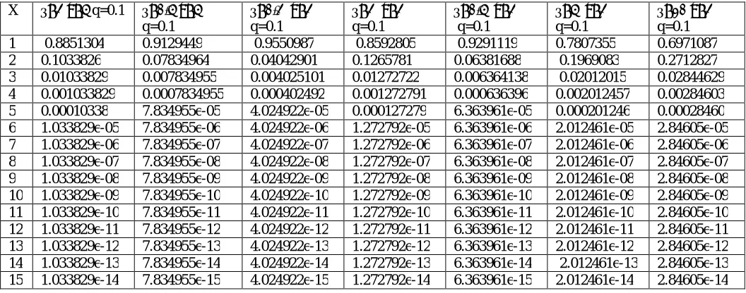
Table 1 The p.m.f. table of X~ HG (q,θ,k) , for different k and θ with q=0.1.

X θ=2 k=5 q=0.1 θ=0.5 k=5

q=0.1

θ=0.2 k=2 q=0.1

θ=2 k=2 q=0.1

θ=0.5 k=2 q=0.1

θ=5 k=2 q=0.1

θ=10 k=2 q=0.1

1 0.8851304 0.9129449 0.9550987 0.8592805 0.9291119 0.7807355 0.6971087

2 0.1033826 0.07834964 0.04042901 0.1265781 0.06381688 0.1969083 0.2712827

3 0.01033829 0.007834955 0.004025101 0.01272722 0.006364138 0.02012015 0.02844629

4 0.001033829 0.0007834955 0.000402492 0.001272791 0.000636396 0.002012457 0.00284603

5 0.00010338 7.834955e-05 4.024922e-05 0.000127279 6.363961e-05 0.000201246 0.00028460

6 1.033829e-05 7.834955e-06 4.024922e-06 1.272792e-05 6.363961e-06 2.012461e-05 2.84605e-05

7 1.033829e-06 7.834955e-07 4.024922e-07 1.272792e-06 6.363961e-07 2.012461e-06 2.84605e-06

8 1.033829e-07 7.834955e-08 4.024922e-08 1.272792e-07 6.363961e-08 2.012461e-07 2.84605e-07

9 1.033829e-08 7.834955e-09 4.024922e-09 1.272792e-08 6.363961e-09 2.012461e-08 2.84605e-08

10 1.033829e-09 7.834955e-10 4.024922e-10 1.272792e-09 6.363961e-10 2.012461e-09 2.84605e-09

11 1.033829e-10 7.834955e-11 4.024922e-11 1.272792e-10 6.363961e-11 2.012461e-10 2.84605e-10

12 1.033829e-11 7.834955e-12 4.024922e-12 1.272792e-11 6.363961e-12 2.012461e-11 2.84605e-11

13 1.033829e-12 7.834955e-13 4.024922e-13 1.272792e-12 6.363961e-13 2.012461e-12 2.84605e-12

14 1.033829e-13 7.834955e-14 4.024922e-14 1.272792e-13 6.363961e-14 2.012461e-13 2.84605e-13

(3)

ISSN(Online): 2319-8753

ISSN (Print): 2347-6710

I

nternational

J

ournal of

I

nnovative

R

esearch in

S

cience,

E

ngineering and

T

echnology

Table 2 The p.m.f. table of X~ HG (q,θ,k), for different k and θ.

X q=0.1θ=0.5

k=10 q=0.1θ=2 k=10 q=0.25θ=0.75 k=5 q=0.25θ=0.25 k=5 q=0.5θ=0.1 k=5 q=0.5θ=10 k=5

1 0.9066967 0.8928227 0.7639666 0.8105077 0.6827162 0.2458752

2 0.08397297 0.09645961 0.1770279 0.1421262 0.1595167 0.3585943

3 0.008397297 0.00964596 0.0442541 0.03552461 0.07889698 0.1974297

4 0.0008397297 0.00096459 0.01106353 0.00888115 0.03943526 0.09904511

5 8.397297e-05 9.645961e-05 0.002765881 0.00222028 0.01971742 0.04952774

6 8.397297e-06 9.645961e-06 0.0006914703 0.000555072 0.009858709 0.02476395

7 8.397297e-07 9.645961e-07 0.0001728676 0.000138768 0.004929354 0.01238198

8 8.397297e-08 9.645961e-08 4.32169e-05 3.4692e-05 0.002464677 0.006190989

9 8.397297e-09 9.645961e-09 1.080422e-05 8.673e-06 0.001232339 0.003095495

10 8.397297e-10 9.645961e-10 2.701056e-06 2.16825e-06 0.0006161693 0.001547747

11 8.397297e-11 9.645961e-11 6.75264e-07 5.420625e-07 0.0003080846 0.0007738736

12 8.397297e-12 9.645961e-12 1.68816e-07 1.355156e-07 0.0001540423 0.0003869368

13 8.397297e-13 9.645961e-13 4.2204e-08 3.387891e-08 7.702116e-05 0.0001934684

14 8.397297e-14 9.645961e-14 1.0551e-08 8.469726e-09 3.851058e-05 9.67342e-05

15 8.397297e-15 9.645961e-15 2.63775e-09 2.117432e-09 1.925529e-05 4.83671e-05

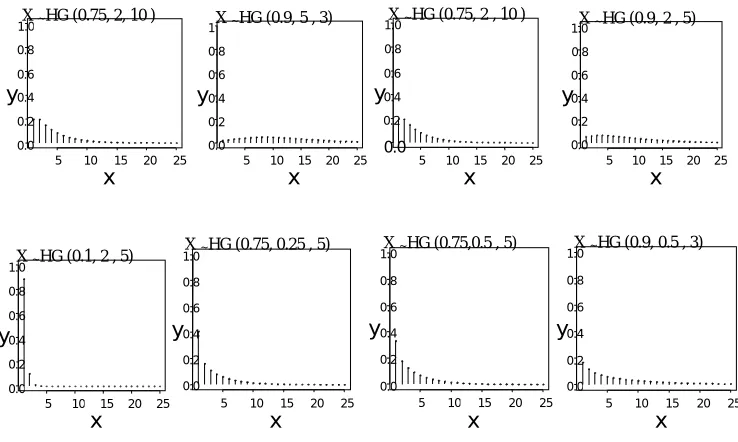
Figure 1 The p.m.f of X ~ HG (q,θ,k)

From (5), Figure 1 and Table 1 & Table 2 it is seen that,

Remark 3 For θ<1 p.m.f. of X~ HG (q,θ,k) decreasing with x.

5 10 15 20 25

0.0 0.2 0.4 0.6 0.8

1.0X ~ HG (0.9, 0.5 , 3)

x y

5 10 15 20 25

0.0 0.2 0.4 0.6 0.8

1.0X ~ HG (0.75,0.5 , 5)

x y

5 10 15 20 25

0.0 0.2 0.4 0.6 0.8

1.0X ~ HG (0.75, 0.25 , 5)

x y

5 10 15 20 25

0.0 0.2 0.4 0.6 0.8

1.0X ~ HG (0.1, 2 , 5)

x y

5 10 15 20 25

0.0 0.2 0.4 0.6 0.8

1.0X ~ HG (0.9, 2 , 5)

x y

5 10 15 20 25

0.0

0.2 0.4 0.6 0.8

1.0X ~ HG (0.75, 2 , 10 )

x y

5 10 15 20 25

0.0 0.2 0.4 0.6 0.8

1X ~ HG (0.9, 5 , 3)

x y

5 10 15 20 25

0.0 0.2 0.4 0.6 0.8

1.0X ~ HG (0.75, 2, 10 )

(4)

ISSN(Online): 2319-8753

ISSN (Print): 2347-6710

I

nternational

J

ournal of

I

nnovative

R

esearch in

S

cience,

E

ngineering and

T

echnology

III. 3 EXPECTATION, STANDARD DEVIATION AND ENTROPY OF HG DISTRIBUTION

We compute the expectation, standard deviation and Shannon’s entropy of the HG distribution with different ‘a, k’ and ‘θ’ (Table 3). For a discrete distribution, Shannon’s Entropy = -∑i p (xi) log p (xi), i = 1, 2…

Table 3 Expectation, standard deviation and Shannon’s entropy of X~ HG (q,θ,k) (With K=5)

k=5 q θ E(x) Sd(x) entropy k=5 q θ E(x) Sd(x) entropy

0.9 0.75 7.181742 6.24706 2.797387 0.5 2 2.145117 1.459823 1.476805

0.75 0.75 3.822205 3.363209 2.194411 0.1 2 1.127633 0.3737722 0.3980682

0.1 0.75 1.104899 0.3423532 0.346722 0.9 5 9.231612 6.478768 2.88427

0.9 0.5 6.761051 6.181877 2.741898 0.75 5 4.9415 3.514446 2.425729

0.75 0.5 3.61276 3.310981 2.120546 0.1 5 1.153302 0.4048062 0.4511009

0.1 0.5 1.096728 0.3299496 0.3271156 0.9 10 9.954691 6.57884 2.858474

0.75 0.2 3.186474 3.169406 1.934354 0.75 10 5.388573 3.538493 2.465914

0.1 0.2 1.080531 0.3032189 0.2861816 0.5 10 2.545866 1.524628 1.628365

0.9 2 8.238283 6.372622 2.875304 0.1 10 1.176096 0.4292081 0.4943981

0.75 2 4.376501 3.459642 2.338958 0.9 100 11.89503 7.275485 2.633785

A closer look with the entropy of X~HG (q,θ,k) with different q, θ and k (table 4 ).

Table 4 Entropy of X ~ HG (q,θ,k ) with different q, k & θ , (k=2).

k q θ=0.2 θ=0.5 θ =2 θ =5 θ =10 k q θ=0.2 θ=0.5 θ =2 θ =5 θ =10

2

0.9 2.549 2.988 3.450 3.631 3.718

5

0.9 2.891 3.118 3.349 3.435 3.475

0.75 1.608 1.997 2.447 2.629 2.717 0.75 1.939 2.126 2.347 2.435 2.476

0.5 0.892 1.171 1.575 1.758 1.848 0.5 1.159 1.289 1.476 1.576 1.628

0.1 0.199 0.281 0.457 0.606 0.726 0.1 0.286 0.327 0.398 0.451 0.494

Remark 4 When k increases, the entropy of X ~ HG (q,θ,k) increases with a fixed θ and q when (θ < 1) and decreases with a fixed θ and q when (θ>1).When θ increases the entropy of X ~ HG (q,θ,k) increases with a fixed q and k . Also when q increases the entropy of X ~ HG (q,θ,k) decreases with a fixed θ and k.

Remark 5For X~HG (q,θ,k) the E(X),the sd(X) and the entropy are greater than the E(X),the sd(X) and the entropy of X~MOG (q,θ) when θ < 1 and less than the E(X),the sd(X) and the entropy of X~MOG (q,θ) when θ >1.

Mean, median and mode of the HG distribution: Mean, median and mode of the HG distribution with different q

(5)

ISSN(Online): 2319-8753

ISSN (Print): 2347-6710

I

nternational

J

ournal of

I

nnovative

R

esearch in

S

cience,

E

ngineering and

T

echnology

Table 5 Mean, median and mode of the HG distribution with different qand θ (n = 100)

k q θ Mean Median Mode k q θ Mean Median Mode

5

0.1

0.1 1.07 1 1

5

0.75

0.1 2.92 1 1

0.25 1.084 1 1 0.25 3.3 2 1

0.5 1.09 1 1 0.5 3.63 2 1

2 1.081 1 1 2 4.401 3 2

4 1.092 1 1 4 4.829 4 2

10 1.176 1 1 10 5.423 4 3

0.5

0.1 1.632 1 1

0.9

0.1 6.849 3 1

0.25 1.759 1 1 0.25 7.98 5 1

0.5 1.871 1 1 0.5 8.945 6 1

2 2.145 2 1 2 11.12 8 4

4 2.307 2 1 4 12.3 10 6

10 2.545 2 2 10 13.45 11 8

From table 5 we observed that for X ~ HG (a,θ,k) the mean is always greater than median and mode, hence, Remark 6

For X ~ HG(a,θ,k) the mean is greater than median and mode, hence the HG distribution is always (irrespective of the

value of θ)positively skewed. This suggests that the HG distribution can be a good fit for positively skewed data.

Remark 7 For X ~ HG (q,θ,k) the mean, median and mode are less than or equal to the mean, median and mode of X ~

MOG(q, θ).( here k=1)

IV. 4 HAZARD FUNCTION

The hazard function, γH(x) = h(x)/H(x)= [(H̄(x-1,θ,k))/(H̄(x,θ,k))] –1

=[θ1/kqx-1/[1-(1-θ)q(x-1)k]1/k]]/[θ1/kqx /[1-(1-θ)qxk]1/k]]–1

= (1/q){ [1-(1-θ) qxk] / [1-(1-θ) q(x-1)k] }1/k –1. (6)

The hazard function for different p, k & θ is calculated and represented in Table 7. The graph of the Hazard function of

X, with different values for the parameters q, θ & k is shown in Figure 2.

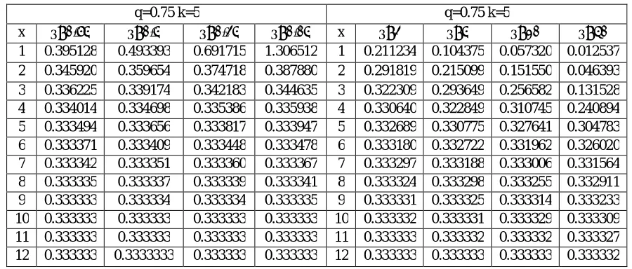
Table 7Hazard function γH(x) of X~HG (q,θ,k),q=0.75, θ < 1

q=0.75 k=5 q=0.75 k=5

x θ=0.75 θ=0.5 θ=0.25 θ=0.05 x θ=2 θ=5 θ=10 θ=50

1 0.395128 0.493393 0.691715 1.306512 1 0.211234 0.104375 0.057320 0.012537

2 0.345920 0.359654 0.374718 0.387880 2 0.291819 0.215099 0.151550 0.046393

3 0.336225 0.339174 0.342183 0.344635 3 0.322309 0.293649 0.256582 0.131528

4 0.334014 0.334698 0.335386 0.335938 4 0.330640 0.322849 0.310745 0.240894

5 0.333494 0.333656 0.333817 0.333947 5 0.332689 0.330775 0.327641 0.304783

6 0.333371 0.333409 0.333448 0.333478 6 0.333180 0.332722 0.331962 0.326020

7 0.333342 0.333351 0.333360 0.333367 7 0.333297 0.333188 0.333006 0.331564

8 0.333335 0.333337 0.333339 0.333341 8 0.333324 0.333298 0.333255 0.332911

9 0.333333 0.333334 0.333334 0.333335 9 0.333331 0.333325 0.333314 0.333233

10 0.333333 0.333333 0.333333 0.333333 10 0.333332 0.333331 0.333329 0.333309

11 0.333333 0.333333 0.333333 0.333333 11 0.333333 0.333332 0.333332 0.333327

(6)

ISSN(Online): 2319-8753

ISSN (Print): 2347-6710

I

nternational

J

ournal of

I

nnovative

R

esearch in

S

cience,

E

ngineering and

T

echnology

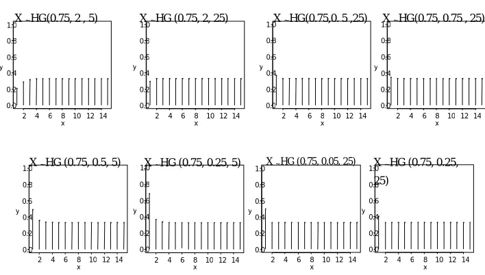
Figure 2 Hazard function of X~HG (q,θ,k)

It shows when θ > 1 the failure rate is non-decreasing and when θ <1 it is non-increasing. When x tends to 1, it is seen

that the hazard rate tends to a constant equal to(1/q) -1 = (p/q) for any θ > 0. From (6), Table 7 and Figure 2,

Remark 8 For X ~ HG (q, θ, k), when q is small the hazard rate tends to a constant equal to (1/q)-1= (p/q). i.e., γH(x) tends to p/q, irrespective of the value of θ.

Proof: For X ~ HG (q, θ,k), from (6), γH(x) = (1/q){ [1-(1-θ) qxk] / [1-(1-θ) q(x-1)k] }1/k – 1.

i.e., γH(x) = (1/q){ [1-(1-θ) qxk] / [1-(1-θ) qxk/qk] }1/k – 1 = (1/q){ [1-(1-θ) qxk] / [(qk -(1-θ) qxk)/qk] }1/k – 1.

i.e., as x tends to ∞, γH(x) tends to (1/q)-1 (here (1/q)-1 = p/q)

From the simulation results, it is seen that the rate of convergence is more rapidly when k is large.

Increasing /Decreasing failure rate (IFR/DFR): Let us define η(t) = 1 – [p(x=t+1) / p(x=t) ] & Δη(t) = η(t+1)-η(t). Kemp[4] showed, If Δη(t)>0, the distribution is with IFR, if Δη(t)<0 the distribution is with DFR and if Δη(t)=0 the distribution is with constant FR. Also Δη (t) = η (t+1) - η (t) = [P(x=t+1)/P(x=t)] –[P(x=t+2)/P(x=t+1)] >0, when

P(x=t+1)2 >P(x=t)P(x=t+2), then, the probabilities are log-concave and if [P(X=x+1)]2 <P(X=x)P(X=x+2) then

probabilities are log-convex. By definition 2.1 in (Sandhya and Prasanth [8])

Here, 1 – η (t)= h (t+1, θ, k)/ h (t,θ,k)

= θ1/k qt{[1/(1-(1-θ) qtk)1/k]-[q / (1-(1-θ)q(t+1)k)1/k]} / θ1/k qt-1{[1/ (1-(1-θ)q(t-1)k)1/k]- [q/(1-(1-θ) qtk)1/k ] }.

1 – η(t+1)= h(t+2,θ,k)/ h(t+1,θ,k)

= θ1/k qt+1{[1/ (1-(1-θ) q(t+1)k)1/k] - [q /(1-(1-θ) q(t+2)k)1/k ]}/θ1/k qt {[1/(1-(1-θ) qtk)1/k] - [q /(1-(1-θ) q(t+1)k)1/k]}.

Δη(t)= η(t+1)- η(t) ={1 –[h(t+2,θ,k)/ h(t+1,θ,k)]} – { 1 – [h(t+1,θ,k)/ h(t,θ,k)] }

That is when X~HG (q,θ,k), Δη(t) = { h(t+1,θ,k)/ h(t,θ,k) } – { h(t+2,θ,k)/ h(t+1,θ,k)}.

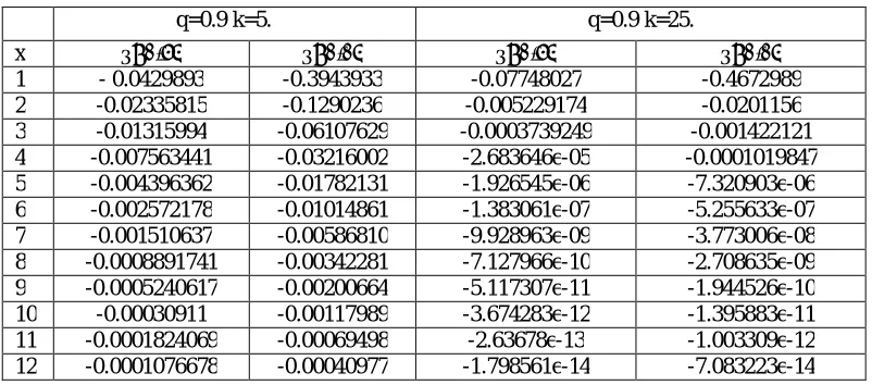
We can check it with different θ, k and q. then calculated Δη(t) in Table 8 and Table 9.

2 4 6 8 10 12 14 0.0

0.2 0.4 0.6 0.8

1.0X ~ HG (0.75, 0.25, 25)

x y

2 4 6 8 10 1214 0.0

0.2 0.4 0.6 0.8

1.0X ~ HG (0.75, 0.05, 25)

x y

2 4 6 8 10 12 14 0.0

0.2 0.4 0.6 0.8

1.0X ~ HG (0.75, 0.25, 5)

x y

2 4 6 8 10 12 14 0.0

0.2 0.4 0.6 0.8

1.0X ~ HG (0.75, 0.5, 5)

x y

2 4 6 8 10 12 14 0.0

0.2 0.4 0.6 0.8

1.0X ~ HG(0.75, 0.75 , 25)

x y

2 4 6 8 10 12 14 0.0

0.2 0.4 0.6 0.8

1.0X ~ HG(0.75,0. 5 ,25)

x y

2 4 6 8 10 12 14 0.0 0.2 0.4 0.6 0.8 1.0

X ~ HG (0.75, 2, 25)

x y

2 4 6 8 1012 14 0.0

0.2 0.4 0.6 0.8

1.0X ~ HG(0.75, 2 , 5)

(7)

ISSN(Online): 2319-8753

ISSN (Print): 2347-6710

I

nternational

J

ournal of

I

nnovative

R

esearch in

S

cience,

E

ngineering and

T

echnology

Table 8 Calculated Δη (t) of X →HG (q; θ; k), θ < 1

q=0.9 k=5. q=0.9 k=25.

x θ=0.75 θ=0.05 θ=0.75 θ=0.05

1 - 0.0429893 -0.3943933 -0.07748027 -0.4672989

2 -0.02335815 -0.1290236 -0.005229174 -0.0201156

3 -0.01315994 -0.06107629 -0.0003739249 -0.001422121

4 -0.007563441 -0.03216002 -2.683646e-05 -0.0001019847

5 -0.004396362 -0.01782131 -1.926545e-06 -7.320903e-06

6 -0.002572178 -0.01014861 -1.383061e-07 -5.255633e-07

7 -0.001510637 -0.00586810 -9.928963e-09 -3.773006e-08

8 -0.0008891741 -0.00342281 -7.127966e-10 -2.708635e-09

9 -0.0005240617 -0.00200664 -5.117307e-11 -1.944526e-10

10 -0.00030911 -0.00117989 -3.674283e-12 -1.395883e-11

11 -0.0001824069 -0.00069498 -2.63678e-13 -1.003309e-12

12 -0.0001076678 -0.00040977 -1.798561e-14 -7.083223e-14

Table 9 Calculated Δη(t) of X~HG (q,θ,k), θ > 1.

q=0.9 k=5. q=0.9 k=25.

x θ =5 θ=50 θ=5 θ=50

1 0.1012197 0.02357858 0.7631403 4.02686

2 0.1012504 0.0366706 0.07843443 0.6907295

3 0.08900311 0.05422491 0.005952379 0.06943551

4 0.06975785 0.07451798 0.000429225 0.005237675

5 0.04987859 0.09279671 3.08239e-05 0.000377487

6 0.03334167 0.1024701 2.212893e-06 2.710739e-05

7 0.02128242 0.0992576 1.588634e-07 1.946074e-06

8 0.01318267 0.08469318 1.140477e-08 1.397085e-07

9 0.008012775 0.06476242 8.187458e-10 1.002964e-08

10 0.004814235 0.04545278 5.877621e-11 7.20028e-10

11 0.002872283 0.02999003 4.2224e-12 5.168732e-11

12 0.00170649 0.01897888 3.009815e-13 3.714362e-12

So it’s clear that, for θ > 1, Δη(t) > 0 , and implies then the distribution is with IFR.Similarly when θ < 1, Δη(t) < 0 , the distribution is with DFR and when θ = 1 ,then Δη(t) = 0,the distribution is with constant FR . This constant FR is more often when X is large and when q is small the hazard rate tends to a constant equal to (1/q)-1= (p/q), (remark8) i.e. γH(x) tends to p/q. This is more rapidly when k is large.

Hence[P(X=x+1)] 2 <P(X=x) P(X=x+2) when θ<1. (7) i.e., probabilities are log-convex when θ < 1 and it is also seen that,

[P(X=x+1)] 2 > P(X=x) P(X=x+2) when θ > 1. (8) i.e., probabilities are log-concave when θ > 1

Remark 9 In discrete case, following Steutel [14], for distributions on non negative integers, log-convexity implies that they are compound geometric and hence they are infinitely divisible(i.d.) From Klebanov ,et.al [5], it is clear that

compound geometric distributions are Geometric infinitely divisible(GID)and that log-convexity implies that the

(8)

ISSN(Online): 2319-8753

ISSN (Print): 2347-6710

I

nternational

J

ournal of

I

nnovative

R

esearch in

S

cience,

E

ngineering and

T

echnology

Thus we have the following proposition

Proposition1 If a discrete random variable X ~HG(q,θ),x=1,2,3,…then, when 0< θ <1, the distribution is i) log-convex

ii)compound geometric ,iii)infinitely divisible (i.d.), iv)geometrically infinite divisible (GID), and with v) decreasing hazard rate (DHR).

Proof of (i) is clear from (7), and the remaining follows from the remark 9 and is similar to that of Theorem2.1, Sandhya and Prasanth [8].

New better than used/New worse than used (NBU/NWU):We know that, if the reliability function H̄t+x < H̄t H̄x then NBU and if H̄t+x > H̄t H̄x then NWU. (Adrinue W.Kemp [4]) explained the characteristics of discrete life-time

distributions)

Let X ~ H(q,ө,k) then, H̄x ,H̄t and H̄t+x are the s.fs of X=x,X=t and X=x+t respectively.

H̄t+x = θ1/k qt+x / [1-(1-θ) q(t+x)k]1/k, H̄x = θ1/k qx / [1-(1-θ) qxk]1/k, H̄t = θ1/k qt/ [1-(1-θ) qtk]1/k.

If θ > 1, then, H̄t+x < H̄t H̄xthen the distribution is NBU and if θ < 1, the distribution is NWU. Proof is similar to that of MOG distribution (Sandhya and Prasanth [8]).

Remark 10 For the Harris-Geometric distribution,

when θ > 1 , the distribution is log-convex  IFRIFRANBUNBUEDMRL &

when θ < 1, the distribution is log-concave  DFRDFRANWUNWUEIMRL. (By Remark 9)

Remark 11 Let γ F(x) and γ H(x,θ) are the Hazard rate of the geometric distribution and HG distribution respectively.

Then, i) Limit (x_α) γH(x,θ) = Limit( x_α )γF(x,θ) for anyθ≥ 0. ii)γF(x)/θ ≤γH(x,θ)≤γ F(x) ,θ ≥ 1. iii) γF(x)≤ γ H(x,θ)≤ γ F(x)/θ, 0

≤ θ ≤ 1. (Proof is so direct from 1.2 and 4.1).

V. 5. HG DISTRIBUTION AS THE DISTRIBUTION OF MINIMUM OF A SEQUENCE OF I.I.D. VARIABLES

The following theorem gives characterization of HG distribution as the minimum of a sequence of i.i.d. variables following geometric distribution.

Theorem 1 Let {Xi, i≥1} be a sequence of i.i.d. r.vs with common s.f F̄(x). Let N be a Harris r.v H1(θ, k; 1/k)

independent of {xi, i≥1}. such that P(N=n)= [(n/k)-1 C(n/k)-1] (θ)1/k (1-θ)((n-1)/k), n=1,1+k,1+2k,… k > 0 integer, 0 < θ < 1.

Let UN= min1≤i≤n(xi). Then {UN} is distributed as HarrisGeometric distribution if and only if {Xi} ~ geometric (p).

Proof: Let the s.f of UN is,

J̄(x) = P (UN > x)= ∑1∞ [F̄(x)] n P(X=x)= θ1/k F̄(x)/ [1-(1-θ)Fk̄(x)]1/k = θ1/k [(qx]/ [1-(1-θ)qxk]1/k = θ1/k/ [q-kx - (1-θ)] 1/k.

Which is the s.f of Harris- Geometric (q,θ,k).Retracing the steps we get the only if part.

VI. 6 AR (1) MODEL WITH HG DISTRIBUTION AS INNOVATION DISTRIBUTION

Consider k independent AR(1) sequences {Xi,n},i=1,2,…k, for all n>0 integer and some b>0

Λi Xi,n = b { Λi Xi,n-1} with probability p

= b { Λi Xi,n-1} Λ { Λi εi,n-1} with probability 1-p (9)

(9)

ISSN(Online): 2319-8753

ISSN (Print): 2347-6710

I

nternational

J

ournal of

I

nnovative

R

esearch in

S

cience,

E

ngineering and

T

echnology

Theorem 2 In an AR (1) process with structure (9),{Xi,n} is stationary Markovian with Harris Geometric (θ,a,k)

marginal if and only if {Єn} is distributed as Geometric distribution with parameter (q).

Proof H̄(t) ={θ F̄k

(bt)/[1-(1-θ) F̄k

(bt)}1/k. Then let F̄k

(bt) = qx, then

H̄(t) ={θ F̄k

(bt)/[1-(1-θ) F̄k

(bt)}1/k = [θ1/k qkx / [1 – (1 – θ) qkx]1/k = θ1/k / [q-kx – (1 – θ)] 1/k. So Xi, n is HG (q,θ,k). We

canshow the converse by retracing the steps.

VII. 7 MAXIMUM LIKELIHOOD ESTIMATES (M.L.E.) OF THE PARAMETERS OF HG (Q,Θ,K)

Let x1, x2…xn n independent random samples from HG (q,θ,k). Then from (5) we write the likelihood function

L of the distribution. By partial differentiation of L w.r.to q, θ & k and equate them to zero we formulate 3 non-linear equations. We calculated the m.l.e. of q, and k numerically (using Mathematica) as the solution of these three nonlinear equations.

VIII. 8 SOME APPLICATIONS OF HG DISTRIBUTION

Example 1.Sales of medicine - domcet / dompar/cetadom (domperidone(10mg) with paracetamol (500mg)) in each 50days (excluding Sundays /each 2months of one year ) from a medical shop in the Palghat city(in Kerala, India) are noted. Here X= number of customers (with or without medical prescription brought the medicine) for domcet/dompar

/cetadom medicine (domperidone with paracetamol).

Table 10 Observed frequencies in each 50 days (2 months)

x 1 2 3 4 5 6 7 8 9 10 11 12 13 14 15

month

May-June 25 8 8 1 2 0 4 1 0 1 0 0 0 0 0

July- August 21 7 6 4 2 1 2 3 1 0 2 0 0 0 0

September- October 26 9 4 3 3 0 1 4 0 1 0 0 0 0 0

November- December 24 9 3 2 5 2 1 1 2 0 0 1 0 0 0

January- February 26 9 3 3 2 2 1 1 2 0 0 0 0 0 0

March - April 24 10 1 5 2 2 2 0 1 0 1 1 0 1 0

We have analyzed all these data sets. For convenience we arbitrarily take 3 month groups and represent the results here. We observe the mean, median and mode of these data (Table 11).

Table 11 Mean median and mode of the data in May-June, Nov-Dec and March-April

Month mean median mode

May-June 2.48 1 1

Nov-Dec 2.8 2 1

(10)

ISSN(Online): 2319-8753

ISSN (Print): 2347-6710

I

nternational

J

ournal of

I

nnovative

R

esearch in

S

cience,

E

ngineering and

T

echnology

Since mean > mode and mean > median, the data exhibits positive skeweness and it is observed that the distribution is unimodal, hence HG distribution is supposed to give a better fit.

Table 12Goodness of fit of HG distribution using chi-square test with α = 0.05

May-June Nov-Dec March-April

m.l.e q^ 0.7501 0.7256 0.7697

m.l.e. θ^ 0.1888 0.2250 0.2151

m.l.ek^ 3(3.1106) 3(3.1695) 3(2.5632)

Observed χ2 4.294 2.0125 3.91

degrees freedom d.f. 4 4 4

p-value 0.3677 0.7335 0.4183

Result: From the p-values it is seen that here HG distribution is suitable here.

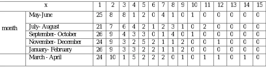
Example 2. Sales of medicine for kids – lanol / calpol / fepanil/ paracetamo/ flucold (with paracetamol (60ml-125mg)) within each 50days (excluding Sundays in each 2months of one year) from a medical shop in the Palghat city are noted .Here X= number of customers (with or without medical prescription brought the medicine) for lanol / calpol / fepanil/

paracetamol/ flucold (with paracetamol (60ml-125mg)).

x month

1 2 3 4 5 6 7 8 9 10 11 12 13 14 15 16 17 18 19

May-June 12 10 3 4 2 4 2 1 3 2 2 1 1 0 1 0 0 0 2

July- August 10 11 3 0 5 4 3 0 1 2 4 0 1 2 1 1 0 1 1

September- October 11 8 6 3 2 3 2 2 3 2 1 0 3 3 1 0 0 0 0

November- December 12 6 8 1 3 2 4 1 2 1 2 1 1 1 1 0 1 2 1

January- February 8 11 1 4 4 2 2 4 3 2 0 2 0 1 2 2 0 0 0

March - April 14 6 10 5 2 3 5 0 1 0 2 0 1 0 0 1 0 0 0

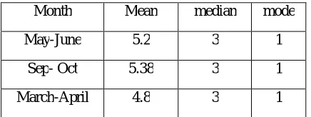
We analyzed all these data sets. For convenience we arbitrarily take 3 month groups and represent the results here. We observe the mean, median and mode of these data (Table 14).

Table 14 Mean median and mode of the data in May-June, September- October and March-April

Month Mean median mode

May-June 5.2 3 1

Sep- Oct 5.38 3 1

March-April 4.8 3 1

(11)

ISSN(Online): 2319-8753

ISSN (Print): 2347-6710

I

nternational

J

ournal of

I

nnovative

R

esearch in

S

cience,

E

ngineering and

T

echnology

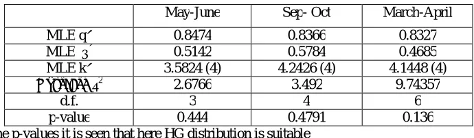
Table 15 Goodness of fit of HG distribution using chi-square test with α = 0.05

May-June Sep- Oct March-April

MLE q^ 0.8474 0.8366 0.8327

MLE θ^ 0.5142 0.5784 0.4685

MLE k^ 3.5824 (4) 4.2426 (4) 4.1448 (4)

Observed χ2 2.6766 3.492 9.74357

d.f. 3 4 6

p-value 0.444 0.4791 0.136

Result: From the p-values it is seen that here HG distribution is suitable

Example3 Sales of medicine for kids – lanol / calpol / fepanil/ paracetamol/ flucold (with paracetamol (60ml-125mg)) with any of the anti-biotic like Moxikind dispertab (amoxicillin trihydrate 125 mg) or any (with Azithromycin/Erythromycin/ Cefoperazonie/ Ampicllin/ Amoxicillin) within each 50days (excluding Sundays /each 2months of one year ) from a medical shop in the Palghat city are taken. Here X= number of customers (with or

without medical prescription brought the medicine) for lanol / calpol / fepanil/ paracetamol/ flucold (with paracetamol

(60ml-125mg)) with any of anti-biotic like Moxikind dispertab(amoxicillin trihydrate 125 mg) or (Azithromycin/ Erythromycin/Cefoperazone/Ampicillin/ Amoxicillin) within each 50 days

x month

1 2 3 4 5 6 7 8 9 10 11 12 13 14 15

May- June 13 19 6 7 5 0 0 0 0 0 0 0 0 0 0

July- August 11 15 13 5 3 1 1 1 0 0 0 0 0 0 0

September- October 12 16 13 4 2 1 1 0 1 0 0 0 0 0 0

November- December 9 18 11 6 3 0 0 0 0 0 1 0 2 0 0

January- February 8 12 10 13 3 1 0 0 2 0 0 1 0 0 0

March - April 11 11 16 7 1 0 2 2 0 0 0 0 0 0 0

We arbitrarily take 3 month groups and observe the mean, median and mode of these data (Table 17).

Table 17 Mean median and mode of the data in May-June, Sep - Oct and Nov-Dec

Month Mean median mode

May-June 2.44 2 2

Sep - Oct 2.62 2 2

Nov-Dec 3.08 2 2

Since mean > mode and mean > median, the data exhibits positive skeweness with m.l.e. of θ > 0 and it is observed that the distribution is unimodal, hence HG distribution is suppose to give a better fit.

Table 18 Goodness of fit of HG distribution with α = 0.05

Sample size = 50 MLE q^ MLE θ^ MLE k^ Observed χ2 d.f. p-value

May-June 0.4816 5.4108 2.1091 (2) 4.4928 4 0.3434

Sep - Oct 0.4936 5.0367 2.4050(2) 1.9735 4 0.7406

Nov-Dec 0.5211 5.2204 2.3670(2) 3.42 4 0.4901

(12)

ISSN(Online): 2319-8753

ISSN (Print): 2347-6710

I

nternational

J

ournal of

I

nnovative

R

esearch in

S

cience,

E

ngineering and

T

echnology

REFERENCES

[1] A.W. Marshall., and I.Olkin., “A New Method for Adding a Parameter to a Family of Distribution with Application to the Exponential and

Wiebull Families”, Biometrika,84.3pp 641-652, 1997. [2] Harris,T. E., “ Branching processes”, Annals of Mathematical Statistics, 19, 474–494, 1948.

[3] Johnson,N.L., Kotz,S and Kemp,A.W., “Univariate discrete distributions” , 2ndEdn., Wiley Newyork, 1992. [4] Kemp, A.W., “Classes of Discrete Lifetime Distributions”, Journal Communications in Statistics, Theory & Methods., 3069-3093, 2004

[5] Klebanov,L.B., Maniya,G.M., and Melamed,I.A., “A problem of zolotarev & analogs of i.d. and stable distributions in a scheme of summing a random number of random variables”, Theory& Prob.appl.,29,791-794, 1984. [6] Prasanth,C. B., and Sandhya, E., “A Generalized Discrete Uniform Distribution”, Journal of Statistics Applications & Probability, An

International Journal, Natural Sciences Publishing (NSP), 5, No. 1, 1-12, 2016 (accepted) [7] Sandhya, E., and Prasanth,C. B., “ Marshall-Olkin discrete uniform distribution”, Journal of Probability, Hindawi Publishing Corporation,

Volume 2014, 10 pages, 2013. [8] Sandhya, E., and Prasanth,C. B., “A Generalized Geometric distribution” , Proceedings of an International Conference on Frontiers of Statistics

and its Applications [ICONFROST-2012] & 32nd Annual Conference of Indian Society for Probability and Statistics [ISPS], Department of Statistics, Pondicherry University. December21–23, 2012. Bonfring Publication, 2012. [9] Sandhya, E., Sherly, S., and Raju, N., “Harris Family of Discrete Distributions”, Proceedings of National Seminar Conducted by Kerala Statistical

Association and The Dept.of statistics , University of Kerala, 2006a. [10] Sandhya, E., Sherly,S., Jose, K.K., and Raju, N., “Characterizations of the Extended Geometric ,Harris, Negative Binomial and Gamma

Distributions”, Stars int.Journal, 2006b. [11] Satheesh, S., Sandhya, E., and Sherly, S., “A Generalization of Stationary AR(1) Schemes”, Statistical Methods,8(2), 213-225, 2006.

[12] Satheesh, S., Sandhya, E., and Nair,N.U., “Stability of Random Sums”, Stoch. Modeling and Appl,5,17-26, 2002. [13] Satheesh,S., and Sandhya, E., “Infinite divisibility and max- infinite divisibility with random sample size”, Statist.Meth., 5, 126–139, 2003.

[14] Steutel,F.W., and van Harn,K., “ Infinite divisibility of distributions on the real line”, Marcel Dekker Inc., New York, 2004

.

BIOGRAPHY

Dr. Prasanth C B received his PhD degree in Statistics from Mahatma Gandhi University, Kerala, India under the supervision and guidance of Dr.E.Sandhya. His main research interests are: distribution theory, applied statistics, probability theory and study on urbanization. He has published research articles in reputed international and national journals

Dr.E.Sandhya took her Ph.D from the Department of Statistics,University of Kerala in 1992 under the supervision and guidance of Dr.R.N.Pillai. Her research interest includes

distribution theory,probability theory in general and infinite divisibility and geometric infinite divisibility and its extensions in particular. She has more than 35 published papers in various international and national publications. She is the reviewer for Mathematical Reviews of American Mathematical Society, USA .